lecture for complex variables

Lecture Notes for Complex Variables

James S. CookLiberty University

Department of Mathematics and Physics

Spring 2010

2

introduction and motivations for these notes

A complex variable is simply a variable whose possible values are allowed to reside in the complexnumbers. We’re using the classic text by Churchill and Brown:

”Complex Variables and Applications” by Churchill and Brown, 6-th Ed.

This text has been a staple of several generations of mathematicians at this time. I’ll try to followthe text somewhat closely. I plan to ask you to prove certain pivotal Lemmas as we develop thematerial together this semester. In previous courses you may have heard me advocate a certainpoint of view about complex numbers but I would ask you forget all that for a time. Our goal hereis to start from scratch and build complex numbers from the ”ground” up. The purpose of thesenotes is to complement Churchill’s text. I will try to add examples to expand on what is already inthe text. Also, I will try to give comments about connections to other fields of mathematics whereappropriate. Most of the theorems contained in these notes are likewise contained in Churchill andI will try to make a note when they are sufficiently famous. Other theorems are more the naturaloutgrowth of carefully chosen defintions and I probably will not source those theorems. I will tryto include some historical comments to help you understand how the theory of complex variableswas developed ( and is continuing to develop).We will use a fair amount of linear algebra in portions of this course, however if you have not hadmath 321 you should still be able to follow along.

Approximate Lecture List:

✓ history of complex numbers and competing defintions.

✓ algebraic properties of ℂ.

✓ polar form of complex numbers.

✓ complex logarithms and subtletites of multiply valued functions.

✓ topological properties of ℂ.

✓ continuous functions of a complex variable.

✓ complex differentiation and the Cauchy Riemann equations.

✓ the conjugate variable notation, homomorphic and antiholomorphic.

✓ Maximum modulus theorem.

✓ Cauchy-Goursat theorem.

✓ contour integration.

✓ Laurent series.

✓ geometric series techniques.

3

✓ theory of residues.

✓ integration techniques.

✓ proof of fundamental theorem of algebra.

✓ conformal mapping.

✓ Riemann surfaces.

Before we begin, I should warn you that I assume quite a few things from the reader. These notesare intended for someone who has already grappled with the problem of constructing proofs. Iassume you know the difference between ⇒ and ⇔. I assume the phrase ”iff” is known to you. Iassume you are ready and willing to do a proof by induction, strong or weak. I assume you knowwhat ℝ, ℚ, ℕ and ℤ denote. I assume you know what a subset of a set is. I assume you know howto prove two sets are equal. I assume you are familar with basic set operations such as union andintersection (although we don’t use those much). More importantly, I assume you have started toappreciate that mathematics is more than just calculations. Calculations without context, withouttheory, are doomed to failure. At a minimum theory and proper mathematics allows you to com-municate analytical concepts to other like-educated individuals.

Some of the most seemingly basic objects in mathematics are insidiously complex. We’ve beentaught they’re simple since our childhood, but as adults, mathematical adults, we find the actualdefinitions of such objects as ℝ is rather involved. I will not attempt to provide foundationalarguments to build real numbers from basic set theory. I believe it is possible, I think it’s well-thought-out mathematics, but we take the existence of the real numbers as an axiom for thesenotes. We assume that ℝ exists and that the real numbers possess all their usual properties. Infact, I assume ℝ, ℚ, ℕ and ℤ all exist complete with their standard properties. In short, I assumewe have numbers to work with. We leave the rigorization of real numbers to a different course.(truth is that complex numbers are relatively easy to construct once you have the starting point ofℝ.)Finally, please be warned these notes are a work in progress. I look forward to yourinput on how they can be improved, corrected and supplemented.

James Cook, January 19, 2010.

version 0.2

Contents

1 complex numbers 7

1.1 foundations of complex numbers . . . . . . . . . . . . . . . . . . . . . . . . . . . . . 7

1.2 complex conjugation . . . . . . . . . . . . . . . . . . . . . . . . . . . . . . . . . . . . 10

1.3 modulus and reality . . . . . . . . . . . . . . . . . . . . . . . . . . . . . . . . . . . . 12

1.4 polar form of complex numbers . . . . . . . . . . . . . . . . . . . . . . . . . . . . . . 15

1.5 complex exponential notation . . . . . . . . . . . . . . . . . . . . . . . . . . . . . . . 17

1.5.1 trigonmetric identities from the imaginary exponential . . . . . . . . . . . . . 21

1.6 complex roots of unity . . . . . . . . . . . . . . . . . . . . . . . . . . . . . . . . . . . 22

1.7 complex numbers and factoring . . . . . . . . . . . . . . . . . . . . . . . . . . . . . . 24

2 topology and mappings 27

2.1 open, closed and continuity in ℝn . . . . . . . . . . . . . . . . . . . . . . . . . . . . . 27

2.2 open, closed and continuity in ℂ . . . . . . . . . . . . . . . . . . . . . . . . . . . . . 30

2.2.1 complex functions are real mappings . . . . . . . . . . . . . . . . . . . . . . . 33

2.2.2 proofs on continuity of complex functions . . . . . . . . . . . . . . . . . . . . 34

2.3 connected sets, domains and regions . . . . . . . . . . . . . . . . . . . . . . . . . . . 38

2.4 Riemann sphere and the point at ∞ . . . . . . . . . . . . . . . . . . . . . . . . . . . 39

2.5 transformations and mappings . . . . . . . . . . . . . . . . . . . . . . . . . . . . . . 41

2.5.1 translations . . . . . . . . . . . . . . . . . . . . . . . . . . . . . . . . . . . . . 41

2.5.2 rotations . . . . . . . . . . . . . . . . . . . . . . . . . . . . . . . . . . . . . . 41

2.5.3 magnifications . . . . . . . . . . . . . . . . . . . . . . . . . . . . . . . . . . . 42

2.5.4 linear mappings . . . . . . . . . . . . . . . . . . . . . . . . . . . . . . . . . . . 42

2.5.5 the w = z2 mapping . . . . . . . . . . . . . . . . . . . . . . . . . . . . . . . . 43

2.5.6 the w = z1/2 mapping . . . . . . . . . . . . . . . . . . . . . . . . . . . . . . . 43

2.5.7 reciprocal mapping . . . . . . . . . . . . . . . . . . . . . . . . . . . . . . . . . 44

2.5.8 exponential mapping . . . . . . . . . . . . . . . . . . . . . . . . . . . . . . . . 44

2.6 branch cuts . . . . . . . . . . . . . . . . . . . . . . . . . . . . . . . . . . . . . . . . . 45

2.6.1 the principal root functions . . . . . . . . . . . . . . . . . . . . . . . . . . . . 45

2.6.2 logarithms . . . . . . . . . . . . . . . . . . . . . . . . . . . . . . . . . . . . . . 46

5

6 CONTENTS

3 complex differentiation 473.1 theory of differentiation for functions from ℝ2 to ℝ2 . . . . . . . . . . . . . . . . . . 483.2 complex linearity . . . . . . . . . . . . . . . . . . . . . . . . . . . . . . . . . . . . . . 493.3 complex differentiability and the Cauchy Riemann equations . . . . . . . . . . . . . 51

3.3.1 how to calculate df/dz via partial derivatives of components . . . . . . . . . . 543.3.2 Cauchy Riemann equations in polar coordinates . . . . . . . . . . . . . . . . 55

3.4 analytic functions . . . . . . . . . . . . . . . . . . . . . . . . . . . . . . . . . . . . . . 573.5 differentiation of complex valued functions of a real variable . . . . . . . . . . . . . . 613.6 analytic continuations . . . . . . . . . . . . . . . . . . . . . . . . . . . . . . . . . . . 643.7 trigonometric and hyperbolic functions . . . . . . . . . . . . . . . . . . . . . . . . . . 653.8 harmonic functions . . . . . . . . . . . . . . . . . . . . . . . . . . . . . . . . . . . . . 67

4 complex integration 714.1 integrals of a complex-valued function of a real variable . . . . . . . . . . . . . . . . 714.2 contour integrals . . . . . . . . . . . . . . . . . . . . . . . . . . . . . . . . . . . . . . 744.3 antiderivatives and analytic functions . . . . . . . . . . . . . . . . . . . . . . . . . . . 774.4 Cauchy Goursat and the deformation theorems . . . . . . . . . . . . . . . . . . . . . 774.5 Cauchy’s Integral Formula . . . . . . . . . . . . . . . . . . . . . . . . . . . . . . . . . 774.6 Lioville’s Theorem and the Fundmental Theorem of Algebra . . . . . . . . . . . . . . 77

5 Taylor and Laurent series 79

6 residue theory 81

7 residue theory 83

Chapter 1

complex numbers

1.1 foundations of complex numbers

Let’s begin with the definition of complex numbers due to Gauss. We assume that the real numbersexist with all their usual field axioms. Also, we assume that ℝn is the set of n-tuples of real numbers.For example, ℝ3 = {(x1, x2, x3) ∣ xi ∈ ℝ}.

Definition 1.1.1.

We define complex multiplication of points in ℝ2 according to the rule:

(x, y) ∗ (a, b) = (xa− yb, xb+ ya)

for all (x, y), (a, b) ∈ ℝ2. We define the real part of (x, y) by Re(x, y) = x and theimaginary part of (x, y) by Im(x, y) = y. We define complex addition and complexsubtraction by the usual operations on vectors in ℝ2

(x, y) + (a, b) = (x+ a, y + b) (x, y)− (a, b) = (x− a, y − b)

We say z ∈ ℝ2 is real iff Im(z) = 0. Likewise, z ∈ ℝ2 is said to be imaginary iff Re(z) = 0.

Notice that ∗ is a binary operation on ℝ2; in other words ∗ : ℝ2 × ℝ2 → ℝ2 is a function.Of course, there are many other binary operations you can imagine for the plane. What makesthis one so special is that it models all the desired algebraic traits of a complex number. Sincemany people are unwilling to cede the existence of mathematical objects merely on the basis ofalgebra this construction due to Gauss is nice. It gives us an answer to the question: ”what is acomplex number?” The answer is: ”you can view them as two dimensional vectors with a specialmultiplication”. There are many other answers but that is the one we mostly pursue in thesenotes1. At this point you should be saying to yourself, WHAT? How in the world is ℝ2 with ∗ thesame as the complex numbers ℂ we needed to solve quadratic equations? Let’s work it out.

1complex numbers can also be constructed from 2× 2 matrices or through field extension theory as you can studyin Math 422 at LU, there are likely other ways to construct complex numbers.

7

8 CHAPTER 1. COMPLEX NUMBERS

Proposition 1.1.2.

Let z ∈ ℝ2 then z ∗ (1, 0) = z and (1, 0) ∗ z = z therefore the vector (1, 0) is a multiplicativeidentity for complex multiplication.

Proof: suppose z = (x, y) ∈ ℝ2 then z ∗ (1, 0) = (x, y) ∗ (1, 0) = (x1 − y0, x0 + y1) = (x, y).Likewise, (1, 0) ∗ z = (1, 0) ∗ (x, y) = (1x− 0y, 1y + 0x) = (x, y) = z. □

Proposition 1.1.3.

The equation z ∗ z = (−1, 0) has solution (0, 1).

Proof: to say that (0, 1) solves the equation means that if we substitute it for z in the givenequation then the equation holds true. Note then

(0, 1) ∗ (0, 1) = (0(0)− 1(1), 0(1) + 1(0)) = (−1, 0). □

In the notation of later sections (−1, 0) = 1 and (0, 1) = i and we just proved that i2 = −1. Thisfunny vector multiplication gives us a way to build the imaginary number i.

Theorem 1.1.4. Complex numbers form a field.

Let v, w, z ∈ ℝ2 with z = (x, y) then

1. z + w = w + z; addition is commutative.

2. (v + w) + z = v + (w + z); addition is associative.

3. z + (0, 0) = z; additive identity.

4. z + (−x,−y) = (0, 0); additive inverse.

5. z ∗ w = w ∗ z; multiplication is commutative.

6. (v ∗ w) ∗ z = v ∗ (w ∗ z); multiplication is associative.

7. z ∗ (1, 0) = z; multiplicative identity.

8. for z ∕= 0 there exists z−1 such that z ∗ z−1 = (1, 0); additive inverse.

9. v ∗ (z + w) = v ∗ z + v ∗ w; distributive property.

Proof: each of these is proved by simply writing it out and using the definition of the ∗ multi-plication. Notice we already proved (7.). I’ll prove (8.) and (9.), Some of the others are in yourhomework.

1.1. FOUNDATIONS OF COMPLEX NUMBERS 9

Begin with (9.). Let v = (a, b), z = (x, y) and w = (r, t). Observe by defintion of ∗ and + on ℝ2,

v ∗ (z + w) = (a, b) ∗ [(x, y) + (r, t)]

= (a, b) ∗ (x+ r, y + t)

= (a(x+ r)− b(y + t), a(y + t) + b(x+ r))

= (ax+ ar − by − bt, ay + at+ bx+ br)

= (ax− by, ay + bx) + (ar − bt, at+ br)

= (a, b) ∗ (x, y) + (a, b) ∗ (r, t)

= v ∗ z + v + w.

Therefore (9.) is true for all v, w, z ∈ ℝ2. Notice in the calculation above I used the distributivefield axioms for ℝ several times.

To prove (8.) we first must search out the formula for z−1. Set it up as an algebra problem. We’regiven that z = (x, y) ∕= 0 hence either x ∕= 0 or y ∕= 0. We would like to find z−1 = (a, b) such that

(x, y) ∗ (a, b) = (1, 0) ⇒ (ax− by, xb+ ya) = (1, 0)

Thus by definition of vector equality,

ax− by = 1 and xb+ ya = 0

We’ll need to consider several cases.Case 1: x ∕= 0 but y = 0 then ax = 1 hence a = 1/x and so ya = 0 and it follows xb = 0 henceb = 0 and we deduce z−1 = (1/x, 0).Case 2: x = 0 but y ∕= 0 then −by = 1 hence b = −1/y and so xb = 0 and it follows ya = 0 hencea = 0 and we deduce z−1 = (0,−1/y).Case 3: x ∕= 0 and y ∕= 0 so we can divide by both x and y without fear,

xb+ ya = 0⇒ b = −ya/x

ax− by = 1 ⇒ ax+ y2a/x = 1 ⇒ a(x2 + y2) = x⇒ a =x

x2 + y2

Substitute that into b = −ya/x,

b =−yx

x

x2 + y2=

−yx2 + y2

Note that the formulas for cases 1 and 2 are also covered by 3 despite the fact that the derivationfor case 3 is nonsense in those cases, neat. To summarize:

z−1 =

(x

x2 + y2,−y

x2 + y2

).

The formula above solves z−1 ∗ z = (1, 0) for all z ∈ ℝ2 such that x2 + y2 ∕= 0. The proof of (8.)follows. □


Definition 1.1.5.

We define division of z by w for z, w ∈ ℝ2 where w ∕= 0 to be multiplication by the inverseof the reciprocal, z/w = z ∗ w−1.

Example 1.1.6. .

1.2 complex conjugation

Definition 1.2.1.

The complex conjugate of (x, y) ∈ ℝ2 is denoted (x, y) where we define (x, y) = (x,−y).

The complex conjugate of a vector is the reflection of the vector about the x-axis. Naturally if wedo two such reflections we’ll get back to where we started. I don’t suppose that all the propertieslisted in the theorem below are that easy to ”see”.

Theorem 1.2.2. Properties of conjugation.

Let z, w ∈ ℝ2,

1. z + w = z + w.

2. z ∗ w = z ∗ w.

3. z/w = z/w.

4. z = z

The properties above are easy to verify, I leave it to the reader or the test.

1.2. COMPLEX CONJUGATION 11


Let z ∈ ℝ2,

1. if z = (x, y) then z ∗ z = (x2 + y2, 0).

2. if z = (x, y) then (x, 0) = 1(2,0)(z + z)

3. if z = (x, y) then (y, 0) = 1(0,2)(z − z)

Proof: Begin with (1.),

z ∗ z = (x, y) ∗ (x,−y) = (x2 + y2,−xy + yx) = (x2 + y2, 0).

Now (2.),z + z = (x, y) + (x,−y) = (2x, 0) ⇒ z + z = (x, 0) ∗ (2, 0).

To see (3.) we subtract,

z − z = (x, y)− (x,−y) = (0, 2y) ⇒ z − z = (y, 0) ∗ (0, 2).

The theorem follows. □.

Remark 1.2.4.

I believe at this point we have proved enough properties of ℝ2 paired with ∗ to convince youthat we really can construct such a thing as ℂ. From this point onward I will revert to thestandard notation which assumes the things we have just proved in these notes so far. Inshort I will omit the ∗ and write (x, 0) = x and (0, y) = yi. The fundamental formulas are(1, 0) = 1 and (0, 1) = i. Thus we find the unit vectors in the Argand plane are precisely thenumber one and the imaginary number i. In view of this correspondence we find great logicin saying the vertical axes in the complex plane ℝ2 has unit vector i whereas the x-axes hasunit vector 1. We adopt the notation ℝ2 together with ∗ is ℂ.

Let me restate the theorem in less obtuse notation,


Let z ∈ ℂ,

1. if z = (x, y) then zz = x2 + y2.

2. if z = (x, y) then x = 12(z + z)

3. if z = (x, y) then y = 12i(z − z)

4. If z = Re(z) + iIm(z) then Re(z) = 12(z + z) and Im(z) = 1

2i(z − z).

We can also restate the field axioms with the ∗ omitted. Our custom will be the usual one throughtthe remainder of the course, we use juxtaposition to denote multiplication. At this point I havecovered what I am likely to cover from §1&2 of Churhill.


1.3 modulus and reality

The modulus of a complex number is the length of the corresponding vector in ℝ2.

Definition 1.3.1.

The modulus of z ∈ ℂ is denoted ∣z∣ where we define ∣z∣ =√zz.

Notice that item (1.) of Theorem 1.2.5 shows that zz is a non-negative quantity therefore thesquareroot will return a real, non-negative, quantity. We also can calculate the distance betweencomplex numbers via the modulus as follows:

Definition 1.3.2.

Let z, w ∈ ℂ. The distance between z and w is denoted d(z, w) and we define d(z, w) =∣z − w∣.

Let’s pause to contemplate the geometrical meaning of a few complex equations.

Example 1.3.3. .

Example 1.3.4. .

1.3. MODULUS AND REALITY 13

Notice that we cannot write inequalities for complex numbers with nonzero imaginary parts. Wehave no definition for z < w given arbitrary z, w ∈ ℂ. However, the modulus of a complex numberis a real number so we can write various inequalities. These will be important to limit argumentsin upcoming sections.

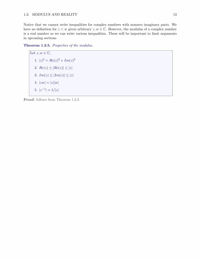
Theorem 1.3.5. Properties of the modulus.

Let z, w ∈ ℂ,

1. ∣z∣2 = Re(z)2 + Im(z)2

2. Re(z) ≤ ∣Re(z)∣ ≤ ∣z∣

3. Im(z) ≤ ∣Im(z)∣ ≤ ∣z∣

4. ∣zw∣ = ∣z∣∣w∣

5. ∣z−1∣ = 1/∣z∣

Proof: follows from Theorem 1.2.3.


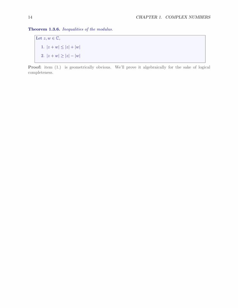
Theorem 1.3.6. Inequalities of the modulus.

Let z, w ∈ ℂ,

1. ∣z + w∣ ≤ ∣z∣+ ∣w∣

2. ∣z + w∣ ≥ ∣z∣ − ∣w∣

Proof: item (1.) is geometrically obvious. We’ll prove it algebraically for the sake of logicalcompleteness.

1.4. POLAR FORM OF COMPLEX NUMBERS 15

1.4 polar form of complex numbers

Given a point z = (x, y) = x+ iy in the complex plane we can find the polar coordinates in thesame way we did in calculus II or III. Recall that x = r cos(�) and y = r sin(�) so

x+ iy = r cos(�) + ir sin(�) = r(cos(�) + i sin(�))

However, we insist that r ≥ 0 in this course and the value for the angle requires some discussion.The trouble with angles is that one direction geometrically corresponds to infinitely many angles.This makes the angle a multiply-valued function (a contradiction in terms if you want to be critical!).To give a careful account of the ambiguity of choosing the angle we have to invent some notation tosummarize these concerns. This is the reason for ”arg” and ”Arg”. Be warned I am more carefulthan Churchill in my use of arg however I probably agree with his use of Arg.

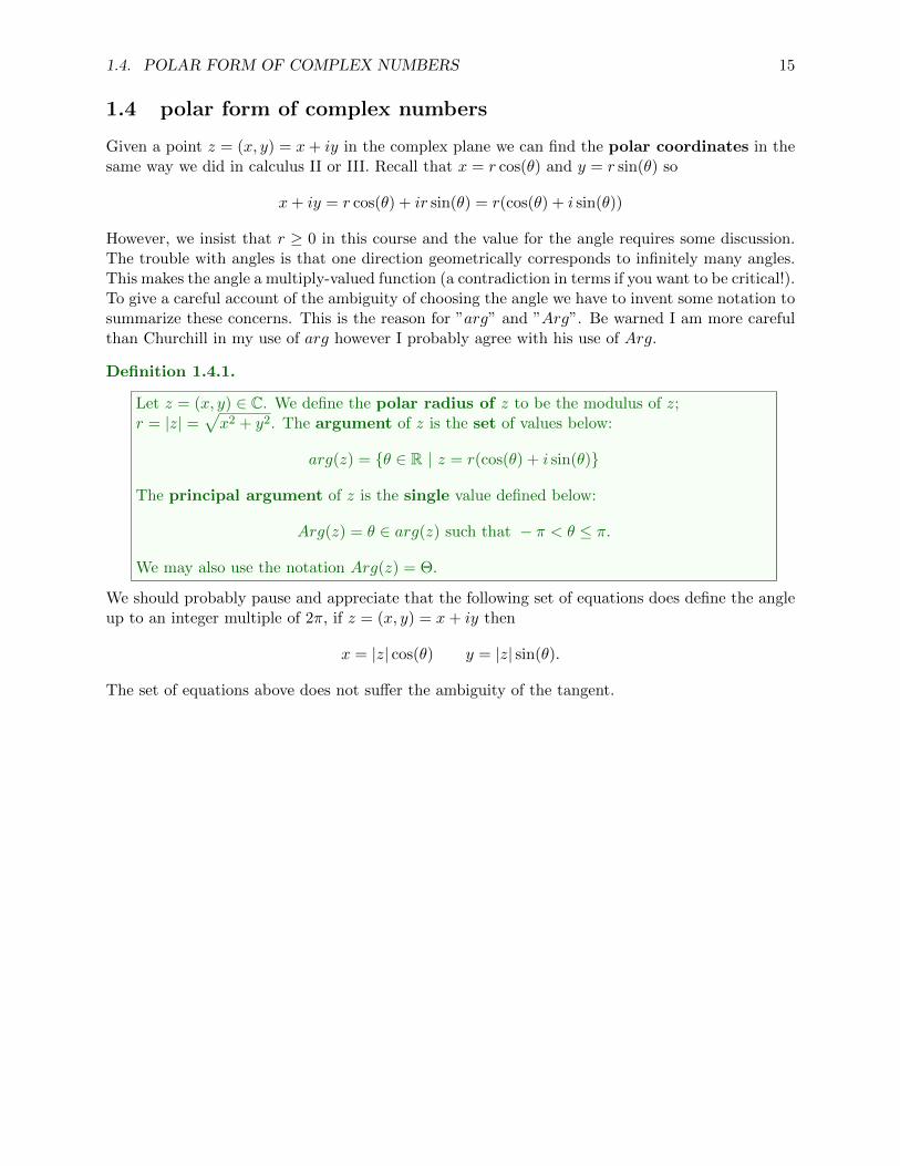
Definition 1.4.1.

Let z = (x, y) ∈ ℂ. We define the polar radius of z to be the modulus of z;r = ∣z∣ =

√x2 + y2. The argument of z is the set of values below:

arg(z) = {� ∈ ℝ ∣ z = r(cos(�) + i sin(�)}

The principal argument of z is the single value defined below:

Arg(z) = � ∈ arg(z) such that − � < � ≤ �.

We may also use the notation Arg(z) = Θ.

We should probably pause and appreciate that the following set of equations does define the angleup to an integer multiple of 2�, if z = (x, y) = x+ iy then

x = ∣z∣ cos(�) y = ∣z∣ sin(�).

The set of equations above does not suffer the ambiguity of the tangent.


Example 1.4.2. .

Example 1.4.3. .

1.5. COMPLEX EXPONENTIAL NOTATION 17

1.5 complex exponential notation

There are various approaches to this topic. I’ll get straight to the point here.

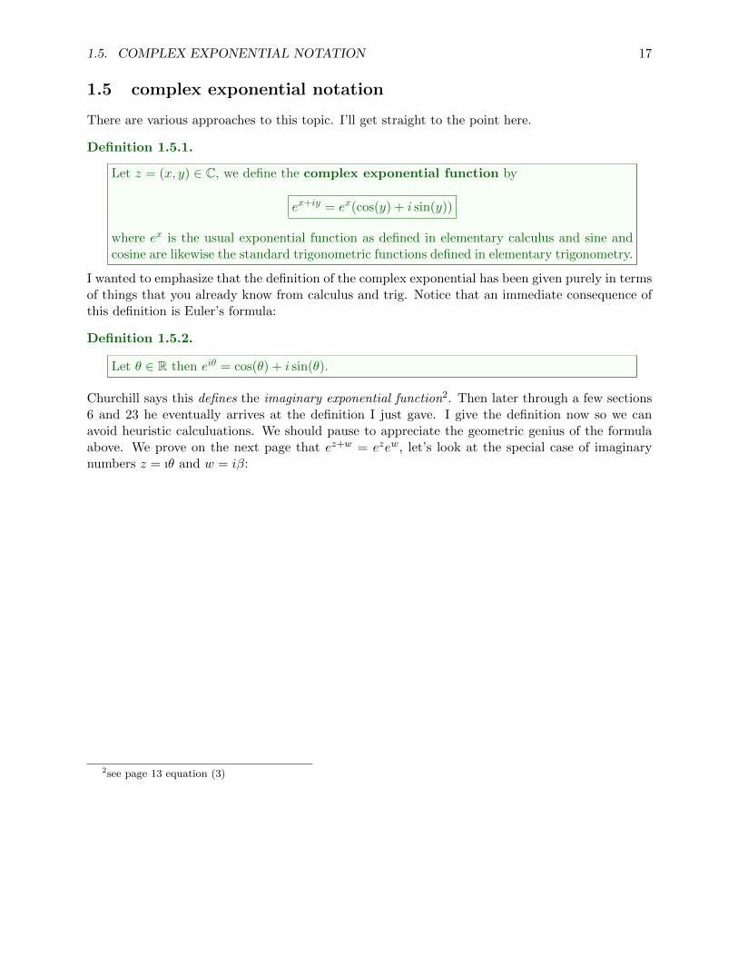
Definition 1.5.1.

Let z = (x, y) ∈ ℂ, we define the complex exponential function by

ex+iy = ex(cos(y) + i sin(y))

where ex is the usual exponential function as defined in elementary calculus and sine andcosine are likewise the standard trigonometric functions defined in elementary trigonometry.

I wanted to emphasize that the definition of the complex exponential has been given purely in termsof things that you already know from calculus and trig. Notice that an immediate consequence ofthis definition is Euler’s formula:

Definition 1.5.2.

Let � ∈ ℝ then ei� = cos(�) + i sin(�).

Churchill says this defines the imaginary exponential function2. Then later through a few sections6 and 23 he eventually arrives at the definition I just gave. I give the definition now so we canavoid heuristic calculuations. We should pause to appreciate the geometric genius of the formulaabove. We prove on the next page that ez+w = ezew, let’s look at the special case of imaginarynumbers z = ı� and w = i�:

2see page 13 equation (3)


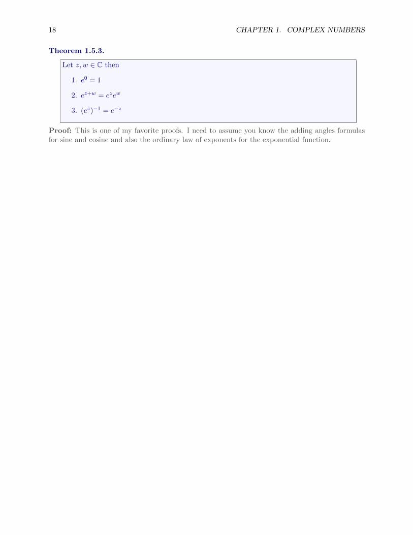
Theorem 1.5.3.

Let z, w ∈ ℂ then

1. e0 = 1

2. ez+w = ezew

3. (ez)−1 = e−z

Proof: This is one of my favorite proofs. I need to assume you know the adding angles formulasfor sine and cosine and also the ordinary law of exponents for the exponential function.


Theorem 1.5.4.

Let z ∈ ℂ and define (ez)n inductively by (ez)0 = 1 and (ez)n = (ez)n−1ez for all n ∈ ℕ.Likewise define (ez)−n = (e−z)n for all n ∈ ℕ.

1. (ez)n = enz for all n ∈ ℤ

2. if z = ∣z∣ei� then zn = ∣z∣n(cos(n�) + i sin(n�)) for n ∈ ℕ.

Proof: Notice that if we know (1.) holds for all z ∈ ℂ then we can use it to prove (2.). Observethat zn = (∣z∣ei�)n = (∣z∣ei�)n−1∣z∣ei� and you can prove by induction that zn = ∣z∣n(ei�)n. Apply(1.) to (ei�)n and we find zn = ∣z∣n(cos(n�) + i sin(n�)). I encourage the reader to supply theinduction argument omitted in the paragraph above. Incidentally, the formula

(cos(�) + i sin(�))n = cos(n�) + i sin(n�)

is called de Moivre’s formula. Let us prove (1.):


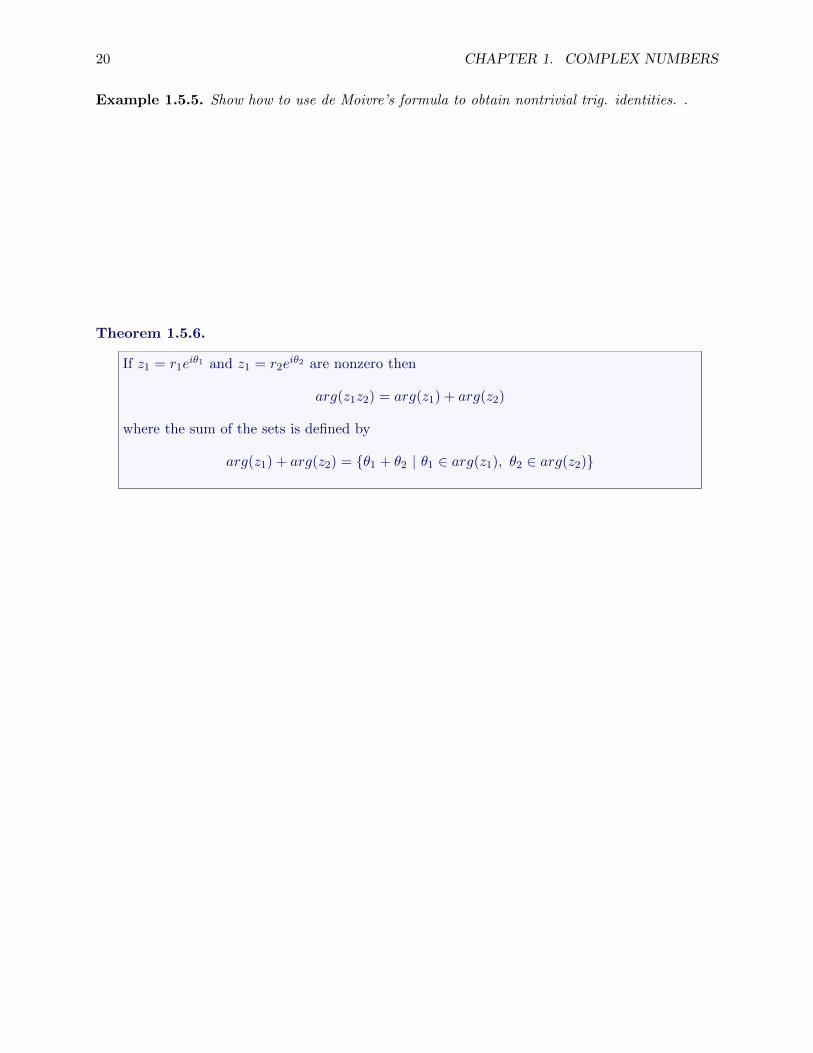
Example 1.5.5. Show how to use de Moivre’s formula to obtain nontrivial trig. identities. .

Theorem 1.5.6.

If z1 = r1ei�1 and z1 = r2e

i�2 are nonzero then

arg(z1z2) = arg(z1) + arg(z2)

where the sum of the sets is defined by

arg(z1) + arg(z2) = {�1 + �2 ∣ �1 ∈ arg(z1), �2 ∈ arg(z2)}


The practical meaning of Theorem 1.5.6 is that when we are faced with solving equations such asez = ew we must be careful to consider a multitude of possible cases. The complex exponentialfunction is far from one-one.

1.5.1 trigonmetric identities from the imaginary exponential

Now that we have a few of the basics settled let’s do a few interesting calculations. I probablydidn’t cover these in lecture.

Example 1.5.7. .

Example 1.5.8. .


1.6 complex roots of unity

In this section we examine the meaning of fractional exponent of a complex number. It turns out

that we cannot expect a single value. Instead we’ll learn that zmn is a set of values. The complex

roots of unity are used to generate the set of values. There is a neat connection between rotationsby � = 2�/n and ei� and ℤn.

Definition 1.6.1.

Let zo ∈ ℂ be nonzero. The n-th roots of zo is the set of values defined below:

z1/no = {z ∈ ℂ ∣ zn = zo}

Suppose that zo = roei�o and z = rei� then the requirement zn = zo yields

rnein� = roei�o

It follows that rn = ro and n�o = � + 2�k for some k ∈ ℤ. Therefore, if we denote the positiven-th root of the real number ro by n

√ro then r = n

√ro. Moreover, we may write the set of

roots as follows:

z1/no = { n

√roexp

[ i(�+2�k)n

]∣ k ∈ ℤ }

For example,11/2 = {exp(i2�k/2) ∣ k ∈ ℤ}

where I identified that � = 0 and ro = 1 since zo = 1ei0. Great, but what is this set 11/2? Noticethat

exp(i2�k/2) = cos(�k) + i sin(�k)

If k ∈ 2ℤ then k is an even integer and cos(�k) = 1. However, if k ∈ 2ℤ+1 then k is an odd integerand cos(�k) = −1. In all cases the sine term vanishes. We find,

11/2 = {1,−1}

To find the cube roots of 1 we’d examine the values of exp(i2�k/3) = cos(2�k/3) + i sin(2�k/3).We’d soon learn that k ∈ 3ℤ give exp(i2�k/3) = 1 whereas k ∈ 3ℤ + 1 give exp(i2�k/3) =

exp(2�/3) = cos(2�/3) + i sin(2�/3) = −12 + i

√3

2 and finally k ∈ 3ℤ + 2 give exp(i2�k/3) =

exp(4�/3) = −12 + i

√3

2 . We denote these by

11/3 = {1, !3, !23}

here !3 = exp(2�/3) = −12 + i

√3

2 is called the prinicpal cube root of unity. Naturally we cando this for any n ∈ ℕ and it is not hard to show that the n-th roots of unity are generated frompowers of !n = exp(2�/n). Indeed we could show that

11/n = {1, !n, !2n, . . . , !

n−1n }

1.6. COMPLEX ROOTS OF UNITY 23

The correspondence with ℤn = {0̄, 1̄, . . . , ¯n− 1} is provided by the mapping Φ(!kn) = k̄. You cancheck that Φ(zw) = Φ(z) + Φ(w). It is a homomorphism between the multiplicative group of unitsand the additive group ℤn.

Theorem 1.6.2.

If zo = roexp(i�o) then the n-th roots of zo are generated from the n-th roots of unity asfollows:

z1/no = {c, c!n, c!2

n, . . . , c!n−1n }

where c is a particular n-th root of zo; cn = zo. Notice that ∣c∣ = n

√ro and in the case

that 0 < zo ∈ ℝ we may choose c = n√ro where n

√ro denotes the positive n-th root of the

positive real number ro. In the formula above I am using our standard notation that !n isthe principal n-th root of unity which is given by the formula:

!n = exp(i2�/n).

Geometrically this theorem is very nice. It gives us a way to find the vectors which point to thevertices of a regular polygon with n-sides. Moreover, we can rotate the polygon by using a zo ∕= 1.

Example 1.6.3. .

Example 1.6.4. .

Example 1.6.5. .


1.7 complex numbers and factoring

In this section we examine a few examples of the factor theorem. This theorem states that everyzero of a complex polynomial corresponds to a factor. Don’t mind the definitions if you’re notinterested, just skip to the examples:

Definition 1.7.1.

A polynomial in x with coefficients in S is an expression

p(x) = c0 + c1x+ ⋅ ⋅ ⋅+ ckxk =

∞∑j=0

cjxj

where cj ∈ S for all j ∈ ℕ∪{0} and only finitely many of these coefficients are nonzero. Thedeg(p) = k if ck is the nonzero coefficient with the largest index k. We say that p(x) ∈ S(x).The set of polynomials in z with coefficients in ℂ is denoted ℂ (z). The set of polynomialsin z with coefficients in ℝ is denoted ℝ (z).

Remark 1.7.2.

In the definition above I am thinking of polynomials as abstract expressions. Notice we canadd, subtract and multiply polynomials provided we can perform the same operations in S.This makes S(x) a vector space over S if S is a field. However, if S is only a ring then theset of polynomials forms what is known as a module. Polynomials can be used to buildnumber systems through an algebraic construction called field extension. This materialis discussed in some depth in Math 422 at LU.

Obviously we are primarily interested in either ℂ (z) or ℝ (x) in most undergraduate mathematics.These are precisely the objects we learned to factor in highschool and so forth. Let me give aprecise definition of factoring. Since we can view ℝ (z) ⊂ ℂ (z) we will focus on ℂ (z) in remainderof this section.

Definition 1.7.3.

Suppose f(z), g(z), ℎ(z) ∈ ℂ (z). Suppose deg(ℎ), deg(g) ≥ 1. If f(z) = ℎ(z)g(z) then wesay that g(z) and ℎ(z) factor f(z). If f(z) has no factors then we say that f is irreducible.If deg(f) = 1 then we say f(z) is a linear factor.

Example 1.7.4. .

1.7. COMPLEX NUMBERS AND FACTORING 25

Example 1.7.5. .

Example 1.7.6. .

In the next chapter we discuss the concept of a complex function. Once we take that viewpoint wecan evaluate polynomials at complex numbers. It’s worth noticing that if (z− r) is a factor of f(z)then it follows f(c) = 0. The converse is also true; if f(r) = 0 for some r ∈ ℂ then f(z) = (z−r)g(z)where g(z) is some other polynomial (the proof of the converse is less obvious). In any event, ifyou believe me, then we have the following: (here I mean for cj , bj to denote complex constants)

c0 + c1z + ⋅ ⋅ ⋅+ cnzn = 0 for z = r ⇔ c0 + c1z + ⋅ ⋅ ⋅+ ckz

k = (z − r)(b0 + b1z + ⋅ ⋅ ⋅+ bmzm)

I sometimes refer to the calculation above as the fundmental theorem of algebra. We’ll probablyprove that theorem sometime this semester.

Chapter 2

topology and mappings

Mathematics is built with functions and sets for the most part. In this chapter we learn what acomplex function is and we examine a number of interesting features. Mappings are also studiedand contrasted with functions. Since a complex function is a real mapping we begin with a briefoverview of what is known about real mappings. Continuity of complex functions is then discussedin some depth. We then define connected sets, domains and regions. Next the extended complexplane as modeled by the Riemann sphere is introduced as a convenient device to capture limits at∞.We then examine a number of transformations and introduce the idea of the w-plane. Branch-cutsare defined to extract functions from multiply-valued functions. In particular, n-th root functionsis defined. The complex logarithm is defined as a local inverse to the complex exponential. Wediscover many of the standad examples in this chapter. Notable exceptions are sine, cosine andhyperbolic sine or cosine etc... We focus on algebraic functions and the complex exponential.

2.1 open, closed and continuity in ℝn

In this section we describe the metric topology for ℝn. The topology is built via the Euclideannorm which is denoted by ∣∣⋅∣∣ : ℝn×ℝn → ℝ where ∣∣x∣∣ =

√x ⋅ x and x⋅x denotes the dot-product

where x ⋅ y = x1y1 + ⋅ ⋅ ⋅xnyn for all x, y ∈ ℝn. Once we’re done with this section I will recapitulatemany of the definitions given in this section in the special case of ℝ2 = ℂ where we have the familarformula ∣z∣ =

√zz and this is in fact the same idea of length; ∣z∣ = ∣∣z∣∣. These notes are borrowed

from my advanced calculus notes which in turn mirror the excellent text by Edwards on the subject.

In the study of functions of one real variable we often need to refer to open or closed intervals. Thedefinition that follows generalizes those concepts to n-dimensions.

Definition 2.1.1.

An open ball of radius � centered at a ∈ ℝn is the subset all points in ℝn which are lessthan � units from a, we denote this open ball by B�(a) = {x ∈ ℝn ∣ ∣∣x− a∣∣ < �}.The closed ball of radius � centered at a ∈ ℝn is likewise defined byB�(a) = {x ∈ ℝn ∣ ∣∣x− a∣∣ ≤ �}.

27

28 CHAPTER 2. TOPOLOGY AND MAPPINGS

Notice that in the n = 1 case we observe an open ball is an open interval: let a ∈ ℝ,

B�(a) = {x ∈ ℝ ∣ ∣∣x− a∣∣ < �} = {x ∈ ℝ ∣ ∣x− a∣ < �} = (a− �, a+ �)

In the n = 2 case we observe that an open ball is an open disk: let (a, b) ∈ ℝ2,

B�((a, b)) ={

(x, y) ∈ ℝ2 ∣ ∣∣ (x, y)− (a, b) ∣∣ < �}

={

(x, y) ∈ ℝ2 ∣√

(x− a)2 + (y − b)2 < �}

For n = 3 an open-ball is a sphere without the outer shell. In contrast, a closed ball in n = 3 is asolid sphere which includes the outer shell of the sphere.

Example 2.1.2. . .

Definition 2.1.3.

Let D ⊆ ℝn. We say y ∈ D is an interior point of D iff there exists some open ballcentered at y which is completely contained in D. We say y ∈ ℝn is a limit point of D iffevery open ball centered at y contains points in D − {y}. We say y ∈ ℝn is a boundarypoint of D iff every open ball centered at y contains points not in D and other points whichare in D − {y}. We say y ∈ D is an isolated point or exterior point of D if there existopen balls about y which do not contain other points in D. The set of all interior pointsof D is called the interior of D. Likewise the set of all boundary points for D is denoted∂D. The closure of D is defined to be D = D ∪ {y ∈ ℝn ∣ y a limit point}

If you’re like me the paragraph above doesn’t help much until I see the picture below. All the termsare aptly named. The term ”limit point” is given because those points are the ones for which it isnatural to define a limit.

Example 2.1.4. . .

Definition 2.1.5.

Let A ⊆ ℝn is an open set iff for each x ∈ A there exists � > 0 such that x ∈ B�(x) andB�(x) ⊂ A. Let B ⊆ ℝn is an closed set iff it contains all of its boundary points.

In calculus I the limit of a function is defined in terms of deleted open intervals centered about thelimit point. The limit of a mapping is likewise defined via deleted open balls:

2.1. OPEN, CLOSED AND CONTINUITY IN ℝN 29

Definition 2.1.6.

Let f : U ⊆ ℝn → V ⊆ ℝm be a mapping. We say that f has limit b ∈ ℝm at limit point aof U iff for each � > 0 there exists a � > 0 such that x ∈ ℝn with 0 < ∣∣x− a∣∣ < � implies∣∣f(x)− b∣∣ < �. In such a case we can denote the above by stating that limx→a f(x) = b.

Definition 2.1.7.

Let f : U ⊆ ℝn → V ⊆ ℝm be a mapping. If a ∈ U is a limit point of f then we say that fis continuous at a iff

limx→a

f(x) = f(a)

If a ∈ U is an isolated point then we also say that f is continuous at a. The mapping f iscontinuous on S iff it is continuous at each point in S. The mapping f is continuousiff it is continuous on its domain.

Notice that in the m = n = 1 case we recover the definition of continuous functions from calc.I. It turns out that most of the theorems for continuous functions transfer over to appropriatelygeneralized theorems on mappings. The proofs can be found in Edwards.

Proposition 2.1.8.

Suppose that f : U ⊆ ℝn → V ⊆ ℝm is a mapping with component functions f1, f2, . . . , fm.Let a ∈ U be a limit point of f then f is continous at a iff fj is continuous at a forj = 1, 2, . . . ,m. Moreover, f is continuous on S iff all the component functions of f arecontinuous on S. Finally, a mapping f is continous iff all of its component functions arecontinuous. .

Proposition 2.1.9.

Let f and g be mappings such that f ∘ g is well-defined. The composite function f ∘ g iscontinuous for points a ∈ dom(f ∘ g) such that the following two conditions hold:

1. g is continuous at a

2. f is continuous at g(a).

The proof of the proposition is in Edwards, it’s his Theorem 7.2. I’ll prove this theorem in aparticular context in this chapter.

Proposition 2.1.10.

Assume f, g : U ⊆ ℝn → V ⊆ ℝ are continuous functions at a ∈ U and suppose c ∈ ℝ.

1. f + g is continuous at a.

2. fg is continuous at a

3. cf is continuous at a.

Moreover, if f, g are continuous then f + g, fg and cf are continuous.


2.2 open, closed and continuity in ℂ

The definitions of the preceding section remain unaltered except that we specialize to two dimen-sions and use appropriate complex notation in this section. Trade the word ”ball” for ”disk” and”norm” for ”modulus”. Just to remind you the connection between the modulus and norm is simplythe following:

∣z∣ =√zz =

√x2 + y2 = ∣∣(x, y)∣∣.

Definition 2.2.1.

An open disk of radius � centered at zo ∈ ℂ is the subset all complex numbers which areless than an � distance from zo, we denote this open ball by

D�(zo) = {z ∈ ℂ ∣ ∣z − zo∣ < �}.

The deleted-disk with radius � centered at zo is likewise defined

Do� (zo) = {z ∈ ℂ ∣ 0 < ∣z − zo∣ < �}.

The closed disk of radius � centered at zo ∈ ℂ is defined by

D�(zo) = {z ∈ ℂ ∣ ∣z − zo∣ ≤ �}

.

The following definition is nearly unchanged from the preceding section.

Definition 2.2.2.

Let S ⊆ ℂ. We say y ∈ S is an interior point of S iff there exists some open disk centeredat y which is completely contained in S. We say y ∈ ℂ is a limit point of S iff every opendisk centered at y contains points in S − {y}. We say y ∈ ℂ is a boundary point of Siff every open disk centered at y contains points not in S and other points which are inS − {y}. We say y ∈ S is an isolated point or exterior point of S if there exist opendisks about y which do not contain other points in S. The set of all interior points of S iscalled the interior of S. Likewise the set of all boundary points for S is denoted ∂S. Theclosure of S is defined to be S = S ∪ {y ∈ ℂ ∣ y a limit point of S}

Perhaps the following picture helps clarify these definitions: .

2.2. OPEN, CLOSED AND CONTINUITY IN ℂ 31

Definition 2.2.3.

Let S ⊆ ℂ is an open set iff for each z ∈ S there exists � > 0 such that D�(z) ⊂ S. IfB ⊆ ℂ then B is a closed set iff it contains all of its boundary points. In other words, aclosed set S has ∂S ⊂ S.

A complex function is simply a function whose domain and codomain are subsets of ℂ.

Definition 2.2.4.

Let f : U ⊆ ℂ → V ⊆ ℂ be a complex function. We say that f has limit wo ∈ ℂat limit point zo of U iff for each � > 0 there exists a � > 0 such that z ∈ ℂ with0 < ∣z − zo∣ < � implies ∣f(z)−wo∣ < �. In such a case we can denote the above by statingthat limz→zo f(z) = wo. In other words, we say limz→zo f(z) = wo iff for each � > 0 thereexists a � > 0 such that f(Do

�(zo)) ⊂ D�(wo).

Example 2.2.5. . .

We should also note that zo need not be inside the domain of f in the limit. In the special casethat f(zo) is defined and f(zo) = wo we say the complex function is continuous at zo.

Definition 2.2.6.

Let f : U ⊆ ℂ→ V ⊆ ℂ be a complex function. If zo ∈ U is a limit point of f then we saythat f is continuous at a iff

limz→zo

f(z) = f(zo)

If zo ∈ U is an isolated point then we also say that f is continuous at zo. The function f iscontinuous on S iff it is continuous at each point in S. The function f is continuousiff it is continuous on its domain.

Example 2.2.7. . .


We postpone the proof of the proposition below until the end of this section. In short, most of thelimit theorems for real-valued functions generalize naturally to the context of ℂ.

Proposition 2.2.8.

Assume f, g : U ⊆ ℂ→ V ⊆ ℂ are functions with limit point zo ∈ U where the limits of fand g exist at zo.

1. limz→zo(f(z) + g(z)

)= limz→zo f(z) + limz→zo g(z).

2. limz→zo(f(z)g(z)

)=

(limz→zo f(z)

)(limz→zo g(z)

).

3. if c ∈ ℂ then limz→zo(cf(z)

)= c

(limz→zo f(z)

).

4. if limz→zo g(z) ∕= 0 then limz→zo[ f(z)g(z)

]= limz→zo f(z)

limz→zo g(z).

5. if ℎ : dom(ℎ)→ ℂ is continuous at limz→zo f(z) then

limz→zo

ℎ(f(z)) = f( limz→zo

f(z)).

An immediate consequence of the theorem above is that the sum, product, quotient and composite ofcontinuous complex functions is again continuous. Moreover, induction can be used to extend theseresults to power functions of z and arbitrary finite sums. It then follows that complex polynomialsare continuous on ℂ. A complex rational function is defined pointwise as the quotient of twocomplex polynomials. Rational functions in ℂ are continuous for points where the denominatorpolynomial is nonzero.

Example 2.2.9. . .

Example 2.2.10. .


2.2.1 complex functions are real mappings

If the complex function is as simple as the last example then the direct computation of limits viathe modulus is not too difficult. However, in general it is nice to be able to apply the calculus ofmany real variables. Notice that f : dom(f) ⊆ ℂ→ ℂ then we can split each output of the functioninto its real and imaginary part. We define:

u(z) = Re(f(z)) v(z) = Im(f(z))

Therefore, since Re(f(z)), Im(f(z)) ∈ ℝ for all z ∈ dom(f) there exist real-valued functions u, v :dom(f)→ ℝ such that

f(z) = u(z) + iv(z).

Moreover, since or convention is to write z = x+ iy = (x, y) we can view a complex function as amapping from dom(f) ⊆ ℝ2 to ℝ2 where

f(x+ iy) = u(x, y) + iv(x, y)

This is a standard notation in most texts.

Example 2.2.11. . .

Example 2.2.12. . .

Example 2.2.13. . .

Example 2.2.14. . .


2.2.2 proofs on continuity of complex functions

To begin note that if f = u + iv is a complex function then we may as well identify f = (u, v) asa mapping from ℝ2 to ℝ2 with component functions f1 = u and f2 = v. Therefore, by Proposition2.1.8 we find:

Proposition 2.2.15.

If f : D ⊆ ℂ → ℂ is a complex function with f(x + iy) = u(x, y) + iv(x, y) for all(x, y) ∈ D then f is continuous at zo ∈ D as a complex function iff u and v are continuousat zo = (xo, yo) ∈ D as real functions from dom(f) ⊆ ℝ2 to ℝ. Moreover, a complexfunction is continuous iff its component functions are continuous real functions.

Proof: it is interesting that the proof in Edwards is similar, just it uses norms instead of modulus.In any event, since you may not have had advanced calculus it’s probably best for me to includethis proof here:


In view of Proposition 2.2.15 we can easily deduce that Examples 2.2.11 - 2.2.14 give complexfunctions that are mostly continuous. I assume you recall the definition of continuous functionsof two variables from calculus III, remember the function g(x, y) is continuous iff the limit of thefunction g(r⃗(t)) → g(p) as t → 0 for all curves t → r⃗(t) with r⃗(0) = p. Typically we only employthis definition directly for the purpose of finding a contradiction. If you can show the limit isdifferent along two different paths then the limit does not exist. Of course, to be rigorous oneshould consult the �− � definition of continuity offered in the preceding section.

Example 2.2.16. . .

The proof of the following proposition is identical to the proof given in Edwards for the generalcase. I leave the proof as an exercise for the reader.

Proposition 2.2.17.

Let f and g be complex functions such that f ∘ g is well-defined. The composite functionf ∘ g is continuous for points a ∈ dom(f ∘ g) such that the following two conditions hold:

1. g is continuous at a

2. f is continuous at g(a).

The proof of part (1.) the following theorem is identical to the proof given in Edwards for thegeneral case. I will show that (2.) and (3.) also follow from the corresponding proposition for sumsand products of real functions. Then I give a second proof which does not borrow from the theoryof real mappings.

Proposition 2.2.18.

Assume f, g : U ⊆ ℝn → V ⊆ ℝ are continuous functions at zo ∈ U and suppose c ∈ ℝ.

1. f + g is continuous at zo.

2. fg is continuous at zo

3. cf is continuous at zo.

Moreover, if f, g are continuous then f + g, fg and cf are continuous.


Proof: We begin with the proof of (2.). Suppose f = u + iv and g = a + ib are continuous at zoand note, omitting the z-dependence,

fg = (u+ iv)(a+ ib) = ua− vb+ i(ub+ va).

In terms of real notation we have fg = (ua− vb, ub+ va). But, we know u, v, a, b are continuous atzo because they are the component functions of continuous functions f, g. Moreover, we find fg iscontinuous at zo since it has component functions (fg)1 = ua− vb and (fg)2 = ub+ va which arethe sum or difference of products of continuous functions at zo.

To prove (3.) just take the constant function g(z) = c. I leave the proof that the constant functionis continuous as an exercise for the reader. □

Hopefully you’ve noticed that the heart of the proofs given above were stolen from the correspond-ing theorems of real mappings. I did this purposefully because I want to draw a clear distinctionbetween these results on continuity and the later results we’ll find for complex differentiability. Theproof that follows is self-contained.

Proof: Suppose limz→zo f(z) = fo and limz→zo g(z) = go. Let � > 0. Since the limit of f at zoexists we can find �f > 0 such that 0 < ∣z − zo∣ < �f implies ∣f(z) − fo∣ < �/2. Likewise, as thelimit of g at zo exists we can find �g > 0 such that 0 < ∣z − zo∣ < �g implies ∣g(z) − go∣ < �/2.Suppose that � = min(�f , �g) and assume that z ∈ Do

�(zo). It follows that

∣(f + g)(z)− (fo + go)∣ = ∣f(z) + g(z)− fo − go∣ ≤ ∣f(z)− fo∣+ ∣g(z)− go∣ < �/2 + �/2 = �.

Thus 0 < ∣z − zo∣ < � implies ∣(f + g)(z)− (fo + go)∣ < �. Therefore,

limz→zo

(f(z) + g(z)) = limz→zo

f(z) + limz→zo

g(z)

Part (1.) of the proposition follows immediately.

Preparing for the proof of (2): We need to study ∣f(z)g(z)− fogo∣. Consider that

∣f(z)g(z)− fogo∣ = ∣f(z)g(z)− f(z)go + f(z)go − fogo∣ =∣∣f(z)

(g(z)− go

)+(f(z)− fo

)go∣∣

Then we can use properties of the modulus to find:

∣f(z)g(z)− fogo∣ ≤ ∣f(z)∣∣g(z)− go∣+ ∣go∣∣f(z)− fo∣

Note that we can choose a � > 0 such that if z ∈ Do�(zo) then both ∣g(z)− go∣ and ∣f(z)− fo∣ are

as small as we’d like. Furthermore, if ∣f(z)− fo∣ < � then ∣f(z)∣ < ∣fo∣+ �. Consider then that if∣f(z)− fo∣ < � and ∣g(z)− go∣ < � it follows that

∣f(z)g(z)− fogo∣ < (∣fo∣+ �)∣� + ∣go∣� = �2 + �(∣fo∣+ ∣go∣

)


Our goal is to find a � such that z ∈ Do�(zo) implies ∣f(z)g(z)−fogo∣ < �. In view of our calculations

up to this point we see that this can be accomplished if we could choose � such that

�2 + �(∣fo∣+ ∣go∣

)= �.

Apply the quadatric equation to find

� =−∣fo∣ − ∣go∣ ±

√(∣fo∣+ ∣go∣)2 + 4�

2

Note that it is clear that the (+) solution does yield � > 0.

Proof: Let � > 0. Define

� =−∣fo∣ − ∣go∣+

√(∣fo∣+ ∣go∣)2 + 4�

2.

Since the limits of f and g exist it follows that we choose � > 0 such that z ∈ Do�(zo) implies both

∣g(z) − go∣ < � and ∣f(z) − fo∣ < �. The following calculations were justified in the paragraphpreceding the proof:

∣f(z)g(z)− fogo∣ < �2 + �(∣fo∣+ ∣go∣

)= �.

Therefore,

limz→zo

f(z)g(z) =

(limz→zo

f(z)

)(limz→zo

g(z)

)Part (2.) of the proposition follows immediately. □.


2.3 connected sets, domains and regions

To avoid certain pathological cases we often insist that the set considered is a domain or a region.These are technical terms in this context and we should be careful not to confuse them with theirprevious uses in mathematical discussion.

Definition 2.3.1.

If a, b ∈ ℂ then we define the directed line segment from a to b to be the set

[a, b] = {a+ t(b− a) ∣ t ∈ [0, 1]}

Definition 2.3.2.

A polygonal path from a to b in ℂ is the union of finitely many line segments whichare placed end to end;

= [a, z1] ∪ [z1, z2] ∪ ⋅ ⋅ ⋅ ∪ [zn−2, zn−1] ∪ [zn−1, b]

Definition 2.3.3.

A set S ⊆ ℂ is connected iff there exists a polygonal path contained in S between anytwo points in S. That is for all a, b ∈ S there exists a polygonal path from a to b suchthat ⊆ S.

Incidentally, the definitions just offered for ℂ apply equally well to ℝn.

Definition 2.3.4.

An open connected set is called a domain. We say R is a region if R = D ∪ S where D isa domain D and S ⊆ ∂D.

Example 2.3.5. . .

2.4. RIEMANN SPHERE AND THE POINT AT ∞ 39

2.4 Riemann sphere and the point at ∞The Riemann sphere sets up a correspondence between the sphere x2 +y2 +z2 = 1 and the complexplane. In short, the stereographic projection maps each point on the sphere to a particular pointon the complex plane. The one exception is the North Pole (0, 0, 1). It is natural to identify theNorth Pole with ∞ for the complex plane. This is primarily a topological construction, all sense ofdistance is lost in the mapping.

As far as this course is concerned the point at infinity is simply a convenient concept to describea limit where the value of the modulus gets arbitrarily large. The complex numbers together with∞ is called the extended complex plane.

Definition 2.4.1.

We say that limz→zo f(z) =∞ iff for all � > 0 there exists a � > 0 such that 0 < ∣z−zo∣ < �implies ∣f(z)∣ > 1/�. We define a neighborhood of ∞ as follows:

D�(∞) = {w ∈ ℂ ∣ ∣w∣ > 1/�}

For each � > 0 we need to find � > 0 such that f(D�(zo)) ⊂ D�(∞) if we wish to prove limz→zo f(z) =∞. Limits ”at” infinity are likewise defined:

Definition 2.4.2.

We say that limz→∞ f(z) = wo iff for all � > 0 there exists a � > 0 such that ∣z∣ > 1/�implies ∣f(z)− wo∣ < �.

Example 2.4.3. . .


Proposition 2.4.4.

Suppose f : S → ℂ is a complex function and zo is a limit point of S then,

(1.) limz→zo

f(z) =∞ iff limz→zo

1

f(z)= 0

(2.) limz→∞

f(z) = wo iff limz→0

f(1/z) = wo

(3.) limz→∞

f(z) =∞ iff limz→0

1

f(1/z)= 0

I leave the proof to the reader. Let’s see how to use these. We will need these later in places.

Example 2.4.5. . .

Example 2.4.6. . .

2.5. TRANSFORMATIONS AND MAPPINGS 41

2.5 transformations and mappings

The examples given in this section are by no means comprehensive. Mostly this section is just forfun. Notice that most of the transformations are given by functions with the exception of the squareroot transformation. The transformation z → w = z1/2 is called a multiply-valued function.We could say it is a 1 to 2 function, technically this means it is not a function in the strict senseof the term common to modern mathematics. We ought to say it is a relation. However, it iscustomary to refer to such relations as multiply-valued functions. We begin with a few simpletransformations: in each case we picture the domain and range as separate complex planes. Thedomain is called the z-plane whereas the range is in the w-plane.

2.5.1 translations

Example 2.5.1. . .

2.5.2 rotations

Example 2.5.2. . .


2.5.3 magnifications

Example 2.5.3. . .

2.5.4 linear mappings

Example 2.5.4. . .

2.5. TRANSFORMATIONS AND MAPPINGS 43

2.5.5 the w = z2 mapping

Example 2.5.5. . .

2.5.6 the w = z1/2 mapping

Example 2.5.6. . .


2.5.7 reciprocal mapping

Example 2.5.7. . .

2.5.8 exponential mapping

Example 2.5.8. . .

2.6. BRANCH CUTS 45

2.6 branch cuts

The inverse mappings of w = zn and w = ez are w = z1/n or w = log(z). Technically these arenot functions since the mappings w = zn and w = ez are not injective. If we cut down the domainof w = zn or w = ez then we can gain injectivity. The process of selecting just one of the manyvalues of a multiply-valued function is called a branch cut. If a particular point is common to allthe branch cuts for a particular mapping then the point is called a branch point. I don’t attempta general definition here. We’ll see how the branch cuts work for the root and logarithm in thissection.

2.6.1 the principal root functions


2.6.2 logarithms

Chapter 3

complex differentiation

The concept of complex differentiation is the natural analogue of real differentiation.

f ′(z) = limℎ→0

f(z + ℎ)− f(z)

ℎ

The interesting feature is that there are many complex functions which have simple formulas andyet fail to be complex-differentiable. For example f(z) = z. Such functions are usually real-differentiable. The Cauchy-Riemann equations for f = u+ iv are

ux = −vy uy = vx Cauchy-Riemann (CR)-equations.

We’ll see the CR-equations at a point are necessary conditions for differentiability of a complexfunction at a point. However, they are not sufficient. This is not surprising since the same is true inmultivariate real calculus. We all should have learned in calculus III that the derivative of a map-ping exists at some point iff the partial derivatives exist and are continuous in some neighborhoodof a point. What is interesting is that the rather unrestrictive condition that the partial derivativesof the component functions exist is replaced with the technical condition that the Cauchy Riemannequations are satisfied. But again, that is not enough to insure complex differentiability. We needcontinuity of the partial derivatives in some neighborhood of the point.

In this chapter we also discuss the polar form of the CR-equations as well as the concept of analyticfunctions and entire functions. We introduce a few new functions which are natural extensions oftheir real counterparts.

47

48 CHAPTER 3. COMPLEX DIFFERENTIATION

3.1 theory of differentiation for functions from ℝ2 to ℝ2

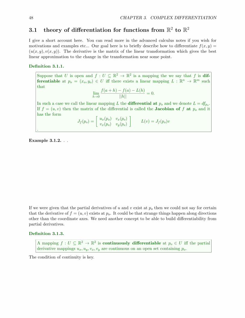
I give a short account here. You can read more in the advanced calculus notes if you wish formotivations and examples etc... Our goal here is to briefly describe how to differentiate f(x, y) =(u(x, y), v(x, y)). The derivative is the matrix of the linear transformation which gives the bestlinear approximation to the change in the transformation near some point.

Definition 3.1.1.

Suppose that U is open and f : U ⊆ ℝ2 → ℝ2 is a mapping the we say that f is dif-ferentiable at po = (xo, yo) ∈ U iff there exists a linear mapping L : ℝn → ℝm suchthat

limℎ→0

f(a+ ℎ)− f(a)− L(ℎ)

∣∣ℎ∣∣= 0.

In such a case we call the linear mapping L the differential at po and we denote L = dfpo .If f = (u, v) then the matrix of the differential is called the Jacobian of f at po and ithas the form

Jf (po) =

[ux(po) vx(po)vx(po) vy(po)

]L(v) = Jf (po)v

.

Example 3.1.2. . .

If we were given that the partial derivatives of u and v exist at po then we could not say for certainthat the derivative of f = (u, v) exists at po. It could be that strange things happen along directionsother than the coordinate axes. We need another concept to be able to build differentiability frompartial derivatives.

Definition 3.1.3.

A mapping f : U ⊆ ℝ2 → ℝ2 is continuously differentiable at po ∈ U iff the partialderivative mappings ux, uy, vx, vy are continuous on an open set containing po.

The condition of continuity is key.

3.2. COMPLEX LINEARITY 49

Theorem 3.1.4.

If f is continuously differentiable at po then f is differentiable at po

You can find the proof in Edwards on pages 72-73. This is not a trivial theorem.

Example 3.1.5. . .

3.2 complex linearity

Finally, note that we have L(cv) = cL(v) for all c ∈ ℝ in the context of the definitions and theoremsthus far in this section. The linearity is with respect to ℝ. In contrast, if we has some functionT : ℂ→ ℂ such that

(1.) T (v + w) = T (v) + T (w) for all v, w ∈ ℂ (2.) T (cv) = cT (v) for all c, v ∈ ℂ

then we would say that T is complex-linear. Condition (1.) is additivity whereas condition (2.)is homogeneity. Note that complex linearity implies real linearity however the converse is nottrue.

Example 3.2.1. . .


Suppose that L is a linear mapping from ℝ2 to ℝ2. It is known from linear algebra that there exists

a matrix A =

(a bc d

)such that L(v) = Av for all v ∈ ℝ2.

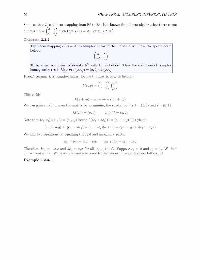
Theorem 3.2.2.

The linear mapping L(v) = Av is complex linear iff the matrix A will have the special formbelow: (

a b−b a

)To be clear, we mean to identify ℝ2 with ℂ as before. Thus the condition of complexhomogeneity reads L((a, b) ∗ (x, y)) = (a, b) ∗ L(x, y)

Proof: assume L is complex linear. Define the matrix of L as before:

L(x, y) =

(a bc d

)(xy

)This yields,

L(x+ iy) = ax+ by + i(cx+ dy)

We can gain conditions on the matrix by examining the special points 1 = (1, 0) and i = (0, 1)

L(1, 0) = (a, c) L(0, 1) = (b, d)

Note that (c1, c2) ∗ (1, 0) = (c1, c2) hence L((c1 + ic2)1) = (c1 + ic2)L(1) yields

(ac1 + bc2) + i(cc1 + dc2) = (c1 + ic2)(a+ ic) = c1a− c2c+ i(c1c+ c2a)

We find two equations by equating the real and imaginary parts:

ac1 + bc2 = c1a− c2c cc1 + dc2 = c1c+ c2a

Therefore, bc2 = −c2c and dc2 = c2a for all (c1, c2) ∈ ℂ. Suppose c1 = 0 and c2 = 1. We findb = −c and d = a. We leave the converse proof to the reader. The proposition follows. □

Example 3.2.3. . .

3.3. COMPLEX DIFFERENTIABILITY AND THE CAUCHY RIEMANN EQUATIONS 51

3.3 complex differentiability and the Cauchy Riemann equations

In analogy with the real case we could define f ′(z) as the slope of the best complex-linearapproximation to the change in f near z. This is equivalent to the following definition:

Definition 3.3.1.

Suppose f : dom(f) ⊆ ℂ→ ℂ and z ∈ dom(f) then we define f ′(z) by the limit below:

f ′(z) = limℎ→0

f(z + ℎ)− f(z)

ℎ.

The derivative function f ′ is defined pointwise for all such z ∈ dom(f) that the limit aboveexists.

Note that f ′(z) = limℎ→0f ′(z)ℎℎ hence

limℎ→0

f ′(z)ℎ

ℎ= lim

ℎ→0

f(z + ℎ)− f(z)

ℎ⇒ lim

ℎ→0

f(z + ℎ)− f(z)− f ′(z)ℎℎ

= 0

Note that the limit above simply says that L(v) = f ′(z)v gives the is the best complex-linearapproximation of Δf = f(z + ℎ)− f(z).

Proposition 3.3.2.

If f is a complex differentiable at zo then linearization L(ℎ) = f ′(zo)ℎ is a complex linearmapping.

Proof: let c, ℎ ∈ ℂ and note L(cℎ) = f ′(zo)(cℎ) = cf ′(zo)ℎ = cL(ℎ). □

The difference between the definitions of L(ℎ) = f ′(zo)ℎ and L(v) = Jf (po)v ( see Definition 3.1.1)is that in the complex derivative we divide by a small complex number whereas in the derivativeof f : ℝ2 → ℝ2 we divided by the norm of a two-dimensional vector1.

Proposition 3.3.3.

If f is a complex differentiable at zo then f is (real) differentiable at zo with L(ℎ) = f ′(zo)ℎ.

Proof: note that limℎ→0f(z+ℎ)−f(z)−f ′(z)ℎ

ℎ = 0 implies

limℎ→0

f(z + ℎ)− f(z)− f ′(z)ℎ∣ℎ∣

= 0

but then ∣ℎ∣ = ∣∣ℎ∣∣ and we know L(ℎ) = f ′(zo)ℎ is real-linear hence L is the best linear approxi-mation to Δf at zo and the proposition follows. □

1note that the definition of the derivative for f : ℝn → ℝm is the same but Jf (po) is then a m × n matrix ofpartials in the general case. Each row is the gradient vector of a component function, in the case n = 1 the Jacobianmatrix gives us the gradient of the function; Jf = (∇f)T .


Let’s summarize what we’ve learned: if f : dom(f) → ℂ is complex differentiable at zo andf = u+ iv then,

1. L(ℎ) = f ′(zo)ℎ is complex linear.

2. L(ℎ) = f ′(zo)ℎ is the best real linear approximation to f viewed as a mapping on ℝ2.

The Jacobian matrix for f = (u, v) has the form

Jf (po) =

[ux(po) uy(po)vx(po) vy(po)

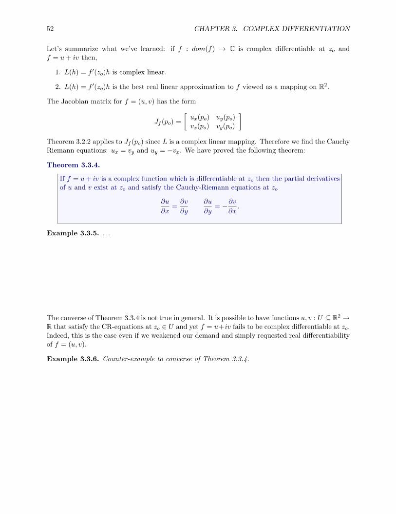
]Theorem 3.2.2 applies to Jf (po) since L is a complex linear mapping. Therefore we find the CauchyRiemann equations: ux = vy and uy = −vx. We have proved the following theorem:

Theorem 3.3.4.

If f = u+ iv is a complex function which is differentiable at zo then the partial derivativesof u and v exist at zo and satisfy the Cauchy-Riemann equations at zo

∂u

∂x=∂v

∂y

∂u

∂y= −∂v

∂x.

Example 3.3.5. . .

The converse of Theorem 3.3.4 is not true in general. It is possible to have functions u, v : U ⊆ ℝ2 →ℝ that satisfy the CR-equations at zo ∈ U and yet f = u+iv fails to be complex differentiable at zo.Indeed, this is the case even if we weakened our demand and simply requested real differentiabilityof f = (u, v).

Example 3.3.6. Counter-example to converse of Theorem 3.3.4.


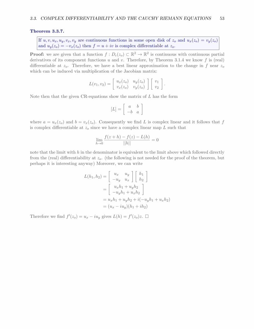
Theorem 3.3.7.

If u, v, ux, uy, vx, vy are continuous functions in some open disk of zo and ux(zo) = vy(zo)and uy(zo) = −vx(zo) then f = u+ iv is complex differentiable at zo.

Proof: we are given that a function f : D�(zo) ⊂ ℝ2 → ℝ2 is continuous with continuous partialderivatives of its component functions u and v. Therefore, by Theorem 3.1.4 we know f is (real)differentiable at zo. Therefore, we have a best linear approximation to the change in f near zowhich can be induced via multiplication of the Jacobian matrix:

L(v1, v2) =

[ux(zo) uy(zo)vx(zo) vy(zo)

] [v1

v2

].

Note then that the given CR-equations show the matrix of L has the form

[L] =

[a b−b a

]where a = ux(zo) and b = vx(zo). Consequently we find L is complex linear and it follows that fis complex differentiable at zo since we have a complex linear map L such that

limℎ→0

f(z + ℎ)− f(z)− L(ℎ)

∣∣ℎ∣∣= 0

note that the limit with ℎ in the denominator is equivalent to the limit above which followed directlyfrom the (real) differentiability at zo. (the following is not needed for the proof of the theorem, butperhaps it is interesting anyway) Moreover, we can write

L(ℎ1, ℎ2) =

[ux uy−uy ux

] [ℎ1

ℎ2

]=

[uxℎ1 + uyℎ2

−uyℎ1 + uxℎ2

]= uxℎ1 + uyℎ2 + i(−uyℎ1 + uxℎ2)

= (ux − iuy)(ℎ1 + iℎ2)

Therefore we find f ′(zo) = ux − iuy gives L(ℎ) = f ′(zo)z. □


3.3.1 how to calculate df/dz via partial derivatives of components

If the partials exist and are continuous near a point zo and satisfy the CR-equations then we havea few nice formulas to calculate f ′(z):

f ′(z) = ux + ivx f ′(z) = vy − iuy f ′(z) = ux − iuy f ′(z) = vy + ivx

Example 3.3.8. . .

Example 3.3.9. . .

Example 3.3.10. . .


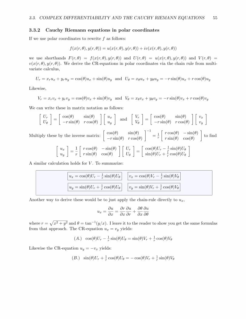
3.3.2 Cauchy Riemann equations in polar coordinates

If we use polar coordinates to rewrite f as follows:

f(x(r, �), y(r, �)) = u(x(r, �), y(r, �)) + iv(x(r, �), y(r, �))

we use shorthands F (r, �) = f(x(r, �), y(r, �)) and U(r, �) = u(x(r, �), y(r, �)) and V (r, �) =v(x(r, �), y(r, �)). We derive the CR-equations in polar coordinates via the chain rule from multi-variate calculus,

Ur = xrux + yruy = cos(�)ux + sin(�)uy and U� = x�ux + y�uy = −r sin(�)ux + r cos(�)uy

Likewise,

Vr = xrvx + yrvy = cos(�)vx + sin(�)vy and V� = x�vx + y�vy = −r sin(�)vx + r cos(�)vy

We can write these in matrix notation as follows:[UrU�

]=

[cos(�) sin(�)−r sin(�) r cos(�)

] [uxuy

]and

[VrV�

]=


] [vxvy

]

Multiply these by the inverse matrix:


]−1

= 1r

[r cos(�) − sin(�)r sin(�) cos(�)

]to find

[uxuy

]=

1

r

[r cos(�) − sin(�)r sin(�) cos(�)

] [UrU�

]=

[cos(�)Ur − 1

r sin(�)U�sin(�)Ur + 1

r cos(�)U�

]A similar calculation holds for V . To summarize:

ux = cos(�)Ur − 1r sin(�)U� vx = cos(�)Vr − 1

r sin(�)V�

uy = sin(�)Ur + 1r cos(�)U� vy = sin(�)Vr + 1

r cos(�)V�

Another way to derive these would be to just apply the chain-rule directly to ux,

ux =∂u

∂x=∂r

∂x

∂u

∂r+∂�

∂x

∂u

∂�

where r =√x2 + y2 and � = tan−1(y/x). I leave it to the reader to show you get the same formulas

from that approach. The CR-equation ux = vy yields:

(A.) cos(�)Ur − 1r sin(�)U� = sin(�)Vr + 1

r cos(�)V�

Likewise the CR-equation uy = −vx yields:

(B.) sin(�)Ur + 1r cos(�)U� = − cos(�)Vr + 1

r sin(�)V�


Multiply (A.) by r sin(�) and (B.) by r cos(�) and subtract (A.) from (B.):

U� = −rVr

Likewise multiply (A.) by r cos(�) and (B.) by r sin(�) and add (A.) and (B.):

rUr = V�

Finally, recall that z = rei� = r(cos(�) + i sin(�)) hence

f ′(z) = ux + ivx

= (cos(�)Ur − 1r sin(�)U�) + i(cos(�)Vr − 1

r sin(�)V�)

= (cos(�)Ur + sin(�)Vr) + i(cos(�)Vr − sin(�)Ur)

= (cos(�)− i sin(�))Ur + i(cos(�)− i sin(�))Vr

= e−i�(Ur + iVr)

Theorem 3.3.11.

If f(rei�) = U(r, �) + iV (r, �) is a complex function written in polar coordinates r, � thenthe Cauchy Riemann equations are written U� = −rVr and rUr = V�. If f ′(zo) exists thenthe CR-equations in polar coordinates hold. Likewise, if the CR-equations hold in polarcoordinates and all the polar component functions and their partial derivatives with respectto r, � are continuous on an open disk about zo then f ′(zo) exists and f ′(z) = e−i�(Ur+iVr).

Example 3.3.12. . .

Example 3.3.13. . .

3.4. ANALYTIC FUNCTIONS 57

3.4 analytic functions

In the preceding section we found necessary and sufficient conditions for the component functionsu, v to construct an complex differentiable function f = u + iv. The definition that follows is thenext logical step: we say a function is analytic2 at zo if it is complex differentiable at each point insome open disk about zo.

Definition 3.4.1.

Let f = u + iv be a complex function. If there exists � > 0 such that f is complexdifferentiable for each z ∈ D�(zo) then we say that f is analytic at zo. If f is analytic foreach zo ∈ U then we say f is analytic on U . If f is not analytic at zo then we say that zois a singular point. Singular points may be outside the domain of the function. If f isanalytic on the entire complex plane then we say f is entire. Analytic functions arealso called holomorphic functions

The theorem below shows that the sum, difference, quotient, product and composite of analyticfunctions is again analytic provided that there is no division by zero in the expresssion. This meansthat polynomials will be analytic everywhere, rational functions will be analytic at points where thedenominator is nonzero and similar comments apply to algebraic functions of a complex variable.For the most part singular points will arise from division by zero in later examples.

Theorem 3.4.2.

Suppose f, g are complex differentiable at z ∈ ℂ and c ∈ ℂ then

1. ddz (f(z) + g(z)) = df

dz + dgdz

2. ddz (f(z)g(z)) = df

dzg(z) + f(z)dgdz

3. if g(z) ∕= 0 then ddz

[ f(z)g(z)

]= f ′(z)g(z)−f(z)g′(z)

g(z)2

4. ddz (cf) = c dfdz

5. if ℎ is differentiable at f(z) then ddz (ℎ(f(z))) = dℎ

dzdfdz = ℎ′(f(z))f ′(z)

6. ddz (c) = 0

7. ddz (zn) = nzn−1 for n ∈ ℕ

8. ddz (ez) = ez

2you may recall that a function on ℝ was analyic at xo if its Talyor series at xo converged to the function in someneighborhood of xo. This terminology is consistent but it’ll be while before we make the connection explicit


Proof: I use Proposition 2.2.8 to simplify limits throughout the argument below. That propositionhelps us avoid direct �− � argumentation. Assume f, g are differentiable at z then

limℎ→0

f(z + ℎ) + g(z + ℎ)− f(z)− g(z)

ℎ= lim

ℎ→0

f(z + ℎ)− f(z)

ℎ+ limℎ→0

g(z + ℎ)− g(z)

ℎ

= f ′(z) + g′(z).

This proves (1.). I leave the of the other parts (2-7) as exercises for the reader. To prove (8.) recallthat ez = ex cos(y) + iex sin(y) for z = x+ iy. Note that the Cauchy Riemann equations are indeedsatisfied by u(x, y) = ex cos(y) and v(x, y) = ex sin(y) since

ux = u, uy = −v, vx = v, vy = u

gives ux = vy and uy = −vx. Moreover, u, v, ux, uy, vx, vy are clearly continuous on ℂ thus we findf(z) = ez is differentiable at each z ∈ ℂ. Moreover,

f ′(z) = ux + ivx = u+ iv ⇒ d

dz(ez) = ez. □

Example 3.4.3. . .

Example 3.4.4. . .

Example 3.4.5. . .

3.4. ANALYTIC FUNCTIONS 59

Example 3.4.6. . .


Theorem 3.4.7.

If f : U ⊆ ℂ→ ℂ is complex differentiable at zo then f is continuous at zo. Moreover, if fis analytic at zo then there exists an open disk D�(zo) on which f is continuous.

Proof: We seek to show that limℎ→0 f(zo + ℎ) = f(zo). Consider that

limℎ→0

f(zo + ℎ) = f(zo) ⇔ limℎ→0

(f(zo + ℎ)− f(zo)) = 0

⇔ limℎ→0

ℎ(f(zo + ℎ)− f(zo))

ℎ= 0

⇔ limℎ→0

(ℎ) limℎ→0

f(zo + ℎ)− f(zo)

ℎ= 0

⇔ 0 ⋅ f ′(zo) = 0

The last statement is clearly true and the limit properties clearly hold because all the limits statedin the calculation exist. Finally, if f is analytic at zo then it follows that there exists an open diskD�(zo) such that f is differentiable at each point in the disk. But then f is continuous at eachpoint as well by the first part of the theorem. □

The contrapositive of the theorem above indicates that if there does not exist at least one opendisk on which the function is continuous then the function is not analytic at that point. It followsthat we have to throw out some of the domain of the branches we’ve used for the root function orthe principal argument. To avoid discontinuity we must throw out the branch entirely.

Example 3.4.8. The princpal square root function is defined by f1(z) = ∣z∣exp(iArg(z)/2). Thedomain of f1 is governed by the princpal argument; dom(f) = {z ∈ ℂ ∣ z ∕= 0} However, Arg(z) = �gives points of discontinuity since

f1(z) = ∣z∣exp(iArg(z)/2) = ∣z∣(cos(Arg(z)/2) + isin(Arg(z)/2))

has f1(z) → ∣z∣ sin(�/2) = ∣z∣ for paths with Arg(z) → � whereas f1(z) → ∣z∣ sin(−�/2) = −∣z∣for paths with Arg(z) → −�. We must remove Arg(z) = � from the domain if we wish f1 to beanalytic.

Example 3.4.9. Note, f(z) = Arg(z) is analytic if we restrict to

dom(f) = {z ∈ ℂ ∣ if Im(z) = 0 then Re(z) ≰ 0}.

In other words, dom(f) = ℂ− negative real axis and origin.

Similar comments apply to various branches of the logarithm and the n − tℎ root mapping. Thekey is that continuity is required for an analytic function. However, continuity is not a sufficientcondition for analyticity.

3.5. DIFFERENTIATION OF COMPLEX VALUED FUNCTIONS OF A REAL VARIABLE 61

Theorem 3.4.10.

If f is analytic on a domain D and f ′(z) = 0 for all z ∈ D then f is constant on D.

Proof: let a, b ∈ D and, by connectedness of D, consider the line segment [a, b] ⊂ D parametrizedby (t) = a + t(b − a) for 0 ≤ t ≤ 1. Note, f ∘ : [0, 1] → [a, b] → ℂ. The generalized chain rulestates that the differential of the composite of two functions is the composite of the differentials,

dt(f ∘ ) = d (t)f ∘ dt

But, f ′(z) = 0 for all z ∈ D implies d (t)f(ℎ) = f ′( (t))ℎ = 0 for all ℎ ∈ ℂ. Thus d (t)f = 0 whichgives us dt(f ∘ ) = 0. It follows that, if f = u + iv then df = (df/dt)dt = (du/dt + idv/dt)dt = 0thus,

ddt(u( (t))) = 0 and d

dt(v( (t))) = 0

for all t ∈ [0, 1]. But then u([a, b]) = {uo} and v([a, b]) = {vo} and we find that f([a, b]) = uo + ivoso the function is constant along the line segment in D. But, if D is connected then we can connectany two points p, q by a sequence of line segments and each line segment remains in D hence thevalue of the function is constant on each line segement. It follows that the function has f(p) = f(q)for all p, q ∈ D thus f(D) = {uo + ivo}. □

3.5 differentiation of complex valued functions of a real variable

Perhaps some of the concepts in the proofs of Theorem 3.4.10 above seemed bizarre. In this sectionwe take some time to derive the chain rule for complex-valued functions of a real variable with ananalytic complex function. We’ll conclude this section with a few comments which reflect on thelogical necessity of the complex exponential function3. Let me point out that differentiation of acomplex-valued function of a real variable is nothing more than differentiation of a two-dimensionalspace curves in calculus III. We just use a complex notation for two-dimensional real vectors in thiscourse. Let f⃗(t) =< u(t), v(t) > for t ∈ ℝ then

d

dt[ f⃗(t) ] =< du

dt ,dvdt >

In complex notation, f = u + iv and dfdt = du

dt + idvdt . The criteria for the existence of df/dt forf : ℝ→ ℂ is much weaker than the criteria for the existence of df/dz for f : ℂ→ ℂ.

Example 3.5.1. Note, f(z) = z is not analytic so f ′(z) is not defined. However, if (t) = t+ it2

then (f ∘ )(t) = f(t+ it2) = t− itt and

ddt [ (f ∘ )(t) ] = d

dt [ t− it2 ] = dt

dt − idt2

dt = 1− 2it.

3you could take this section as motivation for the complex exponential we defined earlier, this section is notlogically necessary to earlier calculations however it might give you some idea of why the complex exponential wasdefined as it was. Another motivation comes from the extension of power series to the complex setting, we’ll see thatlater on


Suppose f = u+ iv is analytic and and let (t) = a(t) + ib(t) for each t ∈ ℝ where a, b : ℝ→ ℝ. Ifwe compose f with then f ∘ : ℝ→ ℂ and we can calculate

ddt [ (f ∘ )(t) ] = d

dt [ u( (t)) + iv( (t)) ]

= ddt [ u(a(t), b(t)) + iv(a(t), b(t)) ]

= ddt [ u(a(t), b(t)) ] + i ddt [ v(a(t), b(t)) ]

= uxdadt + uy

dbdt + i[ vx

dadt + vy

dbdt ]

= (ux + ivx)dadt − i(uy + ivy)idbdt

= ∂f∂x

dadt − i

∂f∂y i

dbdt

= f ′( (t))dadt + f ′( (t))idbdt

= f ′( (t))(dadt idbdt )

= f ′( (t))d dt

We could omit the arguments as is often done in the statement of a chain rule and simply say that

ddt [ f(z(t) ] = df

dzdzdt

I remind the reader that the formula above holds for analytic functions.

Theorem 3.5.2.

Let f(t) = exp(�t) for all t ∈ ℝ then df/dt = �exp(�t).

Proof: Observe that (t) = �t = Re(�)t+ iIm(�)t has d /dt = Re(�)+ iIm(�) and f(z) = exp(z)has df/dz = exp(z) therefore, by the calculation preceding the theorem, d/dt(exp(�t)) = �exp(�t).

Some authors might motivate the definition of the complex exponential function by assuming itshould satisfy the theorem above. However you choose the starting point we should all agree thatthe complex exponential function should reduce to the real exponential function when restrictedto the real-axis and it should maintain as many properties of the real exponential function as isreasonably possible in the complex setting. Indeed this is how all complex functions are typicallydefined. We want two main things: to extend f : ℝ→ ℝ to f̃ : ℂ→ ℂ we expect

1. f̃ ∣ℝ = f

2. interesting properties of f generalize to properties of f̃ .

Item (2.) is where the fun is. We’ll see how to define complex trigonmetric and hyperbolic functionsin the upcoming sections. I suspect it’s worth noting that one problem that naturally suggests thedefinition of the complex exponential is the problem of 2nd order ordinary-constant-coefficientdifferential equations: that is, suppose you want to solve:

ay′′ + by′ + cy = 0

3.5. DIFFERENTIATION OF COMPLEX VALUED FUNCTIONS OF A REAL VARIABLE 63

Since this analagous to y′ = �y which has solution y = e�t it’s natural to guess the solution hasthe form y = e�t. Clearly, y′ = �e�t and y′′ = �2e�t hence

ay′′ + by′ + cy = 0 ⇒ a�2e�t + b�e�t + c�e�t = (a�2 + b�+ c)e�t = 0

Therefore we find a necessary condition on � is that it satisfy the characteristic equation:

y = e�t solves ay′′ + by′ + cy = 0 ⇒ a�2 + b�+ c = 0.

Apparently, solving the differential equation ay′′ + by′ + cy = 0 reduces to the problem of solvinga corresponding algebra equation. Notice that we are tempted to answer the question of whata complex exponential is in this setting. Whether or not we began this discussion with complexthings in mind the math has brought us an equation which necessarily includes complex cases.Moreover, it’s easy to see that y′′ + y = 0 has y = sin(t) and y = cos(t) as solutions. Note thaty′′ + y = 0 gives �2 + 1 = 0 which has solutions � = ±i. We then must suspect that the complexexponential function has something to do with sine and cosine. The founders of complex analysiswere well aware of these sort of differential equations and it is likely that many of the complexfunctions first found their home inside some differential equation where they naturally arise as partof some general ansatz.


3.6 analytic continuations

We do not yet have the tools to prove the following statement. I postpone the proof for now.

Conjecture 3.6.1.

If f is analytic on a disk D1 and f(z) = 0 for all z ∈ S where S is either a line-segment oranother disk contined in D1 then f(z) = 0 for all z ∈ D1.

Note we can extend this to a domain without too much trouble.

Theorem 3.6.2.

If f is analytic on a domain D and if f(z) = 0 for all z ∈ S where S is either a line-segmentor another disk contined in D then f(z) = 0 for all z ∈ D.

Proof: Let zo ∈ S and pick w ∈ D − S. Since D is connected there exists a polygonal path = [z0, z1] ∪ [z1, z2] ∪ ⋅ ⋅ ⋅ ∪ [zn−1, w] where each of the line segments lies inside D. Let � be thesmallest distance between a point on L and the boundary of D. Construct disks of radius � withcenters separated by a distance � all along L. Notice that D is open so even the closest open diskwill not get to the edge of D (which is not contained in the open set D). Moreover, the rest of thedisks also remain in D. By our conjecture we find that the disk which is partially in S must havef identically zero since we can find a smaller disk totally in S so the conjecture gives us f zero onthe first disk partly outside S. Then we can continue this process to the next disk. We simply takea smaller disk in the intersection of the two disks and because we already know it is zero from thelast step of the argument it follows by the conjecture that f is zero on the second disk. Let mesketch a picture of the argument above:

As you can see, the argument can be repeated until we reach the disk containing w. Thus we findf(w) = 0 for arbitrary w ∈ D hence f(D) = {0}. □Theorem 3.6.3.

Let Ω be a domain or a line segment. If f is analytic on a domain D which contains Ω thenf is uniquely determined by its values on Ω.

Proof: Suppose f and g are analytic on D and f(z) = g(z) for all z ∈ Ω. Notice that ℎ : D → ℂdefined by ℎ = f − g is identically zero on Ω since ℎ(z) = f(z)− g(z) = 0 for all z ∈ Ω. But thenby 3.6 we find ℎ(z) = 0 for all z ∈ D. It follows that f = g. □

We say that f is the analytic continuation of f ∣Ω. There is more to learn and say about analyticcontinuations in general, however we have what we need for our purposes at this point. Let’s getto the point:

3.7. TRIGONOMETRIC AND HYPERBOLIC FUNCTIONS 65

Theorem 3.6.4.

If f : ℝ→ ℝ ⊂ ℂ is a function and f̃ : ℂ→ ℂ is an extension of f which is analytic thenf̃ is unique. In particular, if there is an analytic extension of sine, cosine, hyperbolic sineor hyperbolic cosine then those extensions are unique.

This means if we demand analyticity then we actually had no freedom in our choice of the exponen-tial. If we find a complex function which matches the exponential function on a line-segment ( inparticular a closed interval in ℝ viewed as a subset of ℂ is a line-segment ) then there is just onecomplex function which agrees with the real exponential and is complex differentiable everywhere.

f(x) = ex extends uniquely to f̃(z) = eRe(z)(cos(Im(z)) + i sin(Im(z))).

Note f̃(x + 0i) = ex(cos(0) + i sin(0)) = ex thus f̃ ∣ℝ = f . Naturally, analyiticity is a desireableproperty for the complex-extension of known functions so this concept of analytic continuation isvery nice. Existence aside, we should first construct sine, cosine etc... then we have to check theyare both analytic and also that they actually agree with the real sine or cosine etc... If a functionon ℝ has vertical asymptotes, points of discontinuity or points where it is not smooth then thestory is more complicated.

3.7 trigonometric and hyperbolic functions

Recall we found that for � ∈ ℝ the formulas cos(�) = 12

(ei� +e−i�

)and sin(�) = 1

2i

(ei�−e−i�

)were

useful for deriving trigonmetric identities. We now extend to complex arguments.

Definition 3.7.1.

We define cos(z) = 12

(eiz + e−iz

)and sin(z) = 1

2i

(eiz − e−iz

)for all z ∈ ℂ

Note that cos(z) and sin(z) are sums of composites of analytic functions since the function g(z) = czis clearly analytic and ℎ(z) = ez is analytic. Moreover, it is clear that f̃(z) = cos(z) restricts tothe usual real cosine function along the real axis. This is a consequence of Euler’s formula:

cos(x+ i0) = 12

(eix + e−ix

)= 1

2

(cos(x) + i sin(x) + cos(x) + i sin(−x)

)= cos(x)

Don’t get lost in the notation here, the ”cos” on the left is the newly defined complex cosine whereasthe ”cos” on the right is the cosine you know and love from the study of circular functions. Thefact that the complex cosine is the unique analytic continuation of the real cosine function makesthis notation reasonable. Similar comments apply to the sine function.


Proposition 3.7.2.

Let z ∈ ℂ,

1. sin(z) and cos(z) are unbounded.

2. sin(z) is an odd function of z

3. cos(z) is an even function of z

Notice that z = iy gives cos(z) = cos(iy) = 12

(e−y + ey

). Thus the complex cosine can assume

arbitrarily large values. Likewise, sin(iy) = 12i

(e−y − ey

)has ∣ sin(iy)∣ take arbitrarily large values

as we range over the complex plane. Items (2.) and (3.) are immediate from the definition.

Proposition 3.7.3.

Let z, w ∈ ℂ,

1. sin(z + w) = sin(z) cos(w) + cos(z) sin(w)

2. cos(z + w) = cos(z) cos(w)− sin(z) sin(w)

3. sin2(z) + cos2(z) = 1

4. sin(2z) = 2 sin(z) cos(z)

5. sin2(z) = 12(1− cos(2z))

6. cos2(z) = 12(1 + cos(2z))

I leave the proof to the reader. I think some of these are homeworks in Churchill, some I may haveassigned.

Definition 3.7.4.

We define the hyperbolic cosine cosℎ(z) = 12

(ez + e−z

)and the hyperbolic sine

sinℎ(z) = 12

(ez − e−z

)for all z ∈ ℂ.

You may recall that we defined hyperbolic cosine and sine to be the even and odd parts of theexponential function respective,

ex = 12

(ex + e−x

)︸︷︷︸cosh(x)

+ 12

(ex − e−x

)︸︷︷︸sinh(x)

Clearly the complex hyperbolic functions restrict to the real exponential functions and they arealso entire since they are the sum and composite of entire functions ez and −z. It follows thatthe complex hyperbolic functions defined above are the unique analytic continuation of the realhyperbolic functions. You could probably fill a small novel with interesting formulas which areknown for hyperbolic functions. We will content ourselves to notice these three items:

3.8. HARMONIC FUNCTIONS 67

Proposition 3.7.5.

1. i sinh(iz) = sin(z)

2. cosh(iz) = cos(z)

3. cosh2(z)− sinh2(z) = 1

Finally, I should mention that the other elementary trigonometric and hyperbolic functions arelikewise defined. For example,

tan(z) = sin(z)cos(z) , tanh(z) = sinh(z)

cosh(z) , sec(z) = 1cos(z) , secℎ(z) = 1

cosh(z) .

Inverse functions may also be defined for suitably restricted functions. Of course this should notbe surprising, even in the real case we have to restrict sine, cosine and tangent in order to obtainstandard inverse functions. This is essentially the same issue as the one we were forced to deal within our discussion of branch cuts.

Proposition 3.7.6.

1. d/dz(sin(z)) = cos(z)

2. d/dz(cos(z)) = − sin(z)

3. d/dz(tan(z)) = sec2(z)

4. d/dz(sinh(z)) = cosh(z)

5. d/dz(cosh(z)) = sinh(z)

6. d/dz(tanh(z)) = secℎ2(z)

I leave the proof of these to the reader. Also, it might be interesting to study the geometry of themapping w = sin(z) and so forth. Many complex variables texts have nice pictures of the geometry,I may put some up on the projecter in lecture. The links on the webpage point you to several siteswhich explore the geometry of mappings.

3.8 harmonic functions

We’ve discussed in some depth how to determine if a given function f = u+ iv is in fact analytic.In this section we study another angle on the story. We learn that the component functionsu, v of an analytic function f = u + iv are harmonic conjugates and they satisfy the phyicallysignificant Laplace’s equation ∇2� = 0 where ∇2 = ∂2/∂x2 + ∂2/∂y2. In addition we’ll learn


that if we have one solution of Laplace’s equation then we can consider it to be the ”u” of someyet undetermined analytic function f = u + iv. The remaining function v is then constructedthrough some integration guided by the CR-equations. The construction is similar to the problemof construction of a potential function for a given conservative force in calculus III.

Proposition 3.8.1.

If f = u + iv is analytic on some domain D ⊆ ℂ then u and v are solutions of Laplace’sequation �xx + �yy = 0 on D.

Proof: since f = u + iv is analytic we know the CR-equations hold true; ux = vy and uy = −vx.Moreover, f is continuously differentiable so we may commute partial derivatives by a theoremfrom multivariate calculus. Consider

uxx + uyy = (ux)x + (uy)y = (vy)x + (−vx)y = vyx − vxy = 0

Likewise,vxx + vyy = (vx)x + (vy)y = (−uy)x + (ux)y = −uyx + uxy = 0

Of course these relations hold for all points inside D and the proposition follows. □

Example 3.8.2. Note f(z) = z2 is analytic with u = x2 − y2 and v = 2xy. We calculate,

uxx = 2, uyy = −2 ⇒ uxx + uyy = 0

Note vxx = vyy = 0 so v is also a solution to Laplace’s equation.

Now let’s see if we can reverse this idea.

Example 3.8.3. Let u(x, y) = x + c1 notice that u solves Laplace’s equation. We seek to find aharmonic conjugate of u. We need to find v such that,

∂v

∂y=∂u

∂x= 1

∂v

∂x= −∂u

∂y= 0

Integrate these equations to deduce v(x, y) = y + c2 for some constant c2 ∈ ℝ. We thus constructan analytic function f(x, y) = x+ c1 + i(y + c2) = x+ iy + c1 + ic2. This is just f(z) = z + c forc = c1 + ic2.

Example 3.8.4. Suppose u(x, y) = ex cos(y). Note that uxx = u whereas uyy = −u hence uxx +uyy = 0. We seek to find v such that

∂v

∂y=∂u

∂x= ex cos(y)

∂v

∂x= −∂u

∂y= ex sin(y)

Integrating vy = ex cos(y) with respect to y and vx = ex sin(y) with respect to x yields v(x, y) =ex sin(y). We thus construct an analytic function f(x, y) = ex cos(y) + iex sin(y). Of course weshould recognize the function we just constructed, it’s just the complex exponential f(z) = ez.

3.8. HARMONIC FUNCTIONS 69

Notice we cannot just construct an analytic function from any given function of two variables. Wehave to start with a solution to Laplace’s equation. This condition is rather restrictive. Thereis much more to say about harmonic functions, especially where applications are concerned. Mygoal here was just to give another perspective on analytic functions. Geometrically one thing wecould see without further work at this point is that for an analytic function f = u+ iv the familiesof level curves u(x, y) = c1 and v(x, y) = c2 are orthogonal. Note grad(u) =< ux, uy > andgrad(v) =< vx, vy > have

grad(u) ⋅ grad(v) = uxvx + uyvy = −uxuy + uyux = 0

This means the normal lines to the level curves for u and v are orthogonal. Hence the level curvesof u and v are orthogonal.

Chapter 4

complex integration

In this chapter I collect many interesting theorems about contour integrals. The proofs can befound in Churchill. I will focus my efforts on adding a few examples.

4.1 integrals of a complex-valued function of a real variable

Integration of functions from ℝ into ℂ follows the rule you may recall from calculus III, we integratecomponentwise.

Definition 4.1.1.

Let f : U ⊂ ℝ→ ℂ have component functions u, v : U ⊂ ℝ→ ℝ where f(t) = u(t) + iv(t).If [a, b] ⊆ U then we define ∫ b

af(t)dt =

∫ b

au(t)dt+ i

∫ b

av(t)dt.

Indefinte integrals similarly.

Example 4.1.2. Calculate the integral,∫ [cos(t) + i sin(t)

]dt =

∫cos(t) dt+ i

∫sin(t) dt

= sin(t) + c1 + i(− cos(t) + c2)

= −i[cos(t) + i sin(t)] + c1 + ic2

Thus, following the same steps just with bounds,∫ �

0

[cos(t) + i sin(t)

]dt = sin(t)

∣∣�0− i cos(t)

∣∣�0

= −2i

Notice that we can also summarize this calculation in terms of the imaginary exponential,∫eit dt = 1

i eit + c ⇒

∫ �

0eit dt = −ieit

∣∣�0

= −ie0 + iei� = −2i

71

72 CHAPTER 4. COMPLEX INTEGRATION

The preceding example illustrates a more general pattern in these sort of integrals.

Proposition 4.1.3.

Suppose f and F are complex-valued functions of a real variable such that dFdt = f(t) then∫ b

af(t) dt = F (b)− F (a) also

∫f(t) dt = F (t) + c

The proof of the proposition follows directly from the Fundamental Theorem of Calculus. Notethat if f = u+ iv and F = U + iV and dF/dt = f it follows dU/dt = u and dV/dt = v.∫ b

af(t) dt =

∫ b

au dt+ i

∫ b

av dt

= U(b)− U(a) + i(V (b)− V (a))

= F (b)− F (a)

The notation∫f(t) dt = F (t) + c is just notation to indicate F is the antidervative of f meaning

that dFdt = f . Naturally other properties of definite integrals likewise transfer to our current context:

Proposition 4.1.4.

Suppose f, g are complex-valued functions of a real variable and a, b, c, c1 ∈ ℝ such thata < b < c

1.∫ ca f(t) dt =

∫ ba f(t) dt+

∫ cb f(t) dt

2.∫ ba f(t) dt = −

∫ ab f(t) dt

3.∫ ba [ f(t) + g(t) ]dt =

∫ ba f(t) dt+

∫ ba g(t) dt

4.∫ ba c1f(t) dt = c1

∫ ba f(t) dt

here I have assumed that f, g are continuous or possibly piecewise continuous so that theintegrals above are well-defined. Properties (3.) and (4.) also hold for indefinite integrals.

The proposition below is less trivial. The chain-rule ddt(F (�(t))) = dF

dzd�dt where � : ℝ→ ℂ is path

and F : ℂ→ ℂ is analytic at �(t) justifies the proposition below:

Proposition 4.1.5.

Suppose f and F are complex functions, meaning f : dom(f)→ ℂ and F : dom(F )→ ℂ,such that dF/dz = f . Futhermore, suppose � : I ⊆ ℝ→ ℂ such that �′(t) ∕= 0 then∫ b

af(�(t))

d�

dtdt = F (�(t))

∣∣∣∣t=bt=a

4.1. INTEGRALS OF A COMPLEX-VALUED FUNCTION OF A REAL VARIABLE 73

A slight twist on the preceding proposition gives us a u-substitution theorem in our context,∫ b

af(�(t))

d�

dtdt =

∫ �(b)

�(a)f(�)d� =

∫ �(b)

�(a)

dF

dzdz = F (�(b))− F (�(a)).

Example 4.1.6. Calculate the integral,∫ [sin(t) + it2

]13(cos(t) + 2it

)dt =

∫u13 du

=1

14u14 + c

=1

14

[sin(t) + it2

]14

+c

Don’t believe me? Just differentiate the answer and see if our antiderivative returns the integrandonce differentiated.

Example 4.1.7. Calculate the integral, for � ∈ ℂ ( a constant)∫exp(�t) dt =

∫exp(�t) dt

=

∫exp(u)

du

�

=1

�exp(u) + c

=1

�exp(�t) + c

Suppose z(t) = x(t) + iy(t) then dzdt = dx

dt + idydt , it is therefore formally reasonable to write

dz = dxdt dt+ idydt dt. This is the how we implement the substitution.

Example 4.1.8. Calculate the integral,∫sin(t+ iet)(2 + i2et) dt =

∫sin(z)

dz

2:let z = t+ iet thus dz = (1 + iet)dt

= −12 cos(z) + c

= −12 cos(t+ iet) + c

Finally, the following property (proved on page 88-89 of Churchill) is important to many argumentslater: (note, w below is chosen such that the integrals exist)

Proposition 4.1.9.

Let w(t) = u(t) + iv(t) be a complex valued function of a real variable,∣∣∣∣ ∫ b

aw(t) dt

∣∣∣∣ ≤ ∫ b

a∣w(t)∣ dt and

∣∣∣∣ ∫ ∞a

w(t) dt

∣∣∣∣ ≤ ∫ ∞a∣w(t)∣ dt


4.2 contour integrals

A contour is a curve in the complex plane which can be broken into a finite number of ”smootharcs”. Contours can self-intersect, they can even have corners. However, the arcs which comprisethe contour we assume to be smooth (meaning the derivative of the arc map is nonzero) on theirinteriors.

Definition 4.2.1.

An arc is a continuous mapping from [a, b] into ℂ . A smooth arc is an arc suchthat ′(t) ∕= 0 for all t ∈ (a, b). Suppose C ⊂ ℂ such that C = C1 ∪ C2 ∪ ⋅ ⋅ ⋅ ∪ Cn andsuppose there exist smooth arcs j : [aj , bj ] → Cj where 1(a1) = p and n(bn) = q and j(bj) = j+1(aj+1) for each j = 1, 2, . . . n− 1 then we say C is a contour from terminalpoint p to terminal point q. If C is a contour which begins and ends at the same pointthen we say C is a closed contour. A simple arc is an arc which is given by an injectivearc map, it has no ”self-intersections”. Likewise, a contour is called simple if it has no self-intersections except possibly the terminal points of the contour. A simple closed contouronly intersects itself at the terminal points. Finally, for a given contour many arcs may beused to cover the contour, we call each a particular parametrization of the contour.

The Jordon curve theorem applied to the complex plane states that a simple closed contour dividesthe complex plane into a it simply connected interior and an unbounded exterior. The term simplyconnected has the same meaning as when it was discussed in your calculus III course. In a nutshell,a set is simply connected if any loop in the set can be continuously deformed to a point. For atwo-dimensional set this means it has no holes. In three dimensions, you can have a hole in a simplyconnected set.

Definition 4.2.2. integral along an arc

Let : [a, b]→ C ⊂ ℂ and suppose f : dom(f) ⊆ ℂ→ ℂ is continuous on C then∫Cf(z)dz =

∫ b

af( (t))

d

dtdt

Moreover, we may sometimes denote∫C f(z)dz =

∫C f .

I should mention that f(z) is just short for f(x, y) in the definition above. For example, we doallow for integration of f(z) = z̄.

Example 4.2.3. Suppose C is the line segment from p to q then it is an arc and we may use themap (t) = p+ t(q − p) for 0 ≤ t ≤ 1 to parameterize C. Generically,

∫C f(z)dz =

∫ 10 f(p+ t(q −

p))(p− q)dt. For example, if f(z) = z2, p = 1, q = 1 + 2i then∫Cz2 dz =

∫ 1

0(1 + 2it)2(2i)dt = 1

3(1 + 2it)3

∣∣∣∣10

= 13

[(1 + 2i)3 − 1

]= −2

3

[i+ 6

]

4.2. CONTOUR INTEGRALS 75

You might notice in the last example the parametrization seems superfluous, couldn’t we just writethe following instead?∫

Cz2 dz =

∫ 1+2i

1z2 dz = 1

3z3

∣∣∣∣1+2i

1

= 13

[(1 + 2i)3 − 1

]= −2

3

[i+ 6

]The answer: no. Not without a lot of fine print. Notice that the bounded integral was neverdefined, it begs the question what about another curve from 1 to 1 + 2i, what notation would weuse for that? Would another path give the same result? Let’s look at another example beforethinking too much about the curious (formal) calculation above.

Example 4.2.4. Suppose C is the quarter circle from 1 to i which is an arc with map (t) = eit

for 0 ≤ t ≤ �/2 to parameterize C.

∫Cz̄ dz =

∫ �2

0eit(ieit)dt =

∫ �2

0i dt = �/2.

Likewise, if we let C2 be the full unit circle then the same arc map applies and we simply need toextend the bounds to range from 0 to 2� and we could calculate

∫C z̄ dz = 2�.

Note that if there was a formal calculation that could take the place of the contour integrationabove then it would have to return a result of zero since the contour above begins and ends at thesame point. What’s the difference between the preceding pair of examples? What’s the differencebetween f(z) = z2 and g(z) = z̄? I’ll let you think about it, the answer is contained in the Theoremon page 105 of Churchill.

Definition 4.2.5. contour integration

If C = C1 ∪ C2 ∪ ⋅ ⋅ ⋅ ∪ Cn is a contour comprised of n-arcs Cj then the contour integralof a continuous complex function f : dom(f)→ ℂ such that C ⊆ dom(f) is defined as thesum of the integrals over the arcs∫

Cf(z)dz =

n∑j=1

∫Cj

f(z)dz

Often the notation C = C1 +C2 + ⋅ ⋅ ⋅Cn is used in the context above, it simply means that the arcsare placed end to end and in total they cover the contour C. Also, we can weaken the criteria ofcontinuity to piecewise continuity and the custom is just to add up the results of the pieces. Varioustexts cut this definition more or less finely. I hope I’ve given you enough detail as for it to makesense. It is possible to define it from a complex Riemann sum or in terms of the correspondance toline-integrals.

Example 4.2.6. Suppose S = C1 ∪C2 ∪C3 ∪C4 is a square which is oriented in the CCW fashion


with corners (a, b), (a+ℎ, b), (a+ℎ, b+ℎ), (a, b+ℎ). The contour integral of f(z) = z works out to∫Szdz =

∫C1

zdz +

∫C2

zdz +

∫C3

zdz +

∫C4

zdz

=

∫C1

(x+ ib)dz +

∫C2

(a+ ℎ+ iy)dz +

∫C3

(x+ i(b+ ℎ)dz +

∫C4

(a+ iy)dz

=

∫ ℎ

0

(a+ t+ ib

)dt+ i

∫ ℎ

0

(a+ ℎ+ i(b+ t)

)dt

−∫ ℎ

0

(a+ ℎ− t+ i(b+ ℎ)

)dt− i

∫ ℎ

0

(a+ i(b+ ℎ− t)

)dt

=

∫ ℎ

0

(2t− 2t− ℎ+ ℎ

)dt

= 0

The notation is very natural to calculate dz just use dz = dx + idy, this notation is equivalent toour parametric mapping definition.

1. C1 = [a+ ib, a+ ℎ+ ib] has x = a+ t and y = bso dx = dt and dy = 0 hence dz = dt.

2. C2 = [a+ ℎ+ ib, a+ ℎ+ i(b+ ℎ)] has x = a+ ℎ and y = b+ tso dx = 0 and dy = dt and dz = idt

3. C3 = [a+ ℎ+ i(b+ ℎ), a+ i(b+ ℎ)] has x = a+ ℎ− t and y = b+ ℎso dx = −dt and dy = 0 and dz = −dt

4. C4 = [a+ i(b+ ℎ), a+ ib] has x = a and y = b+ ℎ− tso dx = 0 and dy = −dt and dz = −idt

Since this was a square I was able to take 0 ≤ t ≤ ℎ on each side. For a rectangle it would benatural to follow almost the same calculation except the vertical legs and horizontal legs would havea different ℎ-value. Essentially the same cancellation will again occur. Why? (again see Theoremon page 105 and think about what makes f(z) = z special.

Proposition 4.2.7. basic properties of contour integration

1. let C be a contour and −C be the contour in the reverse direction∫−C

f(z)dz = −∫Cf(z)dz.

2. Let L be the arclength of the contour C, if ∣f(z)∣ ≤M for z ∈ C then∣∣∣∣ ∫Cf(z) dz

∣∣∣∣ ≤ML

4.3. ANTIDERIVATIVES AND ANALYTIC FUNCTIONS 77

I gave additional examples in lecture, if you missed class please get notes from a classmate. Onething I might ask you to prove is that the contour integral is well-defined. In particular, you shouldbe able to show it is invariant under a reparametrization of the contour. (if you can prove it for anarc that would be sufficient, it’s what I did in lecture.).

Apology: I would very much like to have notes written corresponding to sections 34-42of Churchill however, I don’t believe I will have time before your test, or perhaps thissemester. The text is good, we did cover these section before spring break, and if youwant good notes I would advise you to ask a student who attended all the lectures.I do hope to provide more notes but until that happens please make use of the textand perhaps my notes from when I took this course from my advisor Dr. Fulp

4.3 antiderivatives and analytic functions

4.4 Cauchy Goursat and the deformation theorems

4.5 Cauchy’s Integral Formula

4.6 Lioville’s Theorem and the Fundmental Theorem of Algebra

Chapter 5

Taylor and Laurent series

sections 43-52

79

80 CHAPTER 5. TAYLOR AND LAURENT SERIES

Chapter 6

residue theory

sections 53-59

81

82 CHAPTER 6. RESIDUE THEORY

Chapter 7

residue theory

sections 60-64

83

lecture for complex variables

Documents

phrase i

complex variablesjames

complex logarithms

complex dierentiation

notesa complex variable

history of complex numbers

theory of complex variableswas

polar form of complex