lecture abstract ee c128 / me c134 – feedback control...

EE C128 / ME C134 – Feedback Control SystemsLecture – Chapter 2 – Modeling in the Frequency Domain

Alexandre Bayen

Department of Electrical Engineering & Computer Science

University of California Berkeley

September 10, 2013

Bayen (EECS, UCB) Feedback Control Systems September 10, 2013 1 / 34

Lecture abstract

Topics covered in this presentation

I Laplace transform

I Transfer function

I Conversion between systems in time-, frequency-domain, and transferfunction representations

I Electrical, translational-, and rotational-mechanical systems in time-,frequency-domain, and transfer function representations

I Nonlinearities

I Linearization of nonlinear systems in time-, frequency-domain, andtransfer function representations


Chapter outline

1 2 Modeling in the frequency domain2.1 Introduction2.2 Laplace transform review2.3 The transfer function2.4 Electrical network transfer functions2.5 Translational mechanical system transfer functions2.6 Rotational mechanical system transfer functions2.7 Transfer functions for systems with gears2.8 Electromechanical system transfer functions2.9 Electric circuit analogs2.10 Nonlinearities2.11 Linearization


2 Modeling in the frequency domain 2.2 Laplace transform review




History interlude

Pierre-Simon LaplaceI 1749 – 1827

I French mathematician andastronomer

I Pioneered the Laplace

transform

I AKA French Newton

I “...all the e↵ects of nature areonly mathematical results of asmall number of immutablelaws.”

I “What we know is little, andwhat we are ignorant of isimmense.”



The Laplace transform definitions, [1, p. 35]

Laplace transform

L[f(t)] = F (s) =

Z 1

0�f(t)e�st

dt

Inverse Laplace transform

L�1[F (s)] =1

2⇡j

Z�+j1

��j1F (s)estds

= f(t)u(t)

wheres = � + j!



Laplace transform table, [1, p. 36]

f(t) F (s)

�(t) 1

u(t)

1s

tu(t)

1s2

t

nu(t)

n!sn+1

e

�atu(t)

1s+a

sin(!t)u(t)

!s2+!2

cos(!t)u(t)

ss2+!2

e

�atsin(!t)u(t)

!(s+a)2+!2

e

�atcos(!t)u(t)

s+a(s+a)2+!2



Laplace transform theorems, [1, p. 37]

Some basic algebraic operations, such as multiplication by exponentialfunctions or shifts have simple counterparts in the Laplace domain

Theorem (Frequency shift)

L[e�at

f(t)] = F (s+ a)

Theorem (Time shift)

L[f(t� T )] = e

�sT

F (s)




Theorem (Linearity)

L[c1

f

1

(t) + c

2

f

2

(t)] = c

1

F

1

(s) + c

2

F

2

(s)

Theorem (Scaling)

L[f(at)] = 1

a

F

�s

a

�




Theorem (Di↵erentiation)

L ⇥d

nf

dt

n

⇤= s

n

F (s)�nX

k=1

s

n�k

d

k�1

f

dt

k�1

(0�)

Examples

L ⇥df

dt

⇤= sF (s)� f(0�)




Theorem (Integration)

LhR

t

0� f(⌧)d⌧i=

F (s)

s




Theorem (Final value)

L[f(1)] = lims!0

sF (s)

To yield correct finite results, all roots of the denominator of F (s) must

have negative real parts, and no more than one can be at the origin.




Theorem (Initial value)

L[f(0+)] = lims!1

sF (s)

To be valid, f(t) must be continuous or have a step discontinuity at t = 0,i.e., no impulses or their derivatives at t = 0.



Partial fraction expansion, [1, p. 37]

To find the inverse Laplace transform of a complicated function, we canconvert the function to a sum of simpler terms for which we know theLaplace transform of each term

F (s) =N(s)

D(s)

How F (s) can be expanded is governed by the relative order betweenN(s) and D(s)

1. O(N(s)) < O(D(s))

2. O(N(s)) � O(D(s))

and the type of roots of D(s)

1. Real and distinct

2. Real and repeated

3. Complex or imaginary


2 Modeling in the frequency domain 2.3 The TF



2 Modeling in the frequency domain 2.3 The TF

The transfer function, [1, p. 44]

General n-th order, linear, time-invariant di↵erential equation

a

n

d

n

c(t)

dt

n

+ a

n�1

d

n�1

c(t)

dt

n�1

+ ...+ a

0

c(t) =

b

m

d

m

r(t)

dt

m

+ b

m�1

d

m�1

r(t)

dt

m�1

+ ...+ b

0

r(t)

Under the assumption that all initial conditions are zero the transferfunction (TF) from input, c(t), to output, r(t), i.e., the ratio of the outputtransform, C(s), divided by the input transform, R(s) is given by

G(s) =C(s)

R(s)=

b

m

s

m + b

m�1

s

m�1 + ...+ b

0

a

n

s

n + a

n�1

s

n�1 + ...+ a

0

Also, the output transform, C(s) can be written as

C(s) = R(s)G(s)


2 Modeling in the frequency domain 2.4 Electrical network TFs




Electrical network TFs, [1, p. 47]

Table: Voltage-current, voltage-charge, and impedance relationships forcapacitors, resistors, and inductors




Example(Resistor-inductor-capacitor (RLC)system)

IProblem: Find the TF relatingthe capacitor voltage, V

C

(s),to the input voltage, V (s)

ISolution: On board

Figure: RLC system




Example (Inverting operationalamplifier system)

IProblem: Find the TF relatingthe output voltage, V

o

(s), tothe input voltage V

i

(s)

ISolution: On board

Figure: Inverting operational amplifiersystem


2 Modeling in the frequency domain 2.5 Translational mechanical system TFs




Translational mechanical system TFs, [1, p. 61]

Table: Force-velocity, force-displacement, and impedance translationalrelationships for springs, viscous dampers, and mass



Translational mechanical system TFs, [1, p. 63]

Example (Translationalinertia-spring-damper system)

IProblem: Find the TF relatingthe position, X(s), to theinput force, F (s)

ISolution: On board

Figure: Physical system; block diagram


2 Modeling in the frequency domain 2.6 Rotational mechanical system TFs




Rotational mechanical system TFs, [1, p. 69]

Table: Torque-angular velocity, torque-angular displacement, and impedancerotational relationships for springs, viscous dampers, and inertia



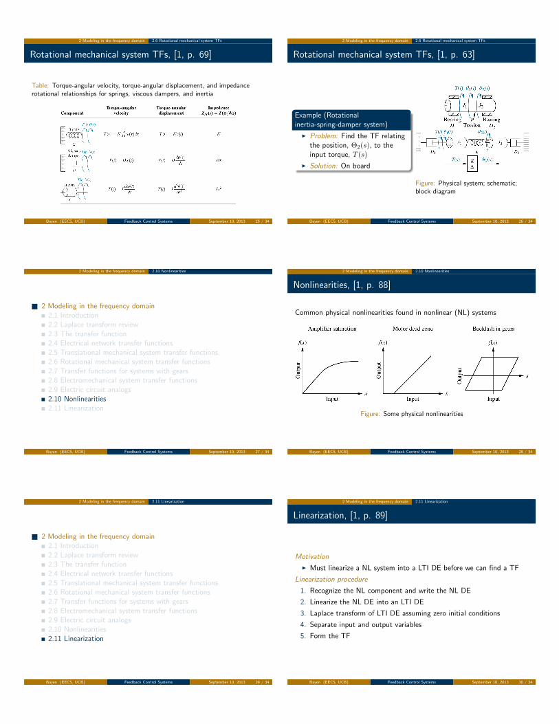
Rotational mechanical system TFs, [1, p. 63]

Example (Rotationalinertia-spring-damper system)

IProblem: Find the TF relatingthe position, ⇥

2

(s), to theinput torque, T (s)

ISolution: On board

Figure: Physical system; schematic;block diagram


2 Modeling in the frequency domain 2.10 Nonlinearities



2 Modeling in the frequency domain 2.10 Nonlinearities

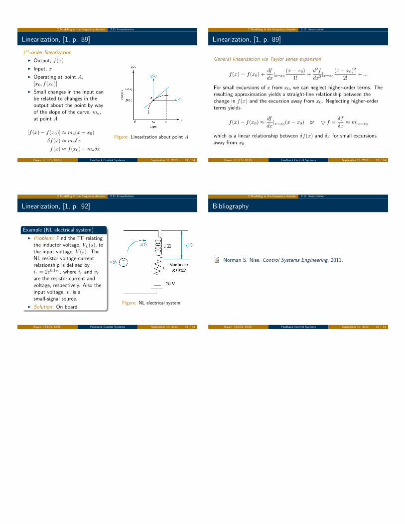
Nonlinearities, [1, p. 88]

Common physical nonlinearities found in nonlinear (NL) systems

Figure: Some physical nonlinearities


2 Modeling in the frequency domain 2.11 Linearization




Linearization, [1, p. 89]

Motivation

I Must linearize a NL system into a LTI DE before we can find a TF

Linearization procedure

1. Recognize the NL component and write the NL DE

2. Linearize the NL DE into an LTI DE

3. Laplace transform of LTI DE assuming zero initial conditions

4. Separate input and output variables

5. Form the TF




1st-order linearization

I Output, f(x)

I Input, x

I Operating at point A,[x

0

, f(x0

)]

I Small changes in the input canbe related to changes in theoutput about the point by wayof the slope of the curve, m

a

,at point A

[f(x)� f(x0

)] ⇡ m

a

(x� x

0

)

�f(x) ⇡ m

a

�x

f(x) ⇡ f(x0

) +m

a

�x

Figure: Linearization about point A




General linearization via Taylor series expansion

f(x) = f(x0

) +df

dx

|x=x0

(x� x

0

)

1!+

d

2

f

dx

2

|x=x0

(x� x

0

)2

2!+ ...

For small excursions of x from x

0

, we can neglect higher-order terms. Theresulting approximation yields a straight-line relationship between thechange in f(x) and the excursion away from x

0

. Neglecting higher-orderterms yields

f(x)� f(x0

) ⇡ df

dx

|x=x0(x� x

0

) or 5 f =�f

�x

⇡ m|x=x0

which is a linear relationship between �f(x) and �x for small excursionsaway from x

0

.




Example (NL electrical system)

IProblem: Find the TF relatingthe inductor voltage, V

L

(s), tothe input voltage, V (s). TheNL resistor voltage-currentrelationship is defined byi

r

= 2e0.1vr , where i

r

and v

r

are the resistor current andvoltage, respectively. Also theinput voltage, v, is asmall-signal source.

ISolution: On board

Figure: NL electrical system



Bibliography

Norman S. Nise. Control Systems Engineering, 2011.


lecture abstract ee c128 / me c134 – feedback control...

Documents