Lecture 9-1Analysis of Variance

General ANOVA Setting

• Investigator controls one or more independent variables– Called factors (or treatment variables)– Each factor contains two or more levels (or

categories/classifications)

• Observe effects on dependent variable– Response to levels of independent variable

• Experimental design: the plan used to test hypothesis

Completely Randomized Design

• Experimental units (subjects) are assigned randomly to treatments

• Only one factor or independent variable– With two or more treatment levels

• Analyzed by– One-factor analysis of variance (one-way ANOVA)

• Called a Balanced Design if all factor levels have equal sample size

One-Way Analysis of Variance

• Evaluate the difference among the means of three or more populations

Examples: Accident rates for 1st, 2nd, and 3rd shift at dental clinic Expected mileage for five brands of tires

• Assumptions– Populations are normally distributed

(check with a Normal Quantile Plot (or boxplot) of each group or population)

– Populations have equal variances (check with Barlett’s test, p-value must be > 0.10)

– Samples are randomly and independently drawn

Hypotheses of One-Way ANOVA

• – All population means are equal

– i.e., no treatment effect (no variation in means among groups)

•

– At least one population mean is different

– i.e., there is a treatment effect

– Does not mean that all population means are different (some pairs may be the same)

k3210 μμμμ:H

same the are means population the of all Not:HA

One-Factor ANOVA

At least one mean is different:The Null Hypothesis is NOT true

(Treatment Effect is present)

k3210 μμμμ:H

same the are μ all Not:H iA

321 μμμ 321 μμμ

or

(continued)

Partitioning the Variation

• Total variation can be split into two parts:

SST = Total Sum of SquaresSSB = Sum of Squares BetweenSSW = Sum of Squares Within

SST = SSB + SSW

Partitioning the Variation

Total Variation = the aggregate dispersion of the individual data values across the various factor levels (SST)

Within-Sample Variation = dispersion that exists among the data values within a particular factor level (SSW)

Between-Sample Variation = dispersion among the factor sample means (SSB)

SST = SSB + SSW

(continued)

Partition of Total Variation

Variation Due to Factor (SSB)

Variation Due to Random Sampling (SSW)

Total Variation (SST)

Commonly referred to as: Sum of Squares Within Sum of Squares Error Sum of Squares Unexplained Within Groups Variation

Commonly referred to as: Sum of Squares Between Sum of Squares Among Sum of Squares Explained Among Groups Variation

= +

Between-Group Variation

Variation Due to Differences Among Groups

i j

2

1

)xx(nSSB i

k

ii

1

k

SSBMSB

Mean Square Between =

SSB/degrees of freedom

Within-Group Variation

Summing the variation within each group and then adding over all groups

i

kN

SSWMSW

Mean Square Within =

SSW/degrees of freedom

2

11

)xx(SSW iij

n

j

k

i

j

One-Way ANOVA Table

Source of Variation

dfSS MS

Between Samples

SSB MSB =

Within Samples

N - kSSW MSW =

Total N - 1SST =SSB+SSW

k - 1 MSB

MSW

F ratio

k = number of populationsN = sum of the sample sizes from all populationsdf = degrees of freedom

SSB

k - 1

SSW

N - k

F =

One-Factor ANOVAF Test Statistic

• Test statistic

MSB is mean squares between variances

MSW is mean squares within variances

• Degrees of freedom– df1 = k – 1 (k = number of populations)

– df2 = N – k (N = sum of sample sizes from all populations)

MSW

MSBF

H0: μ1= μ2 = … = μ k

HA: At least two population means are different

Interpreting One-Factor ANOVA F Statistic

• The F statistic is the ratio of the between estimate of variance and the within estimate of variance– The ratio must always be positive– df1 = k -1 will typically be small– df2 = N - k will typically be large

The ratio should be close to 1 if H0: μ1= μ2 = … = μk is true

The ratio will be larger than 1 if H0: μ1= μ2 = … = μk is false

One-Factor ANOVA F Test Example

You want to see if three different golf clubs yield different distances. You randomly select five measurements from trials on an automated driving machine for each club. At the .05 significance level, is there a difference in mean distance?

Club 1 Club 2 Club 3254 234 200263 218 222241 235 197237 227 206251 216 204

••••

•

One-Factor ANOVA Example: Scatter Diagram

270

260

250

240

230

220

210

200

190

••

•••

•••••

Distance

1X

2X

3X

X

227.0 x

205.8 x 226.0x 249.2x 321

Club 1 Club 2 Club 3254 234 200263 218 222241 235 197237 227 206251 216 204

Club1 2 3

One-Factor ANOVA Example Computations

Club 1 Club 2 Club 3254 234 200263 218 222241 235 197237 227 206251 216 204

x1 = 249.2

x2 = 226.0

x3 = 205.8

x = 227.0

n1 = 5

n2 = 5

n3 = 5

N = 15

k = 3

SSB = 5 [ (249.2 – 227)2 + (226 – 227)2 + (205.8 – 227)2 ] = 4716.4

SSW = (254 – 249.2)2 + (263 – 249.2)2 +…+ (204 – 205.8)2 = 1119.6

MSB = 4716.4 / (3-1) = 2358.2

MSW = 1119.6 / (15-3) = 93.325.275

93.3

2358.2F

F = 25.275

One-Factor ANOVA Example Solution

H0: μ1 = μ2 = μ3

HA: μi not all equal

= .05

df1= 2 df2 = 12

Test Statistic:

Decision:

Conclusion:

Reject H0 at = 0.05

There is evidence that at least one μi differs from the rest

0

= .05

F.05 = 3.885Reject H0Do not

reject H0

25.27593.3

2358.2

MSW

MSBF

Critical Value:

F = 3.885

SUMMARY

Groups Count SumAverag

eVariance

Club 1 5 1246 249.2 108.2

Club 2 5 1130 226 77.5

Club 3 5 1029 205.8 94.2

ANOVA

Source of Variation

SS df MS F P-value F crit

Between Groups

4716.4

2 2358.2 25.2754.99E-

053.885

Within Groups

1119.6

12 93.3

Total5836.

014        

ANOVA -- Single Factor:Excel Output

EXCEL: tools | data analysis | ANOVA: single factor

Multiple-Comparison Procedure (Post Hoc Test)

• Tells which population means are significantly different– e.g.: μ1 = μ2 μ3

– Done after rejection of equal means in ANOVA

• Allows pair-wise comparisons– Compare absolute mean differences with critical

range

xμ1 = μ 2

μ3

Tukey-Kramer Critical Range

where:q = Value from standardized range table with k and N - k degrees of freedom for the desired level of

MSW = Mean Square Within ni and nj = Sample sizes from populations (levels) i and j

ji n

1

n

1

2

MSWqRange Critical

Two-Way ANOVA

• Examines the effect of– Two or more factors of interest on the

dependent variable• e.g.: Percent carbonation and line speed on soft

drink bottling process

– Interaction between the different levels of these two factors

• e.g.: Does the effect of one particular percentage of carbonation depend on which level the line speed is set?

Two-Way ANOVA

• Assumptions

– Populations are normally distributed

– Populations have equal variances

– Independent random samples are drawn

(continued)

Two-Way ANOVA Sources of Variation

Two Factors of interest: A and B

a = number of levels of factor A

b = number of levels of factor B

N = total number of observations in all cells

Two-Way ANOVA Sources of Variation

SSTTotal Variation

SSA

Variation due to factor A

SSB

Variation due to factor B

SSAB

Variation due to interaction between A and B

SSEInherent variation (Error)

Degrees of Freedom:

a – 1

b – 1

(a – 1)(b – 1)

N – ab

N - 1

SST = SSA + SSB + SSAB + SSE

(continued)

Mean Square Calculations

1

a

SS Afactor square MeanMS A

A

1

b

SSB factor square MeanMS B

B

)b)(a(

SSninteractio square MeanMS AB

AB 11

abN

SSEerror square MeanMSE

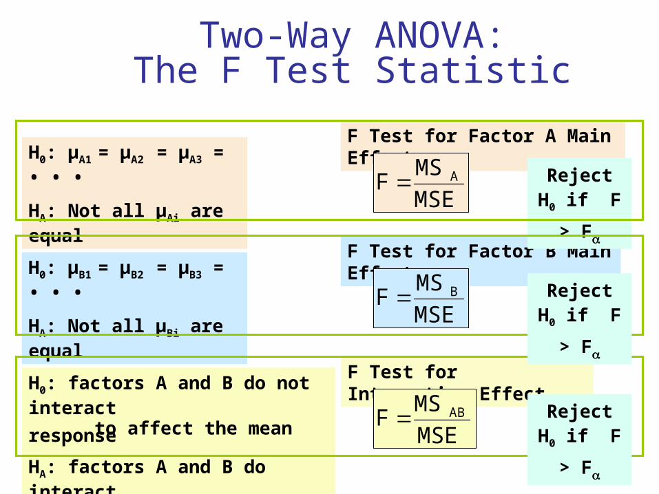
Two-Way ANOVA:The F Test Statistic

F Test for Factor B Main Effect

F Test for Interaction Effect

H0: μA1 = μA2 = μA3 = • • •

HA: Not all μAi are equal

H0: factors A and B do not interact to affect the mean response

HA: factors A and B do interact

F Test for Factor A Main Effect

H0: μB1 = μB2 = μB3 = • • •

HA: Not all μBi are equal

Reject H0

if F > FMSE

MSF A

MSE

MSF B

MSE

MSF AB

Reject H0

if F > F

Reject H0

if F > F

Two-Way ANOVASummary Table

Source ofVariation

Sum ofSquares

Degrees of Freedom

Mean Squares

FStatistic

Factor A SSA a – 1MSA

= SSA /(a – 1)

MSA

MSE

Factor B SSB b – 1MSB

= SSB /(b – 1)

MSB

MSE

AB(Interaction)

SSAB (a – 1)(b – 1)MSAB

= SSAB / [(a – 1)(b – 1)]

MSAB

MSE

Error SSE N – abMSE =

SSE/(N – ab)

Total SST N – 1

Features of Two-Way ANOVA F Test

• Degrees of freedom always add up

– N-1 = (N-ab) + (a-1) + (b-1) + (a-1)(b-1)

– Total = error + factor A + factor B + interaction

• The denominator of the F Test is always the same but the numerator is different

• The sums of squares always add up

– SST = SSE + SSA + SSB + SSAB

– Total = error + factor A + factor B + interaction

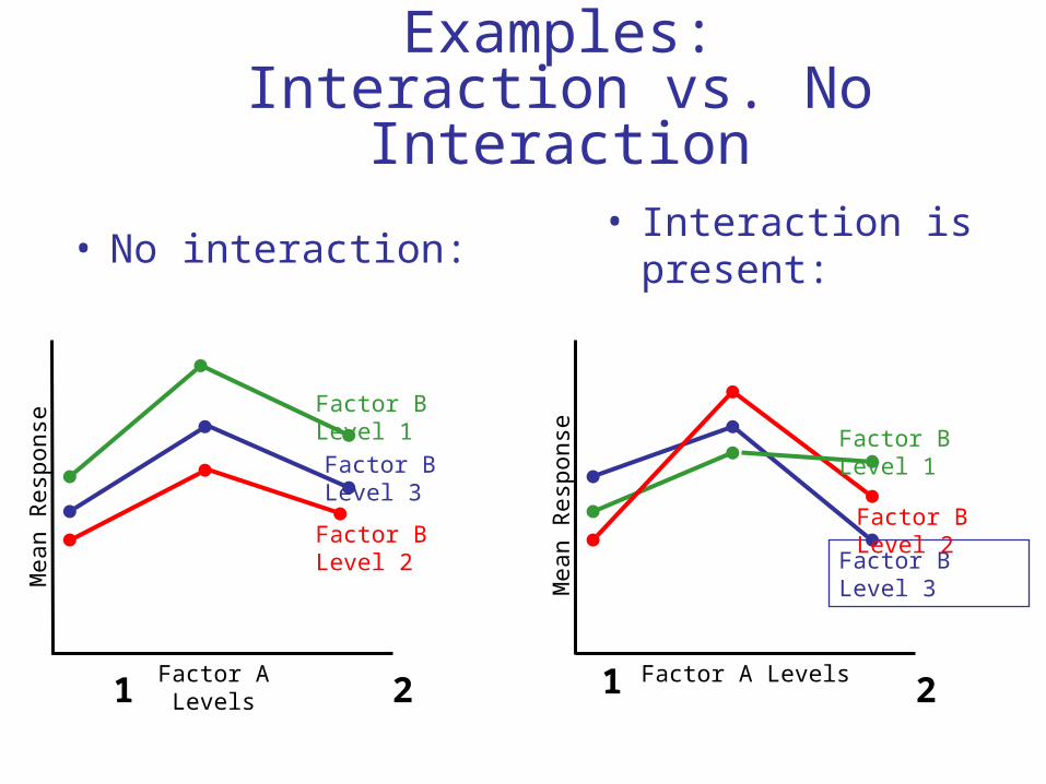
Examples:Interaction vs. No Interaction

• No interaction:

1 2

Factor B Level 1

Factor B Level 3

Factor B Level 2

Factor A Levels 1 2

Factor B Level 1

Factor B Level 3

Factor B Level 2

Factor A Levels

Mea

n R

espo

nse

Mea

n R

espo

nse

• Interaction is present:

Summary

• Described one-way analysis of variance– The logic of ANOVA– ANOVA assumptions– F test for difference in k means– The Tukey-Kramer procedure for multiple

comparisons

• Described two-way analysis of variance– Examined effects of multiple factors and interaction