Lecture 8a: Spurious Regression

1

Old Stuff

• The traditional statistical theory holds when we run regression

using (weakly or covariance) stationary variables.

• For example, when we regress one stationary series onto another

stationary series, the coefficient will be close to zero and

insignificant if the two series are independent.

• That is NOT the case when the two series are two independent

random walks, which are nonstationary

2

Spurious Regression

• The regression is spurious when we regress one random walk onto

another independent random walk. It is spurious because the

regression will most likely indicate a non-existing relationship:

1. The coefficient estimate will not converge toward zero (the

true value). Instead, in the limit the coefficient estimate will

follow a non-degenerate distribution

2. The t value most often is significant.

3. R2 is typically very high.

3

Simulation

# by construction y and x are two independent random walks

y = rep(0,n)

x = rep(0,n)

ey = rnorm(n)

ex = rnorm(n)

rhoy = 1

rhox = 1

for (i in 2:n) {

y[i] = rhoy*y[i-1] + ey[i]

x[i] = rhox*x[i-1] + ex[i]

}

4

Result of Spurious Regression

lm(formula = y ~ x)

Coefficients:

Estimate Std. Error t value Pr(>|t|)

(Intercept) -3.43193 0.31671 -10.836 < 2e-16 ***

x 0.31607 0.08013 3.944 0.000111 ***

The estimated coefficient of x is 0.31607, and is significant, despite

that the true coefficient is zero. This result mistakenly indicates that

y and x are related; actually they are independent of each other.

5

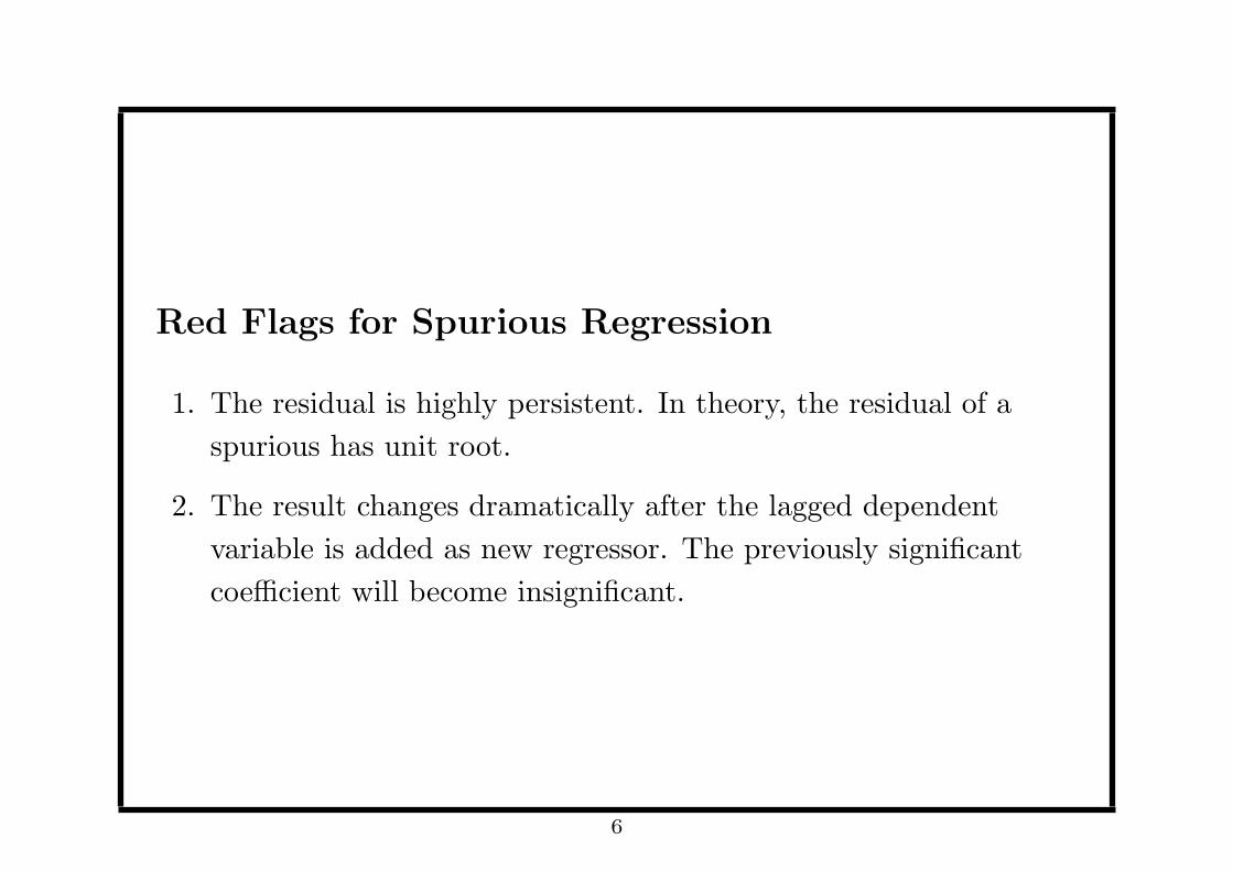
Red Flags for Spurious Regression

1. The residual is highly persistent. In theory, the residual of a

spurious has unit root.

2. The result changes dramatically after the lagged dependent

variable is added as new regressor. The previously significant

coefficient will become insignificant.

6

Lesson: always check the stationarity of the

residual. The regression is spurious if the residual

is nonstationary (cannot reject the null hypothesis

of the unit root test)

7

What causes the spurious regression?

Loosely speaking, because a nonstationary series contains

“stochastic” trend

1. For a random walk yt = yt−1 + et we can show its MA

representation is

yt = et + et−1 + et−2 + . . .

2. The stochastic trend et + et−1 + et−2 + . . . causes the series to

appear trending (locally).

3. Spurious regression happens when there are similar local trends.

8

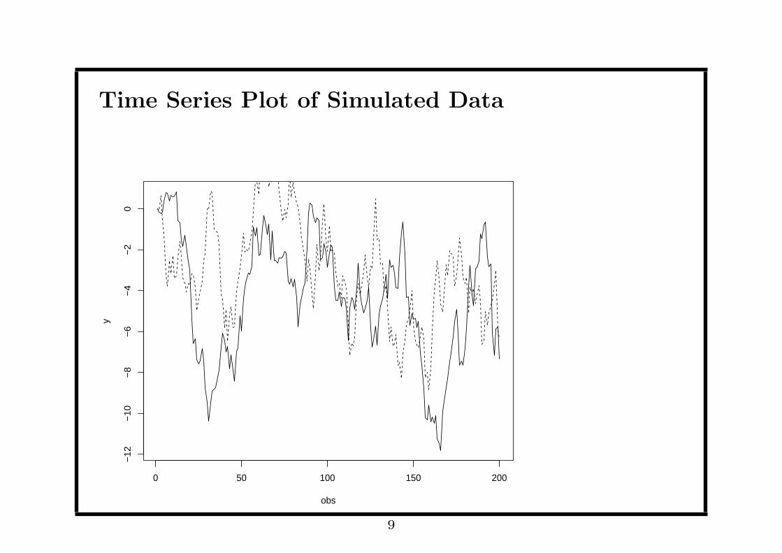
Time Series Plot of Simulated Data

0 50 100 150 200

−12

−10

−8

−6

−4

−2

0

obs

y

9

The solid line is y and dotted line is x. Sometimes their local trends

are similar, giving rise to the spurious regression.

10

Lesson: just because two series move together does

not mean they are related!

11

Lesson: use extra caution when you run regression

using nonstationary variables; be aware of the

possibility of spurious regression! Check whether

the residual is nonstationary.

12

Lecture 8b: Cointegration

13

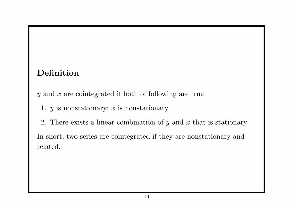
Definition

y and x are cointegrated if both of following are true

1. y is nonstationary; x is nonstationary

2. There exists a linear combination of y and x that is stationary

In short, two series are cointegrated if they are nonstationary and

related.

14

Economic Theory

Many economic theories imply cointegration. Two examples are

1. consumption = a+ b× income+ e

2. nominal interest rate =

inflation rate+ real interest rate

Exercise: can you think of another example?

15

OLS Estimator is Superconsistent

Unlike the spurious regression, when y and x are cointegrated,

regressing y onto x makes super sense. “Super” because the

coefficient estimate will converge to the true value (which is nonzero)

super fast (at rate of T−1 instead of T−1/2).

16

Simulation

# y and x are nonstationary but related (cointegrated)

y = rep(0,n)

x = rep(0,n)

ey = rnorm(n)

ex = rnorm(n)

beta = 4

rhox = 1

for (i in 2:n) {

x[i] = rhox*x[i-1] + ex[i]

y[i] = beta*x[i] + ey[i]

}

17

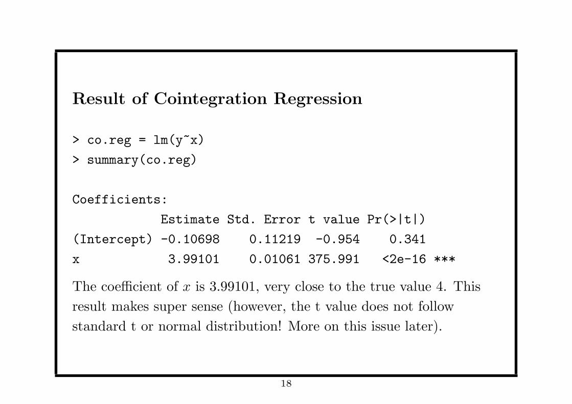
Result of Cointegration Regression

> co.reg = lm(y~x)

> summary(co.reg)

Coefficients:

Estimate Std. Error t value Pr(>|t|)

(Intercept) -0.10698 0.11219 -0.954 0.341

x 3.99101 0.01061 375.991 <2e-16 ***

The coefficient of x is 3.99101, very close to the true value 4. This

result makes super sense (however, the t value does not follow

standard t or normal distribution! More on this issue later).

18

Residual is stationary for cointegrated series

> co.res = co.reg$res

> adf.test(co.res, k = 1)

Augmented Dickey-Fuller Test

data: co.res

Dickey-Fuller = -10.4398, Lag order = 1, p-value = 0.01

alternative hypothesis: stationary

The p-value is less than 0.05, so rejects the null hypothesis of unit

root (rigorously speaking, the p-value is wrong here because it is

based on the Dickey-Fuller distribution. More on this issue later).

19

Engle-Granger Test for Cointegration

The Engle-Granger cointegration test (1987, Econometrica) is

essentially the unit root test applied to the residual of cointegration

regression

1. The series are cointegrated if the residual has no unit root

2. The series are not cointegrated (and the regression is spurious) if

the residual has unit root

The null hypothesis is that the series are NOT cointegrated.

20

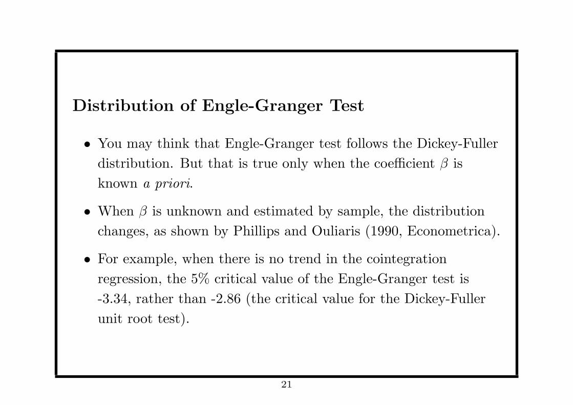
Distribution of Engle-Granger Test

• You may think that Engle-Granger test follows the Dickey-Fuller

distribution. But that is true only when the coefficient β is

known a priori.

• When β is unknown and estimated by sample, the distribution

changes, as shown by Phillips and Ouliaris (1990, Econometrica).

• For example, when there is no trend in the cointegration

regression, the 5% critical value of the Engle-Granger test is

-3.34, rather than -2.86 (the critical value for the Dickey-Fuller

unit root test).

21

Simulation

Step 1: we need to generate y and x under the null hypothesis,

which is that they are not cointegrated

Step 2: then we regress y onto x, and save the residual

Step 3: we regress the differenced residual onto its first lag. The

t value of the first lagged residual is the Engle-Granger test

Step 4: we repeat Steps 1,2,3 many times. The 5% percentile of

the distribution of the t values is the 5% critical value for the

Engle-Granger test

22

Lesson: make sure you are using the correct critical

values when running the cointegration test.

23

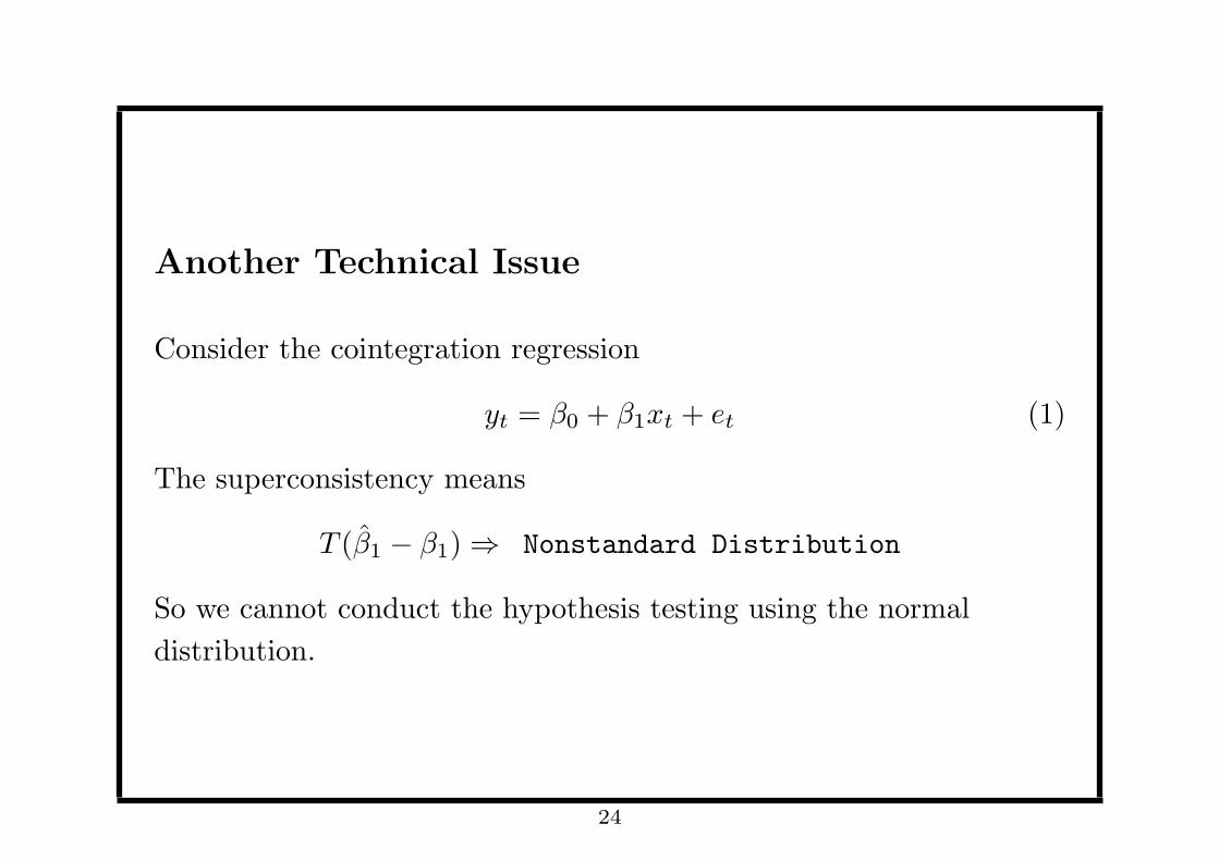
Another Technical Issue

Consider the cointegration regression

yt = β0 + β1xt + et (1)

The superconsistency means

T (β1 − β1) ⇒ Nonstandard Distribution

So we cannot conduct the hypothesis testing using the normal

distribution.

24

Example

For the consumption-income relationship, we may test the null

hypothesis that the marginal propensity to consume is unity, ie.,

H0 : β1 = 1

We can construct the t test as usual. However, we cannot compare it

to the critical values of t distribution or normal distribution.

25

Dynamic OLS (DOLS) Estimator

Stock and Watson (1993, Econometrica) suggest adding the leads and

lags of ∆xt as new regressors

yt = β0 + β1xt +

p∑i=−p

ci∆xt−i + et (2)

Now β1 is called dynamic OLS estimator, and it is asymptotically

normally distributed.

26

Lesson: use DOLS estimator so that the normal

distribution can be used in hypothesis testing

27

Lecture 8c: Vector Error Correction Model

28

Big Picture of Multivariate Model

1. We can apply VAR if series are stationary

2. We can apply VAR to differenced series if they are nonstationary

and not cointegrated

3. We need to apply vector error correction model if series are

nonstationary and cointegrated

29

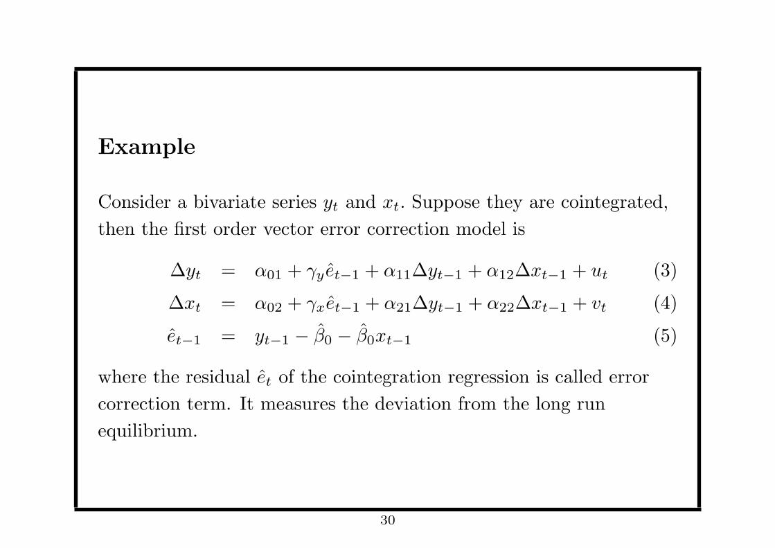
Example

Consider a bivariate series yt and xt. Suppose they are cointegrated,

then the first order vector error correction model is

∆yt = α01 + γy et−1 + α11∆yt−1 + α12∆xt−1 + ut (3)

∆xt = α02 + γxet−1 + α21∆yt−1 + α22∆xt−1 + vt (4)

et−1 = yt−1 − β0 − β0xt−1 (5)

where the residual et of the cointegration regression is called error

correction term. It measures the deviation from the long run

equilibrium.

30

Intuition

1. Note that the residual et is stationary when the series are

cointegrated. So it makes sense to use it to explain the stationary

∆yt and ∆xt.

2. There will be omitted variable bias if we apply VAR to

differenced series when they are cointegrated; the omitted

variable is et−1

3. It is called error correction model because it shows how variable

adjusts to the deviation from the equilibrium (the error

correction term)

4. The speed of error correction is captured by γy and γx.

31

Engle-Granger Two Step Procedure

Step 1: Obtain the error correction term, or the residual of the

cointegration regression (5).

Step 2: Estimate (3) and (4) using OLS.

In the second step, we can treat the estimated β0 and β1 as the true

values since they are super-consistent.

32

Hypothesis Testing

1. All the variables in the error correction models are stationary if

the series are cointegrated. So the t test and f test follow the

standard distributions.

2. In particular, we can apply the standard test for Granger

Causality:

H0 : α12 = 0

H0 : α21 = 0

33

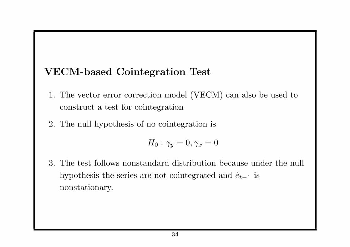
VECM-based Cointegration Test

1. The vector error correction model (VECM) can also be used to

construct a test for cointegration

2. The null hypothesis of no cointegration is

H0 : γy = 0, γx = 0

3. The test follows nonstandard distribution because under the null

hypothesis the series are not cointegrated and et−1 is

nonstationary.

34

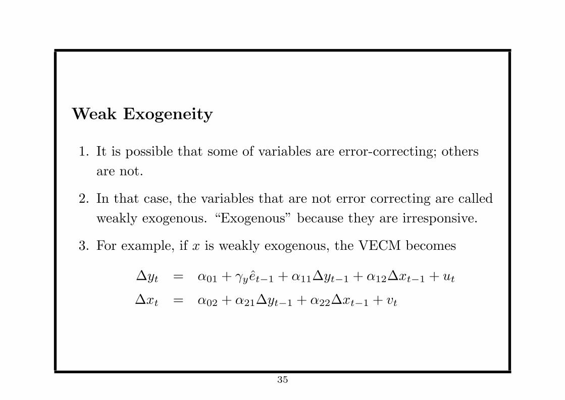
Weak Exogeneity

1. It is possible that some of variables are error-correcting; others

are not.

2. In that case, the variables that are not error correcting are called

weakly exogenous. “Exogenous” because they are irresponsive.

3. For example, if x is weakly exogenous, the VECM becomes

∆yt = α01 + γy et−1 + α11∆yt−1 + α12∆xt−1 + ut

∆xt = α02 + α21∆yt−1 + α22∆xt−1 + vt

35

Lecture 8d: Empirical Example

36

Data

• We are interested in the relationship between the federal fund

rate (sr), 3-month treasury bill rate (mr) and 10-year treasury

bond rate (lr)

• The monthly data from Jan 1982 to Jan 2014 are downloaded

from Fred data.

37

Plot

Monthly Interest Rates

Time

Inte

rest

Rat

es

1985 1990 1995 2000 2005 2010 2015

24

68

1012

14

38

We see overall the three series tend to move together (sr and mr are

particularly close). Nevertheless we are not sure the co-movement (or

similar local trends) indicates a spurious regression or a cointegration.

39

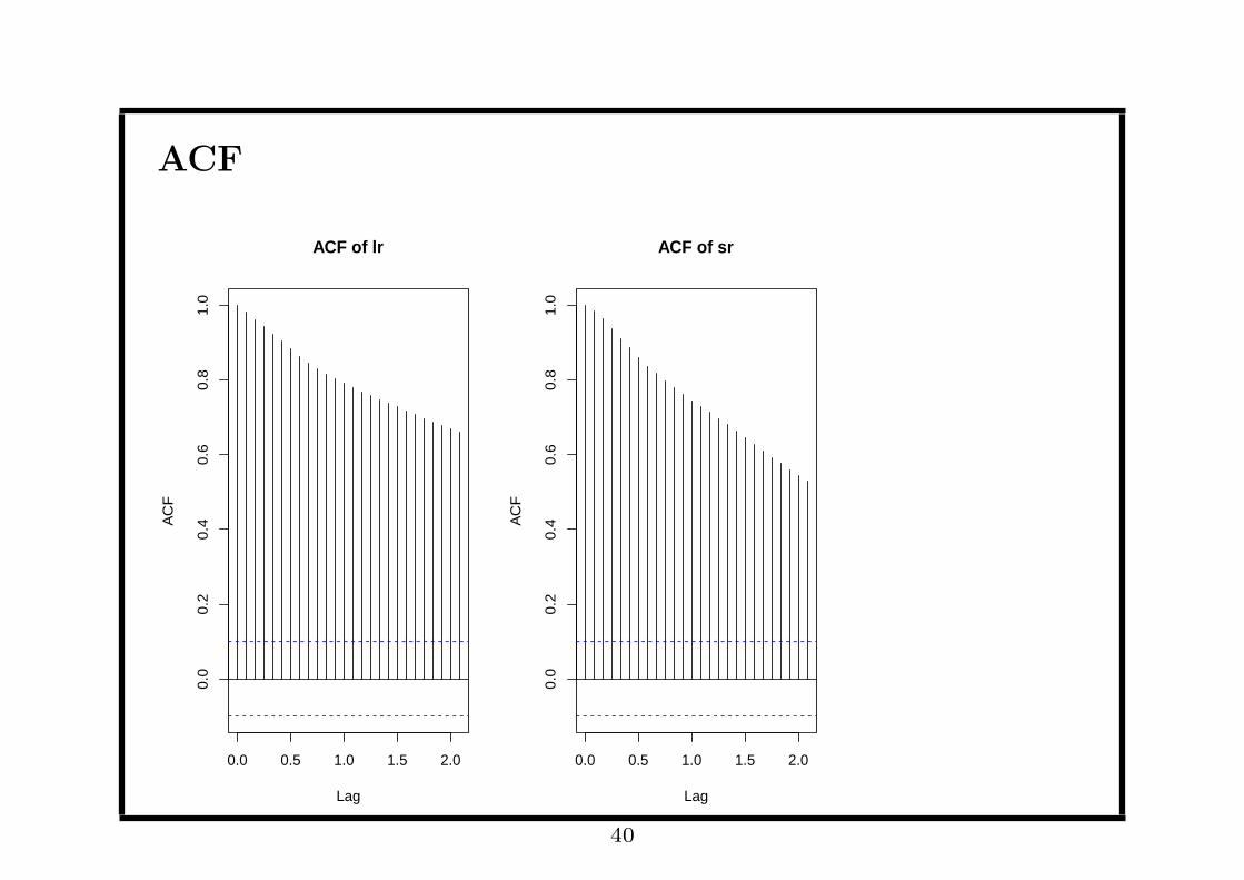
ACF

0.0 0.5 1.0 1.5 2.0

0.0

0.2

0.4

0.6

0.8

1.0

Lag

AC

F

ACF of lr

0.0 0.5 1.0 1.5 2.0

0.0

0.2

0.4

0.6

0.8

1.0

Lag

AC

F

ACF of sr

40

lr and sr seem nonstationary as their ACF decays very slowly.

41

Unit Root Test

ob = length(lr)

lr.1 = c(NA, lr[1:ob-1]) # first lag

dlr = lr - lr.1 # difference

summary(lm(dlr~lr.1))

Coefficients:

Estimate Std. Error t value Pr(>|t|)

(Intercept) 0.057562 0.034181 1.684 0.09300 .

lr.1 -0.013961 0.004939 -2.827 0.00495 **

The adf test with zero lag is -2.827, greater than the 5% critical value

-2.86. So the null hypothesis of unit root cannot be rejected for lr.

42

Cointegration Regression

> co.reg = lm(lr~sr)

> summary(co.reg)

Coefficients:

Estimate Std. Error t value Pr(>|t|)

(Intercept) 2.51249 0.10031 25.05 <2e-16 ***

sr 0.80281 0.01749 45.89 <2e-16 ***

So β0 = 2.51249, β1 = 0.80281. Those are super-consistent estimates.

43

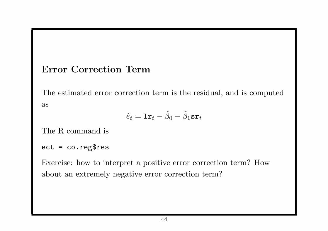
Error Correction Term

The estimated error correction term is the residual, and is computed

as

et = lrt − β0 − β1srt

The R command is

ect = co.reg$res

Exercise: how to interpret a positive error correction term? How

about an extremely negative error correction term?

44

Exercise: how to obtain the DOLS estimator of β0

and β1?

45

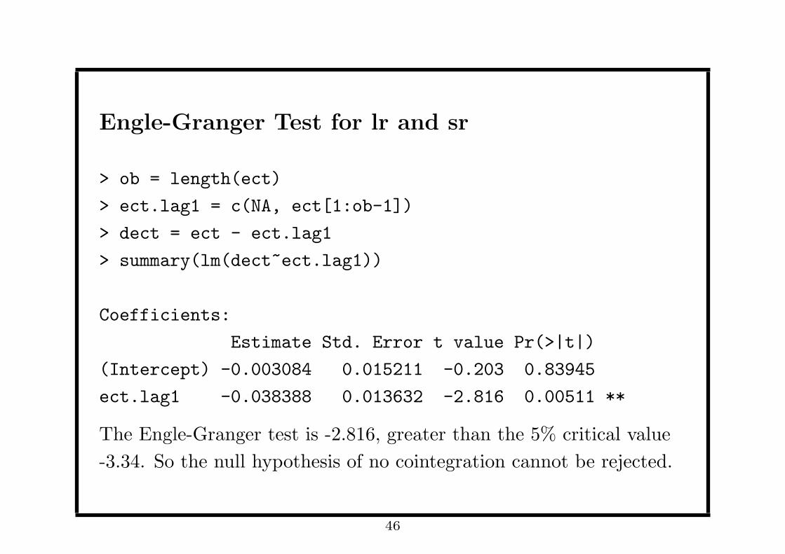
Engle-Granger Test for lr and sr

> ob = length(ect)

> ect.lag1 = c(NA, ect[1:ob-1])

> dect = ect - ect.lag1

> summary(lm(dect~ect.lag1))

Coefficients:

Estimate Std. Error t value Pr(>|t|)

(Intercept) -0.003084 0.015211 -0.203 0.83945

ect.lag1 -0.038388 0.013632 -2.816 0.00511 **

The Engle-Granger test is -2.816, greater than the 5% critical value

-3.34. So the null hypothesis of no cointegration cannot be rejected.

46

Remark

This result is not surprising. Basically it says that the relation

between the federal fund rate and 10 year rate is very weak (not as

strong as cointegration). Given no cointegration, the appropriate

multivariate model is VAR in difference.

47

VAR in difference for lr and sr

lm(formula = dsr ~ dlr.1 + dsr.1)

Estimate Std. Error t value Pr(>|t|)

(Intercept) -0.02046 0.01256 -1.629 0.104110

dlr.1 0.15746 0.04715 3.340 0.000921 ***

dsr.1 0.38339 0.04555 8.417 7.99e-16 ***

lm(formula = dlr ~ dlr.1 + dsr.1)

Estimate Std. Error t value Pr(>|t|)

(Intercept) -0.01918 0.01351 -1.420 0.156

dlr.1 0.32944 0.05072 6.495 2.61e-10 ***

dsr.1 0.02825 0.04901 0.577 0.565

48

It seems that sr does not Granger cause lr. Does this result make

sense?

49

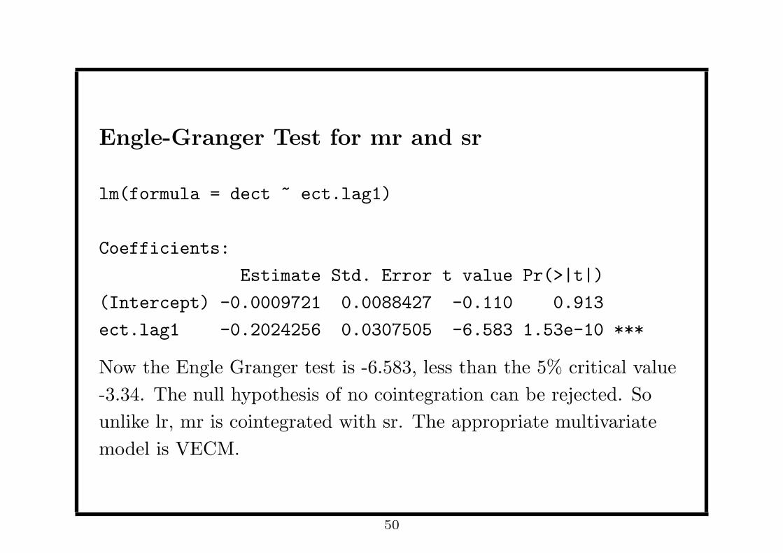
Engle-Granger Test for mr and sr

lm(formula = dect ~ ect.lag1)

Coefficients:

Estimate Std. Error t value Pr(>|t|)

(Intercept) -0.0009721 0.0088427 -0.110 0.913

ect.lag1 -0.2024256 0.0307505 -6.583 1.53e-10 ***

Now the Engle Granger test is -6.583, less than the 5% critical value

-3.34. The null hypothesis of no cointegration can be rejected. So

unlike lr, mr is cointegrated with sr. The appropriate multivariate

model is VECM.

50

ECM for sr

lm(formula = dsr ~ ect.1 + dmr.1 + dsr.1)

Coefficients:

Estimate Std. Error t value Pr(>|t|)

(Intercept) -0.02478 0.01208 -2.050 0.041 *

ect.1 0.25031 0.04626 5.411 1.11e-07 ***

dmr.1 0.08862 0.07337 1.208 0.228

dsr.1 0.31101 0.06649 4.677 4.05e-06 ***

So sr is error correcting (t-value for error correction term is 5.411). It

seems that mr does not Granger cause sr (t-value for ∆mrt−1 is 1.208)

51

ECM for mr

lm(formula = dmr ~ ect.1 + dmr.1 + dsr.1)

Coefficients:

Estimate Std. Error t value Pr(>|t|)

(Intercept) -0.01969 0.01251 -1.574 0.1162

ect.1 -0.01457 0.04788 -0.304 0.7610

dmr.1 0.17723 0.07594 2.334 0.0201 *

dsr.1 0.28467 0.06881 4.137 4.34e-05 ***

mr is weakly exogenous or not error correcting (t-value for error

correction term is -0.304). It seems that sr Granger causes mr

(t-value for ∆srt−1 is 4.137)

52