lecture 8: integrating learning and planning - ucl · this lecture: learnmodeldirectly ... a model...
TRANSCRIPT

Lecture 8: Integrating Learning and Planning
Lecture 8: Integrating Learning and Planning
David Silver

Lecture 8: Integrating Learning and Planning
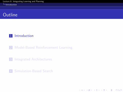
Outline
1 Introduction
2 Model-Based Reinforcement Learning
3 Integrated Architectures
4 Simulation-Based Search
Lecture 8: Integrating Learning and Planning
Introduction
Outline
1 Introduction
2 Model-Based Reinforcement Learning
3 Integrated Architectures
4 Simulation-Based Search

Lecture 8: Integrating Learning and Planning
Introduction
Model-Based Reinforcement Learning
Last lecture: learn policy directly from experience
Previous lectures: learn value function directly from experience
This lecture: learn model directly from experience
and use planning to construct a value function or policy
Integrate learning and planning into a single architecture

Lecture 8: Integrating Learning and Planning
Introduction
Model-Based and Model-Free RL
Model-Free RL
No modelLearn value function (and/or policy) from experience
Model-Based RL
Learn a model from experiencePlan value function (and/or policy) from model

Lecture 8: Integrating Learning and Planning
Introduction
Model-Based and Model-Free RL
Model-Free RL
No modelLearn value function (and/or policy) from experience
Model-Based RL
Learn a model from experiencePlan value function (and/or policy) from model

Lecture 8: Integrating Learning and Planning
Introduction
Model-Free RL
state
reward
action
At
Rt
St

Lecture 8: Integrating Learning and Planning
Introduction
Model-Based RL
state
reward
action
At
Rt
St

Lecture 8: Integrating Learning and Planning
Model-Based Reinforcement Learning
Outline
1 Introduction
2 Model-Based Reinforcement Learning
3 Integrated Architectures
4 Simulation-Based Search

Lecture 8: Integrating Learning and Planning
Model-Based Reinforcement Learning
Model-Based RL

Lecture 8: Integrating Learning and Planning
Model-Based Reinforcement Learning
Advantages of Model-Based RL
Advantages:
Can efficiently learn model by supervised learning methods
Can reason about model uncertainty
Disadvantages:
First learn a model, then construct a value function⇒ two sources of approximation error

Lecture 8: Integrating Learning and Planning
Model-Based Reinforcement Learning
Learning a Model
What is a Model?
A modelM is a representation of an MDP 〈S,A,P,R〉,parametrized by η
We will assume state space S and action space A are known
So a model M = 〈Pη,Rη〉 represents state transitionsPη ≈ P and rewards Rη ≈ R
St+1 ∼ Pη(St+1 | St ,At)
Rt+1 = Rη(Rt+1 | St ,At)
Typically assume conditional independence between statetransitions and rewards
P [St+1,Rt+1 | St ,At ] = P [St+1 | St ,At ]P [Rt+1 | St ,At ]

Lecture 8: Integrating Learning and Planning
Model-Based Reinforcement Learning
Learning a Model
Model Learning
Goal: estimate modelMη from experience {S1,A1,R2, ...,ST}This is a supervised learning problem
S1,A1 → R2, S2
S2,A2 → R3, S3
...
ST−1,AT−1 → RT ,ST
Learning s, a→ r is a regression problem
Learning s, a→ s ′ is a density estimation problem
Pick loss function, e.g. mean-squared error, KL divergence, ...
Find parameters η that minimise empirical loss

Lecture 8: Integrating Learning and Planning
Model-Based Reinforcement Learning
Learning a Model
Examples of Models
Table Lookup Model
Linear Expectation Model
Linear Gaussian Model
Gaussian Process Model
Deep Belief Network Model
...

Lecture 8: Integrating Learning and Planning
Model-Based Reinforcement Learning
Learning a Model
Table Lookup Model
Model is an explicit MDP, P̂, R̂Count visits N(s, a) to each state action pair
P̂as,s′ =
1
N(s, a)
T∑t=1
1(St ,At , St+1 = s, a, s ′)
R̂as =
1
N(s, a)
T∑t=1
1(St ,At = s, a)Rt
Alternatively
At each time-step t, record experience tuple〈St ,At ,Rt+1,St+1〉To sample model, randomly pick tuple matching 〈s, a, ·, ·〉

Lecture 8: Integrating Learning and Planning
Model-Based Reinforcement Learning
Learning a Model
AB Example
Two states A,B; no discounting; 8 episodes of experience
A, 0, B, 0!B, 1!B, 1!B, 1!B, 1!B, 1!B, 1!B, 0!
We have constructed a table lookup model from the experience

Lecture 8: Integrating Learning and Planning
Model-Based Reinforcement Learning
Planning with a Model
Planning with a Model
Given a model Mη = 〈Pη,Rη〉Solve the MDP 〈S,A,Pη,Rη〉Using favourite planning algorithm
Value iterationPolicy iterationTree search...

Lecture 8: Integrating Learning and Planning
Model-Based Reinforcement Learning
Planning with a Model
Sample-Based Planning
A simple but powerful approach to planning
Use the model only to generate samples
Sample experience from model
St+1 ∼ Pη(St+1 | St ,At)
Rt+1 = Rη(Rt+1 | St ,At)
Apply model-free RL to samples, e.g.:
Monte-Carlo controlSarsaQ-learning
Sample-based planning methods are often more efficient
Lecture 8: Integrating Learning and Planning
Model-Based Reinforcement Learning
Planning with a Model
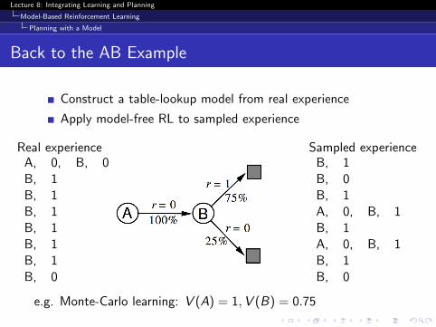
Back to the AB Example
Construct a table-lookup model from real experience
Apply model-free RL to sampled experience
Real experienceA, 0, B, 0B, 1B, 1B, 1B, 1B, 1B, 1B, 0
Sampled experienceB, 1B, 0B, 1A, 0, B, 1B, 1A, 0, B, 1B, 1B, 0
e.g. Monte-Carlo learning: V (A) = 1,V (B) = 0.75
Lecture 8: Integrating Learning and Planning
Model-Based Reinforcement Learning
Planning with a Model
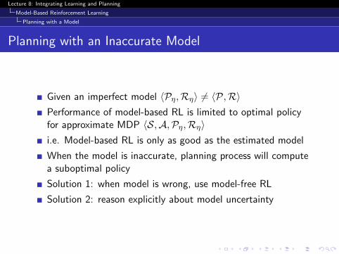
Planning with an Inaccurate Model
Given an imperfect model 〈Pη,Rη〉 6= 〈P,R〉Performance of model-based RL is limited to optimal policyfor approximate MDP 〈S,A,Pη,Rη〉i.e. Model-based RL is only as good as the estimated model
When the model is inaccurate, planning process will computea suboptimal policy
Solution 1: when model is wrong, use model-free RL
Solution 2: reason explicitly about model uncertainty

Lecture 8: Integrating Learning and Planning
Integrated Architectures
Outline
1 Introduction
2 Model-Based Reinforcement Learning
3 Integrated Architectures
4 Simulation-Based Search

Lecture 8: Integrating Learning and Planning
Integrated Architectures
Dyna
Real and Simulated Experience
We consider two sources of experience
Real experience Sampled from environment (true MDP)
S ′ ∼ Pas,s′
R = Ras
Simulated experience Sampled from model (approximate MDP)
S ′ ∼ Pη(S ′ | S ,A)
R = Rη(R | S ,A)
Lecture 8: Integrating Learning and Planning
Integrated Architectures
Dyna
Integrating Learning and Planning
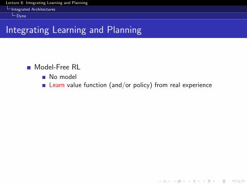
Model-Free RL
No modelLearn value function (and/or policy) from real experience
Model-Based RL (using Sample-Based Planning)
Learn a model from real experiencePlan value function (and/or policy) from simulated experience
Dyna
Learn a model from real experienceLearn and plan value function (and/or policy) from real andsimulated experience

Lecture 8: Integrating Learning and Planning
Integrated Architectures
Dyna
Integrating Learning and Planning
Model-Free RL
No modelLearn value function (and/or policy) from real experience
Model-Based RL (using Sample-Based Planning)
Learn a model from real experiencePlan value function (and/or policy) from simulated experience
Dyna
Learn a model from real experienceLearn and plan value function (and/or policy) from real andsimulated experience

Lecture 8: Integrating Learning and Planning
Integrated Architectures
Dyna
Dyna Architecture

Lecture 8: Integrating Learning and Planning
Integrated Architectures
Dyna
Dyna-Q Algorithm

Lecture 8: Integrating Learning and Planning
Integrated Architectures
Dyna
Dyna-Q on a Simple Maze
Lecture 8: Integrating Learning and Planning
Integrated Architectures
Dyna
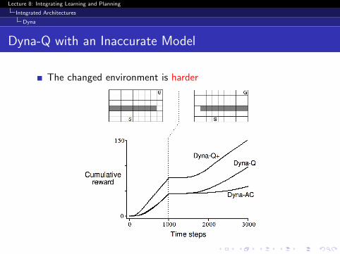
Dyna-Q with an Inaccurate Model
The changed environment is harder

Lecture 8: Integrating Learning and Planning
Integrated Architectures
Dyna
Dyna-Q with an Inaccurate Model (2)
The changed environment is easier

Lecture 8: Integrating Learning and Planning
Simulation-Based Search
Outline
1 Introduction
2 Model-Based Reinforcement Learning
3 Integrated Architectures
4 Simulation-Based Search

Lecture 8: Integrating Learning and Planning
Simulation-Based Search
Forward Search
Forward search algorithms select the best action by lookahead
They build a search tree with the current state st at the root
Using a model of the MDP to look ahead
T! T! T! T!T!
T! T! T! T! T!
st
T! T!
T! T!
T!T! T!
T! T!T!
No need to solve whole MDP, just sub-MDP starting from now

Lecture 8: Integrating Learning and Planning
Simulation-Based Search
Simulation-Based Search
Forward search paradigm using sample-based planning
Simulate episodes of experience from now with the model
Apply model-free RL to simulated episodes
T! T! T! T!T!
T! T! T! T! T!
st
T! T!
T! T!
T!T! T!
T! T!T!
Lecture 8: Integrating Learning and Planning
Simulation-Based Search
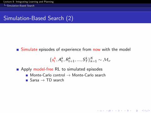
Simulation-Based Search (2)
Simulate episodes of experience from now with the model
{skt ,Akt ,R
kt+1, ...,S
kT}Kk=1 ∼Mν
Apply model-free RL to simulated episodes
Monte-Carlo control → Monte-Carlo searchSarsa → TD search

Lecture 8: Integrating Learning and Planning
Simulation-Based Search
Monte-Carlo Search
Simple Monte-Carlo Search
Given a model Mν and a simulation policy π
For each action a ∈ ASimulate K episodes from current (real) state st
{st , a,Rkt+1,S
kt+1,A
kt+1, ...,S
kT}Kk=1 ∼Mν , π
Evaluate actions by mean return (Monte-Carlo evaluation)
Q(st , a) =1
K
K∑k=1
GtP→ qπ(st , a)
Select current (real) action with maximum value
at = argmaxa∈A
Q(st , a)

Lecture 8: Integrating Learning and Planning
Simulation-Based Search
Monte-Carlo Search
Monte-Carlo Tree Search (Evaluation)
Given a model Mν
Simulate K episodes from current state st using currentsimulation policy π
{st ,Akt ,R
kt+1,S
kt+1, ...,S
kT}Kk=1 ∼Mν , π
Build a search tree containing visited states and actions
Evaluate states Q(s, a) by mean return of episodes from s, a
Q(s, a) =1
N(s, a)
K∑k=1
T∑u=t
1(Su,Au = s, a)GuP→ qπ(s, a)
After search is finished, select current (real) action withmaximum value in search tree
at = argmaxa∈A
Q(st , a)

Lecture 8: Integrating Learning and Planning
Simulation-Based Search
Monte-Carlo Search
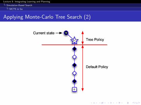
Monte-Carlo Tree Search (Simulation)
In MCTS, the simulation policy π improves
Each simulation consists of two phases (in-tree, out-of-tree)
Tree policy (improves): pick actions to maximise Q(S ,A)Default policy (fixed): pick actions randomly
Repeat (each simulation)
Evaluate states Q(S ,A) by Monte-Carlo evaluationImprove tree policy, e.g. by ε− greedy(Q)
Monte-Carlo control applied to simulated experience
Converges on the optimal search tree, Q(S ,A)→ q∗(S ,A)

Lecture 8: Integrating Learning and Planning
Simulation-Based Search
MCTS in Go
Case Study: the Game of Go
The ancient oriental game ofGo is 2500 years old
Considered to be the hardestclassic board game
Considered a grandchallenge task for AI(John McCarthy)
Traditional game-tree searchhas failed in Go

Lecture 8: Integrating Learning and Planning
Simulation-Based Search
MCTS in Go
Rules of Go
Usually played on 19x19, also 13x13 or 9x9 board
Simple rules, complex strategy
Black and white place down stones alternately
Surrounded stones are captured and removed
The player with more territory wins the game

Lecture 8: Integrating Learning and Planning
Simulation-Based Search
MCTS in Go
Position Evaluation in Go
How good is a position s?
Reward function (undiscounted):
Rt = 0 for all non-terminal steps t < T
RT =
{1 if Black wins0 if White wins
Policy π = 〈πB , πW 〉 selects moves for both players
Value function (how good is position s):
vπ(s) = Eπ [RT | S = s] = P [Black wins | S = s]
v∗(s) = maxπB
minπW
vπ(s)

Lecture 8: Integrating Learning and Planning
Simulation-Based Search
MCTS in Go
Monte-Carlo Evaluation in Go
Current position s
Simulation
1 1 0 0 Outcomes
V(s) = 2/4 = 0.5

Lecture 8: Integrating Learning and Planning
Simulation-Based Search
MCTS in Go
Applying Monte-Carlo Tree Search (1)
Lecture 8: Integrating Learning and Planning
Simulation-Based Search
MCTS in Go
Applying Monte-Carlo Tree Search (2)

Lecture 8: Integrating Learning and Planning
Simulation-Based Search
MCTS in Go
Applying Monte-Carlo Tree Search (3)

Lecture 8: Integrating Learning and Planning
Simulation-Based Search
MCTS in Go
Applying Monte-Carlo Tree Search (4)

Lecture 8: Integrating Learning and Planning
Simulation-Based Search
MCTS in Go
Applying Monte-Carlo Tree Search (5)
Lecture 8: Integrating Learning and Planning
Simulation-Based Search
MCTS in Go
Advantages of MC Tree Search
Highly selective best-first search
Evaluates states dynamically (unlike e.g. DP)
Uses sampling to break curse of dimensionality
Works for “black-box” models (only requires samples)
Computationally efficient, anytime, parallelisable

Lecture 8: Integrating Learning and Planning
Simulation-Based Search
MCTS in Go
Example: MC Tree Search in Computer Go
Jul 06 Jan 07 Jul 07 Jan 08 Jul 08 Jan 09 Jul 09 Jan 10 Jul 10 Jan 11
MoGo
MoGo
MoGoCrazyStone
CrazyStone
Fuego
Zen
Zen
Zen
Zen
Erica
GnuGo*
GnuGo*
ManyFaces*
ManyFaces
ManyFaces
ManyFaces
ManyFaces
ManyFaces
ManyFaces
Aya*
Aya*
Aya
Aya
Aya
Aya
Indigo
10 kyu
9 kyu
8 kyu
7 kyu
6 kyu
5 kyu
4 kyu
3 kyu
2 kyu
1 kyu
1 dan
2 dan
3 dan
4 dan
5 dan
Foo
1

Lecture 8: Integrating Learning and Planning
Simulation-Based Search
Temporal-Difference Search
Temporal-Difference Search
Simulation-based search
Using TD instead of MC (bootstrapping)
MC tree search applies MC control to sub-MDP from now
TD search applies Sarsa to sub-MDP from now

Lecture 8: Integrating Learning and Planning
Simulation-Based Search
Temporal-Difference Search
MC vs. TD search
For model-free reinforcement learning, bootstrapping is helpful
TD learning reduces variance but increases biasTD learning is usually more efficient than MCTD(λ) can be much more efficient than MC
For simulation-based search, bootstrapping is also helpful
TD search reduces variance but increases biasTD search is usually more efficient than MC searchTD(λ) search can be much more efficient than MC search

Lecture 8: Integrating Learning and Planning
Simulation-Based Search
Temporal-Difference Search
TD Search
Simulate episodes from the current (real) state st
Estimate action-value function Q(s, a)
For each step of simulation, update action-values by Sarsa
∆Q(S ,A) = α(R + γQ(S ′,A′)− Q(S ,A))
Select actions based on action-values Q(s, a)
e.g. ε-greedy
May also use function approximation for Q

Lecture 8: Integrating Learning and Planning
Simulation-Based Search
Temporal-Difference Search
Dyna-2
In Dyna-2, the agent stores two sets of feature weights
Long-term memoryShort-term (working) memory
Long-term memory is updated from real experienceusing TD learning
General domain knowledge that applies to any episode
Short-term memory is updated from simulated experienceusing TD search
Specific local knowledge about the current situation
Over value function is sum of long and short-term memories

Lecture 8: Integrating Learning and Planning
Simulation-Based Search
Temporal-Difference Search
Results of TD search in Go

Lecture 8: Integrating Learning and Planning
Simulation-Based Search
Temporal-Difference Search
Questions?