LECTURE 7 Monetary Policy at the Zero Lower Bound:

Expectations Effects

October 3, 2018

Economics 210c/236a Christina Romer Fall 2018 David Romer

I. OVERVIEW

Cases of Countries Hitting the Zero Lower Bound

• US and UK in the 1930s.

• Japan starting in the late 1990s.

• US, Europe, and Japan starting in 2008.

Papers for Today

• Temin and Wigmore (U.S. in the 1930s)

• Eggertsson and Pugsley (U.S. in 1937)

• Wieland (Japan, mainly in the 1990s and 2000s)

How can monetary policy matter at the zero lower bound?

• Expectations effects.

• Expectations of prices, growth, future interest rates.

• Quantitative easing and portfolio balance effects.

• Others?

• Special case of the exchange rate.

II. TEMIN AND WIGMORE, “THE END OF ONE BIG DEFLATION”

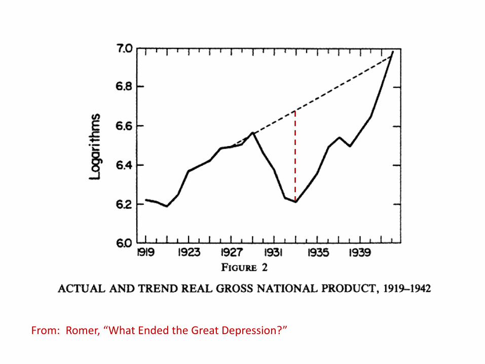
From: Romer, “What Ended the Great Depression?”

Nominal Interest Rate (3-6 mo. Treasury Notes)

0

1

2

3

4

5

6

Jan-

29

Jul-2

9

Jan-

30

Jul-3

0

Jan-

31

Jul-3

1

Jan-

32

Jul-3

2

Jan-

33

Jul-3

3

Jan-

34

Jul-3

4

Jan-

35

Jul-3

5

Per

cent

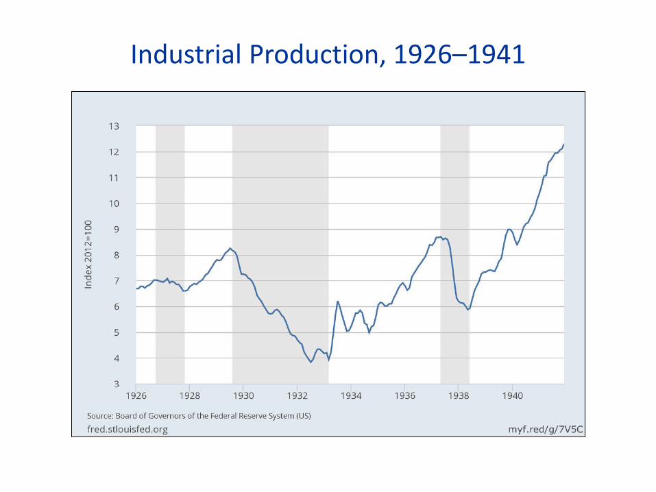
Industrial Production

1929

-01

1929

-07

1930

-01

1930

-07

1931

-01

1931

-07

1932

-01

1932

-07

1933

-01

1933

-07

1934

-01

1934

-07

1935

-01

1935

-07

1936

-01

1936

-07

1937

-01

1937

-07

1.0

1.2

1.4

1.6

1.8

2.0

2.2

2.4In

dust

rial P

rodu

ctio

n (L

ogar

ithm

s)

What is a regime shift?

• A dramatic change in the policy framework.

• Leads agents to expect long-lasting changes in policy.

Roosevelt’s Regime Shift

• Hoover was committed to the gold standard, monetary inaction, and fiscal orthodoxy.

• Roosevelt devalued in April 1933. Temin and Wigmore believe devaluation was the key sign of the regime shift.

• Followed up with fiscal and monetary expansion.

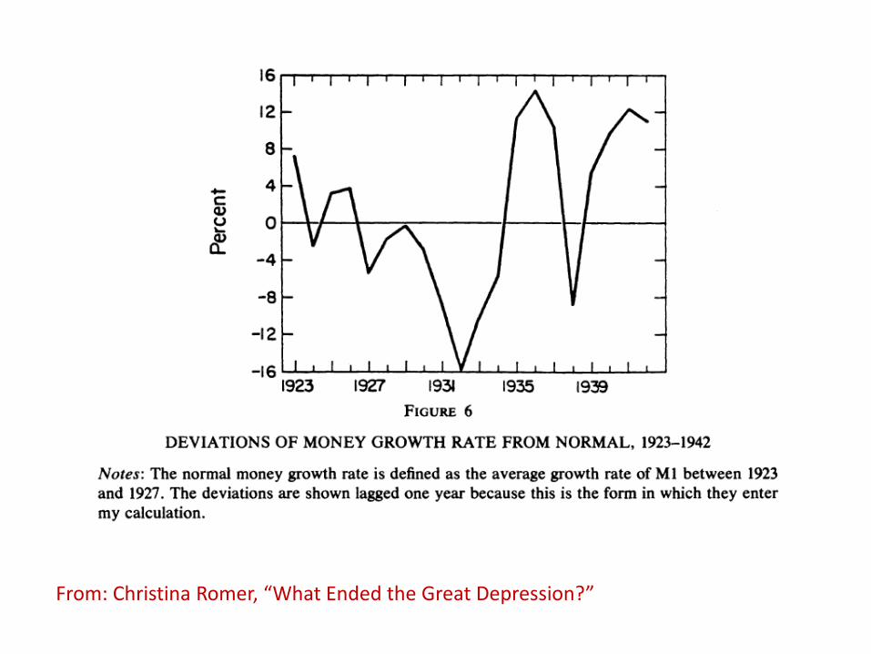
From: Christina Romer, “What Ended the Great Depression?”

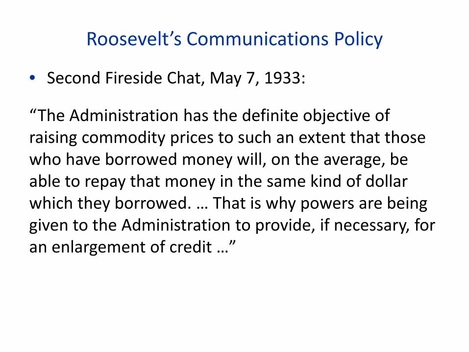
Roosevelt’s Communications Policy

• Second Fireside Chat, May 7, 1933:

“The Administration has the definite objective of raising commodity prices to such an extent that those who have borrowed money will, on the average, be able to repay that money in the same kind of dollar which they borrowed. … That is why powers are being given to the Administration to provide, if necessary, for an enlargement of credit …”

Stock Prices

1.5

6.5

11.5

16.5

21.5

26.5

31.5

36.5

Jan-

27

Aug-

27

Mar

-28

Oct

-28

May

-29

Dec-

29

Jul-3

0

Feb-

31

Sep-

31

Apr-

32

Nov

-32

Jun-

33

Jan-

34

Aug-

34

Mar

-35

Oct

-35

May

-36

Dec-

36

Mon

thly

S&

P St

ock

Pric

e In

dex

Producer Price Index, All Commodities

2.3

2.4

2.5

2.6

2.7

2.8

2.9

Jan-

29

Aug-

29

Mar

-30

Oct

-30

May

-31

Dec-

31

Jul-3

2

Feb-

33

Sep-

33

Apr-

34

Nov

-34

Jun-

35

Jan-

36

Aug-

36

Mar

-37

Oct

-37

Prod

ucer

Pric

e In

dex,

Log

arith

ms

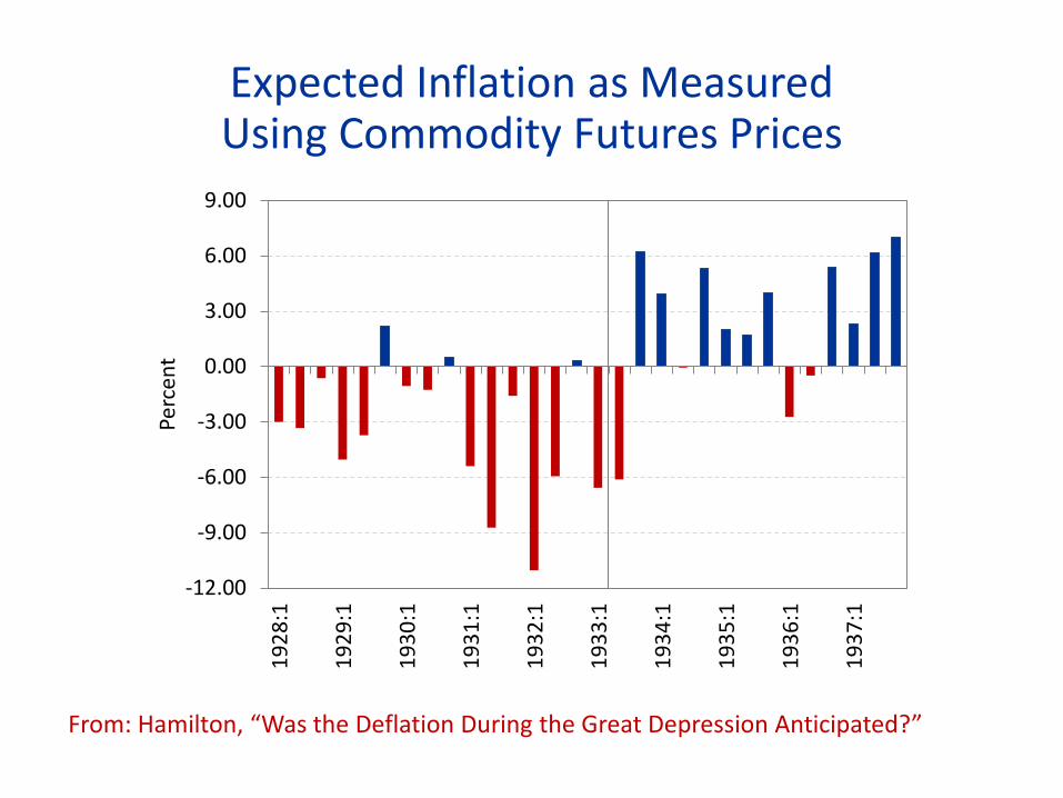
Expected Inflation as Measured Using Commodity Futures Prices

-12.00

-9.00

-6.00

-3.00

0.00

3.00

6.00

9.00

1928

:1

1929

:1

1930

:1

1931

:1

1932

:1

1933

:1

1934

:1

1935

:1

1936

:1

1937

:1

Perc

ent

From: Hamilton, “Was the Deflation During the Great Depression Anticipated?”

Devaluation in April 1933

Price of Cotton ($)

Exchange Rate ($ / ₤)

Pric

e of

Cot

ton,

in c

ents

Exch

ange

Rat

e

From: Temin and Wigmore, “The End of One Big Deflation”

From: Jalil and Rua, “Inflation Expectations and Recovery in Spring 1933”

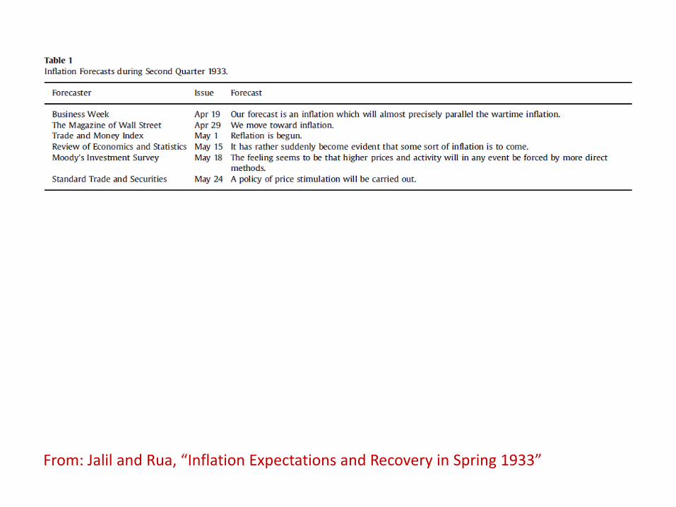
From: Jalil and Rua, “Inflation Expectations and Recovery in Spring 1933”

From: Jalil and Rua, “Inflation Expectations and Recovery in Spring 1933”

Truck Production, 1927-1936

0

10

20

30

40

50

60

70

80

90

100

Jan-

27Ju

l-27

Jan-

28Ju

l-28

Jan-

29Ju

l-29

Jan-

30Ju

l-30

Jan-

31Ju

l-31

Jan-

32Ju

l-32

Jan-

33Ju

l-33

Jan-

34Ju

l-34

Jan-

35Ju

l-35

Jan-

36Ju

l-36

Thou

sand

s of

Tru

cks

From: FRED, Federal Reserve Bank of St. Louis

Investment and Consumption Spending, 1932-33

Nondurables Consumption

Investment

From: Temin and Wigmore, “The End of One Big Deflation”

Evaluation

III. EGGERTSSON AND PUGSLEY, “THE MISTAKE OF 1937”

How Eggertsson and Pugsley Fit Into the Lecture

• Temin and Wigmore say a switch to an inflationary regime can be helpful at the ZLB

• Use April 1933 as an example.

• Eggertsson and Pugsley say a change in expectations of future policy away from reflation and expansion can be very damaging at the ZLB.

• Use 1937–38 recession as an example.

Industrial Production, 1926–1941

Alternative Explanations for the 1937–38 Recession

• Increase in reserve requirements (Friedman and Schwartz, Calomiris, Mason, and Wheelock)

• Sterilization of gold inflows (Irwin)

• Fiscal contraction

• Supply shocks (Hausman)

Eggertsson and Pugsley’s Explanation

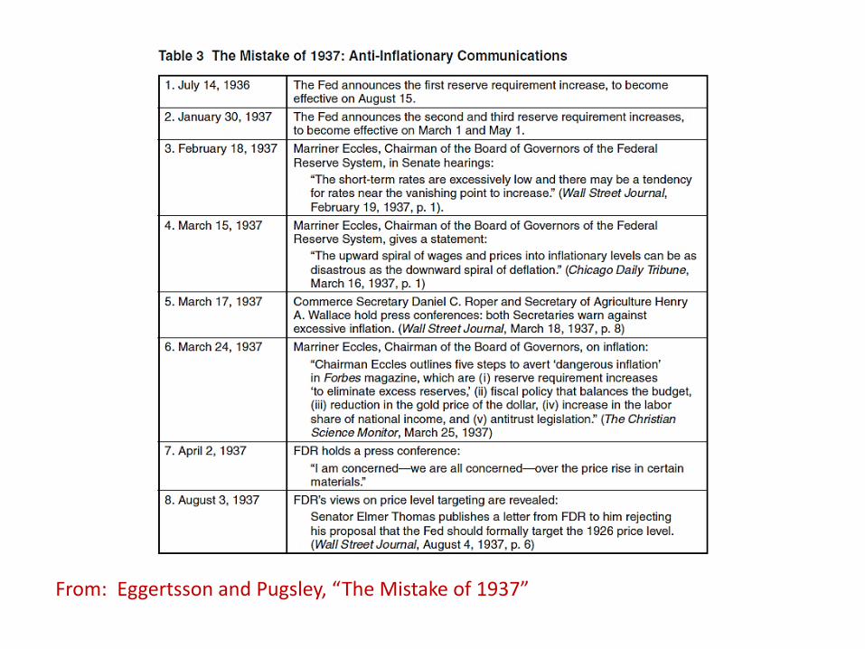
• Policymakers started expressing concern about inflation and deficits.

• Caused a negative change in expectations of future policy.

• This had contractionary effects on real activity.

Eggertsson and Pugsley’s Model

• DSGE model with binding zero lower bound due to real shocks.

• Calibrate model and find that inflation and output are extremely sensitive to changes in beliefs about future policy at ZLB. (Sensitivity is asymmetric.)

• Source of sensitivity is “contractionary spiral”—change in expectations in one instance affects expectations in other situations, and those expectations feed on each other (vicious feedback loop).

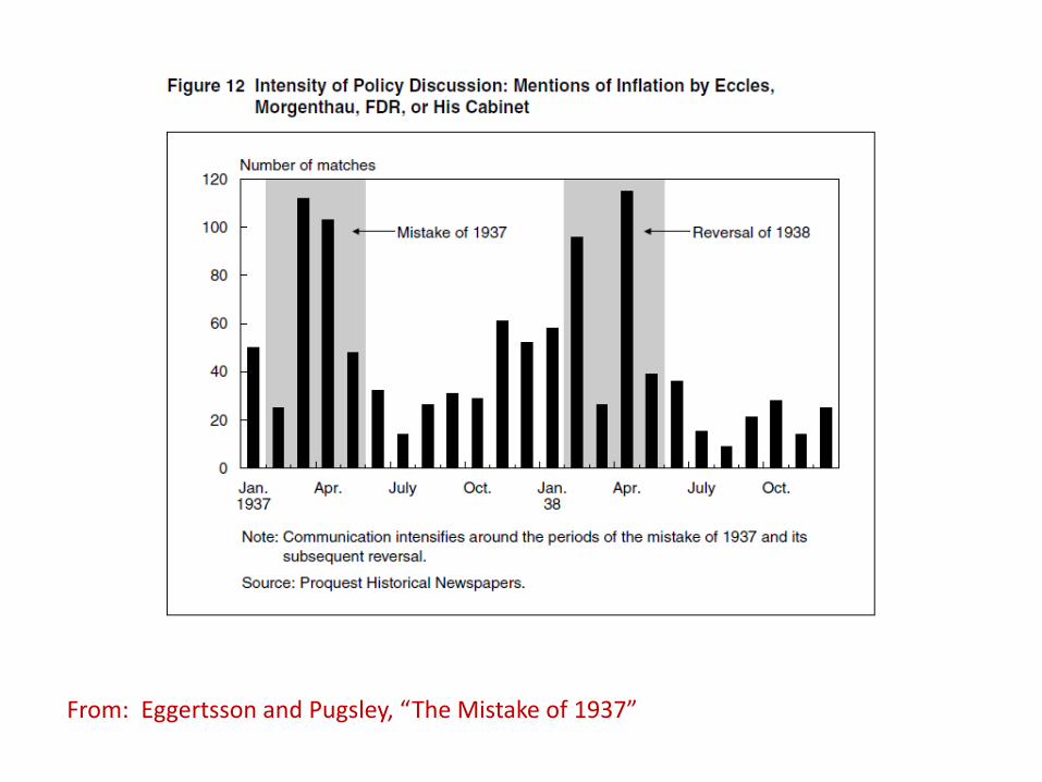
Eggertsson and Pugsley’s Evidence

• Narrative evidence from statements and actions.

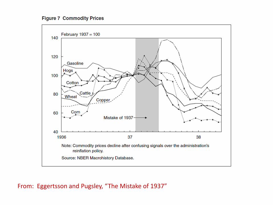
• Behavior of commodity prices.

• Behavior of long-rates relative to short rates.

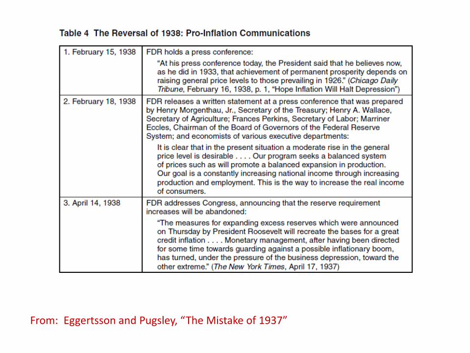
• The behavior of the economy when statements and actions changed back.

From: Eggertsson and Pugsley, “The Mistake of 1937”

From: Eggertsson and Pugsley, “The Mistake of 1937”

From: Eggertsson and Pugsley, “The Mistake of 1937”

From: Eggertsson and Pugsley, “The Mistake of 1937”

From: Eggertsson and Pugsley, “The Mistake of 1937”

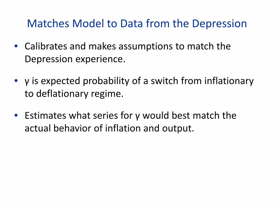
Matches Model to Data from the Depression

• Calibrates and makes assumptions to match the Depression experience.

• γ is expected probability of a switch from inflationary to deflationary regime.

• Estimates what series for γ would best match the actual behavior of inflation and output.

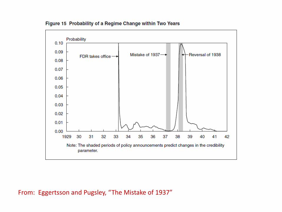
From: Eggertsson and Pugsley, “The Mistake of 1937”

Evaluation

IV. JOHANNES WIELAND, “ARE NEGATIVE SUPPLY

SHOCKS EXPANSIONARY AT THE ZERO LOWER BOUND?”

Motivation

• Standard models have counterintuitive implications at the zero lower bound (various “paradoxes”).

• A central implication of this type: An adverse supply shock, by raising expected inflation and so lowering the real interest rate, is expansionary at the zero lower bound.

• Wieland wants to test this prediction and investigate the implications of the results.

Key Questions

• Empirical: Are specific supply shocks (the Great Japan Earthquake, falls in oil supply) expansionary at the zero lower bound?

• Theoretical: If the answer is no, how broad are the implications? (For example, does it have implications for the fiscal multiplier at the zero lower bound? For measures to raise expected inflation through expectations of future monetary policy?)

Theory—Building Blocks

• New Keynesian IS curve:

�̇� 𝑡 = 𝑖 𝑡 − 𝜋 𝑡 − 𝜌.

• New Keynesian Phillips curve:

�̇� 𝑡 = 𝜌𝜋 𝑡 − κ∗[𝑦 𝑡 − 𝑦� 𝑡 ]

= 𝜌𝜋 𝑡 − κ∗ 𝑐 𝑡 − 𝑎 𝑡 ,

where a is productivity.

Theory—Implications for Levels

• Assume that in the long run, c = π = 0.

• New Keynesian IS curve:

𝑐(𝑡) = � 𝑖 𝑡 + 𝜏 − 𝜋 𝑡 + 𝜏 − 𝜌 𝑑𝜏∞

𝜏=0𝑡 .

• New Keynesian Phillips curve:

𝜋 𝑡 = κ∗ � 𝑒−𝜌𝜏[∞

𝜏=0𝑐 𝑡 + 𝜏 − 𝑎 𝑡 + 𝜏 ]𝑑𝜏.

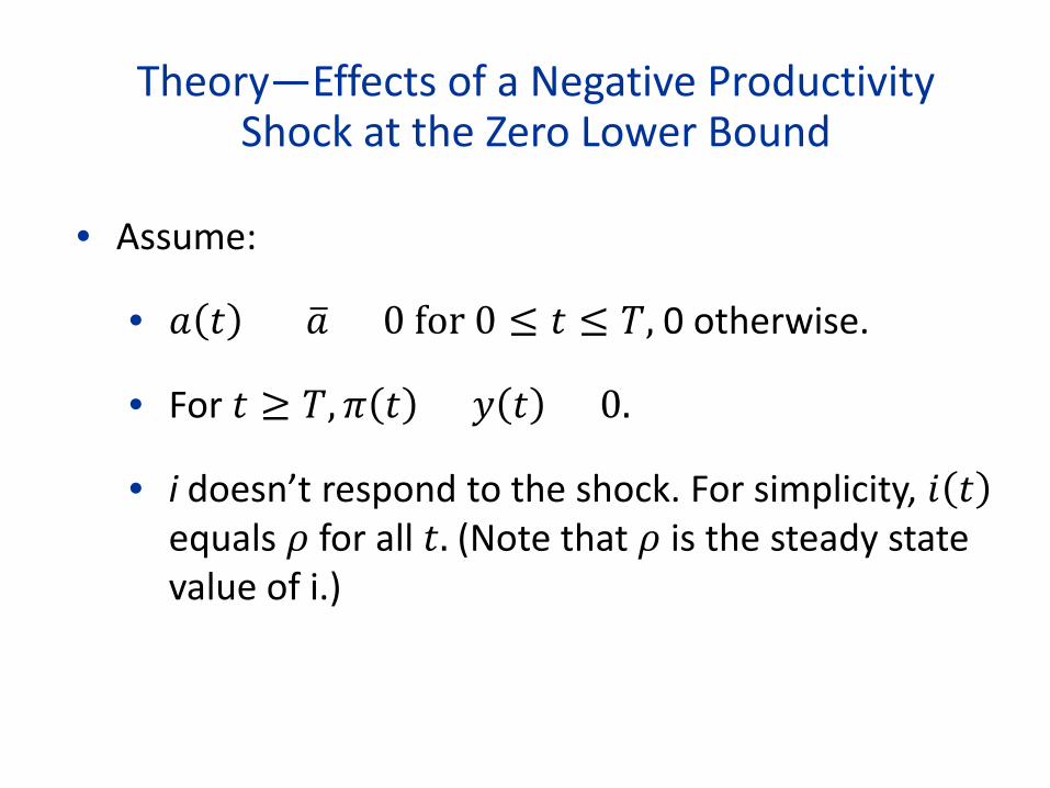
Theory—Effects of a Negative Productivity Shock at the Zero Lower Bound

• Assume:

• 𝑎 𝑡 = 𝑎� < 0 for 0 ≤ 𝑡 ≤ 𝑇, 0 otherwise.

• For 𝑡 ≥ 𝑇,𝜋 𝑡 = 𝑦 𝑡 = 0.

• i doesn’t respond to the shock. For simplicity, 𝑖 𝑡 equals 𝜌 for all 𝑡. (Note that 𝜌 is the steady state value of i.)

Effects of a Negative Productivity Shock at the ZLB

From: Wieland, “Are Negative Supply Shocks Expansionary at the Zero Lower Bound?”

Test 1: The Japanese Great Earthquake of March 2011

• Nominal interest rates fell slightly.

• Industrial production: Fell 15.8% from March to April (rose 1.9% from April to May).

• Real GDP: fell at a 5.9% annual rate in 2011Q1, and at a 2.1% annual rate in 2011Q2.

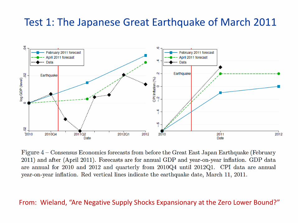
Test 1: The Japanese Great Earthquake of March 2011

From: Wieland, “Are Negative Supply Shocks Expansionary at the Zero Lower Bound?”

What Do We Learn from:

• The behavior of forecasts of inflation?

• The behavior of forecasts of real GDP?

• The actual behavior of output and inflation?

Test #2: Adverse Oil Supply Shocks

1. Adding oil price shocks to the baseline new Keynesian model.

2. Identifying oil supply shocks.

3. How oil prices and expected inflation behave following a shock.

4. Results.

Step 2: Identifying Oil Supply Shocks

• A VAR with a timing assumption: “I assume that oil production responds to other structural shocks (e.g., demand shocks) with at least a one-month delay.”

Step 3: How Oil Prices Behave Following a Shock

From: Wieland, “Are Negative Supply Shocks Expansionary at the Zero Lower Bound?”

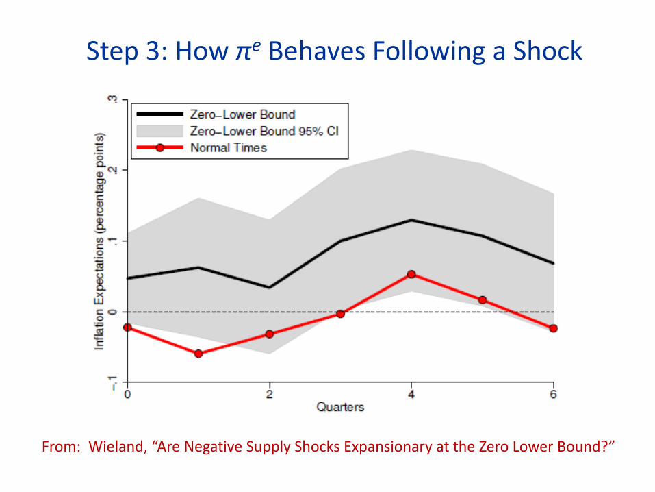
Step 3: How πe Behaves Following a Shock

From: Wieland, “Are Negative Supply Shocks Expansionary at the Zero Lower Bound?”

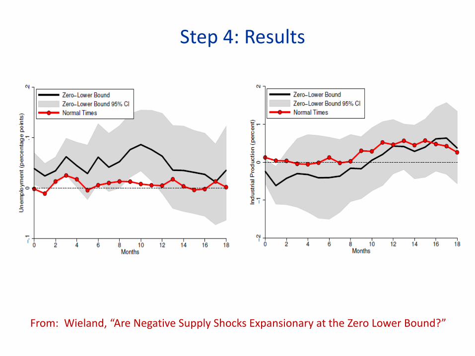
Step 4: Results

From: Wieland, “Are Negative Supply Shocks Expansionary at the Zero Lower Bound?”

Step 4: Results

From: Wieland, “Are Negative Supply Shocks Expansionary at the Zero Lower Bound?”

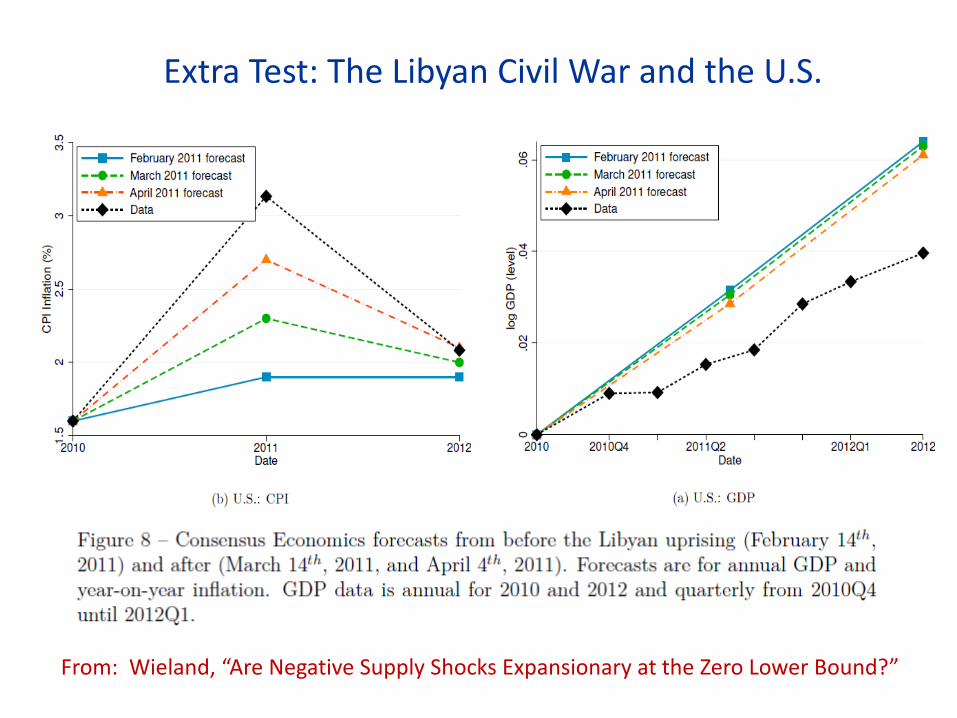
Extra Test: The Libyan Civil War and the U.S.

From: Wieland, “Are Negative Supply Shocks Expansionary at the Zero Lower Bound?”

Discussion

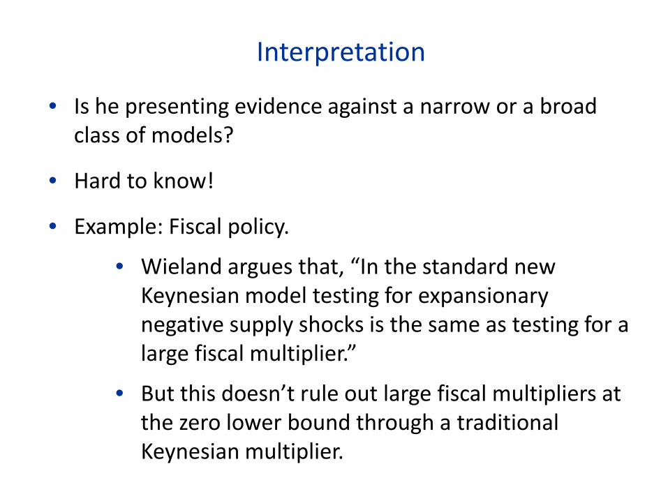
Interpretation

• Is he presenting evidence against a narrow or a broad class of models?

• Hard to know!

• Example: Fiscal policy.

• Wieland argues that, “In the standard new Keynesian model testing for expansionary negative supply shocks is the same as testing for a large fiscal multiplier.”

• But this doesn’t rule out large fiscal multipliers at the zero lower bound through a traditional Keynesian multiplier.

Other Possible Models

• Old Keynesian models?

• Models with credit constraints.

• Replacing the new Keynesian Philips curve with a sticky information Phillips curve.

• Other paths in the standard new Keynesian model.

• …?

V. A LITTLE ON ABENOMICS

Overview

• Shinzō Abe became Prime Minister in December 2012.

• Initial measures: • Change in leadership at Bank of Japan. • Change in inflation target (from 1% to 2%). • Doubling of monetary base, massive QE. • Deliberate depreciation of the yen.

• Many subsequent measures.

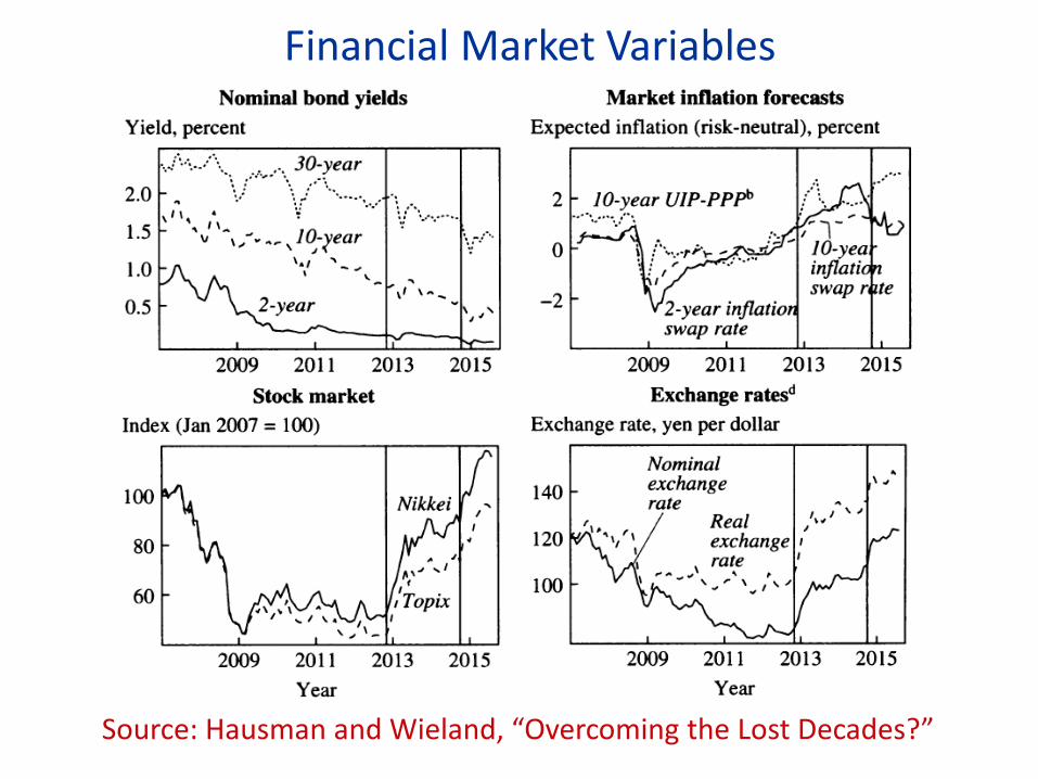
Financial Market Variables

Source: Hausman and Wieland, “Overcoming the Lost Decades?”

Source: Bank of Japan.

Inflation

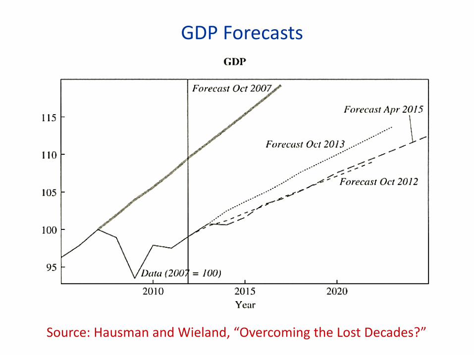
GDP Forecasts

Source: Hausman and Wieland, “Overcoming the Lost Decades?”

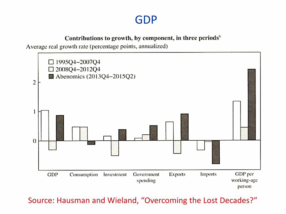
GDP

Source: Hausman and Wieland, “Overcoming the Lost Decades?”

Why Hasn’t Inflation Risen to 2%?

• Lack of credibility?

• A “timidity trap”? (Krugman)

• Other?