Lecture 7 Physical Processes for Diffuse Gas

1. Review & Preview2. Diffuse Gas Properties3. Cooling & Heating4. Ionization 5. Dielectric Recombination6. Charge Exchange7. Modeling & Examples

Partly covered by Dopita & Sutherland, Chs. 5-6

1. Review & PreviewCoverage so far (first 3 weeks):1. absorption lines, e.g. diffuse & translucent clouds2. emission lines, e.g., HII regions3. continuum emission, e.g., warm dustplus underlying radiative transfer & atomic processes

New material (next 3 weeks): general properties of galactic gas, which we already know is very diverse, i.e.,

nH ~ 10-3 – 106cm-3

T ~ 10 - 106 Kxe ~ 0 – 1

Initial focus: diffuse warmer gas (colder dense gas later).

2. Issue Raised By Diffuse GasGiven the wide range of physical properties, what simplifying concepts are applicable?

Long ago, Spitzer cited:1. Pressure Equilibrium

p = pth + pturb + pmag + pCRwith all terms roughly equal.

2. Phase Separation (by temperature and ionization fraction) as in the Field, Goldsmith, & Habing two-phase and the McKee & Ostriker three-phase models (inspired by Field’s 1965 work on thermal Instability of the interstellar gas).

The Phase AlphabetRecall the temperature-ionization classification form Lecture 1.We remember this by “multiplying” the T-letter by the xe-letter to get the phase name :

T xe Phase__________________________________H (>105 K) HI(M)

IWI(M)

W (102-104 K) X =WN(M)

NC (<102 K) CN(M)__________________________________

CI(M) & HN(M) are oxymorons

Key References for the Multiphase ISM

Field ApJ 142 531 1965Field, Goldsmith & Habing ApJ 155 L149 1969McKee & Ostriker ApJ 218 148 1977Wolfire et al. ApJ 587 278 2003

Heiles & Troland ApJ 586 1057 2003Heiles ASP 231, 294 2001

(also Heiles web site)

Dopita & Sutherland Ch. 14

3. Cooling & HeatingRecall from Lecture 4: To solve the heat equation for T, we need the heating & cooling functions Γ and Λ

Λ−Γ=dTdsTρ

A. Heating

Start by also recalling that the cooling function,

∑ ∑=−=Λul ul uluululululululc EnAEknknn β)(

simplifies in the low-density (sub-critical), optically-thin limit

Low Density Cooling function2

Hulul nλ=Λ

ulBulull

ucul TkTTTk

ggxx )/exp()()( −=λ

where x = abundance of the line coolantxc= abundance of collider

Tul = Eul / kB

The big unknown here is the collisional rate coefficients kul.

Famous cooling curve ofDalgarno & McCray, ARAA 10 375 1972

Fine-structure transitions

Forbidden lines

H lines

OVI etc. Fe ions

Bremsstrahlung

Λ / n2 plotted vs.T

Now unreliable; also inapplicable when lines are thermally excited or trapped, the likely situation at low T. Most useful for warm diffuse regions.

B. HeatingUnlike line cooling, which is reasonably well understood (despite our ignorance of many important collisional ratecoefficients), it is impossible to give a general treatment of heating. Recalling that heating (and cooling) refer to theenergy of the random or thermal motion of the gas, we can only list the general categories of heating:1. Radiative (UV & X-rays interactions with gas & dust)2. Cosmic rays3. Collisions with warmer dust4. Dissipation of mechanical energy (stellar winds & SNRs,

shocks, turbulence)5. Magnetic forces (ambipolar diffusion).

Each of these requires a detailed analysis of the energy source and the energy-dissipation process.

4. Ionization

There are three basic methods for ionizing the gas; 1. External ionizing radiation (UV & X-rays) 2. Cosmic rays3. Gas kinetic collisions

Cosmic rays are important only in cool & radiation-shielded regions (interstellar clouds), so for diffuse regions the competition is between radiative and collisional ionization.

The role of collisional ionization for ion X depends on the ratio of kBT to the ionization potential IP(X). Recall that

eVTTkB 605,11= )(397,12

λλAeVch

=

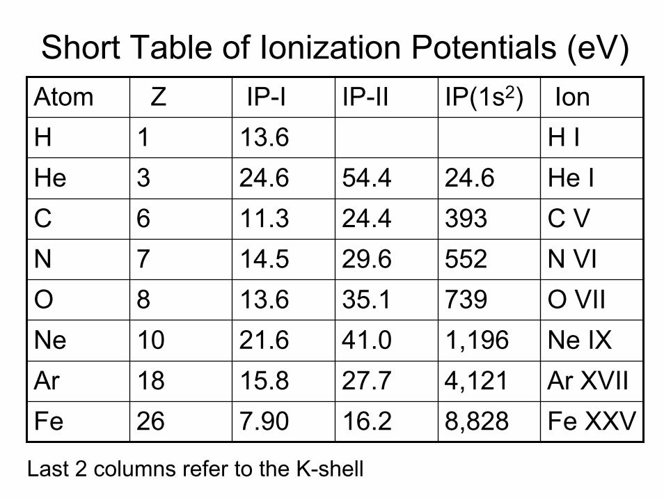
Short Table of Ionization Potentials (eV)Atom Z IP-I IP-II IP(1s2) IonH 1 13.6 H IHe 3 24.6 54.4 24.6 He IC 6 11.3 24.4 393 C VN 7 14.5 29.6 552 N VIO 8 13.6 35.1 739 O VIINe 10 21.6 41.0 1,196 Ne IXAr 18 15.8 27.7 4,121 Ar XVIIFe 26 7.90 16.2 8,828 Fe XXV

Last 2 columns refer to the K-shell

Collisional Ionization of Heavy IonsCross sections for electronic ionization are generally much larger than photoionization, but they are muchharder to calculate (even for H) and to measure for many energies of astrophysical interest.

σ

EIP

Useful reference for ionization cross sections: GS VoronovAtomic Data Nuclear Data TablesATNDT 65 1 1997

Would one expect the same shape at higherenergies or for target ions as neutral atoms?

Standard shape of an electronic ionizationor excitation cross section after Bethe.

Simplest Model of Collisional Ionization: H

Collisional ionization from ground state, rate coeff. k e + H → H+ + 2e

Radiative recombination, rate coeff. αe + H+→ H + hν

k = 4.76 X 10-11 cm3s-1 T1/2 exp(-157,891K / T) α2 = 2.47 X 10-13 cm3s-1 (T / 10,000 K)-0.8

Steady balance: α2 ne n(H+) = k ne n1 & n1 = nH – n(H+)with solution

αα/1

/)(k

kHxxe +== +

k/α = 0.062 at 8,000k/α = 4.28 at 10,000Valid near an HII region?

5. Dielectronic RecombinationRather than making a direct radiative transition on capture,

e + A+ → A* + hν,it may be more probable that a doubly-excited configuration A** is formed before radiating

e + A+ → A** → A* + hνa process known as dielectronic recombination. Above 10.000-20,000K, it is more important than the pure radiative recombination discussed so far. A** can also re-emit an electron (auto-ionization), but then this is not recombination.

References on recombination:Pequinot et al. A&A 251 680 1991Landini & Monsignori-Fossi A&AS 91 193 1991

Example of a reliable calculation of total recombinationcoefficients for Si+ and S++ (Nahar & Pradhan ApJ 447 966 1995). Older direct radiative coefficients are labeled “radiative”.

radiative radiative

6. Charge ExchangeElectronic recombination is a slow process, e.g., from Lecture 3

α2 (8000K,H) = 3 X 10-13 cm3 s-1.

Particle reactions are often many orders of magnitude larger, e.g., fast charge exchange of an ion and an abundant neutral is more important than recombination with electrons.

Perhaps the most important example for cool & warm regions isthe near-resonant (atypical) process

O+ + H →H+ + O H+ + O →O+ + H (exothermic) (endothermic)

But the IP difference between O and H, 0.020 eV, is ~ same as the fine-structure splitting of the O ground state:

Fine Structure Levels of OI

3P0 ____________ 326 K145.52µm

3P1 ____________ 228K 4S3/2 ___________227K

63.184µm

3P2 ____________ 0

O (+ H+) O+ (+ H)Σ g = 9 Σ g = 4 x 2 = 8

The O+/O RatioFor T >> 300K, the exponential in the Milne relation between the forward (exothermic) and backward (endothermic) reactions is ~ unity; only the statistical weights matter:

k(H+ + O) = (9/8) k(O+ + H) ( T >> 300K ).If O+ is only produced and destroyed by charge-exchange reactions, steady balance reads:

k(H+ + O) n(H+) n(O) = k(O+ + H) n(O+) n(H) .

Therefore the O/O+ ratio is the H+/H ratio multiplied by the ratio of rate coefficients:

)300()()(

89

)()(

)()(

)()( KT

OnHn

OnHn

HOkOHk

HnOn

>>→++

= +

+

+

+

+

+

+

+

Definitive Calculation of O+ + H Charge Exchange

Kingdon & Ferland (1996)

Field & Steigman (1971)

Note different scalesIn upper & lower panels

PC Stancil et al. A&AS 140 225 1999

There are large deviations from the 9/8 ratio below 300 K.

7. Applications - Collisional Ionization Models

Shapiro & Moore ApJ 207 460 1976Classic calculation of steady balance of collisional ionization and recombination for T > 104K. Line cooling calculated in the optically thin limit; no dust.

Fractional abundance of ionization stage vs. T.

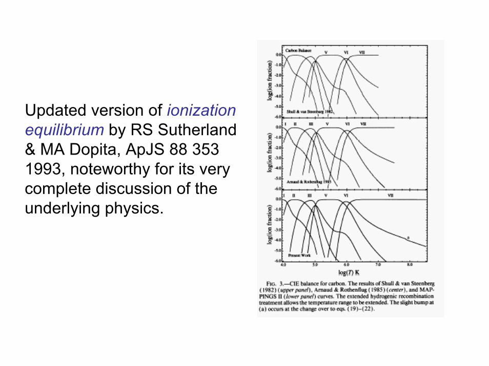
Updated version of ionization equilibrium by RS Sutherland& MA Dopita, ApJS 88 353 1993, noteworthy for its very complete discussion of the underlying physics.

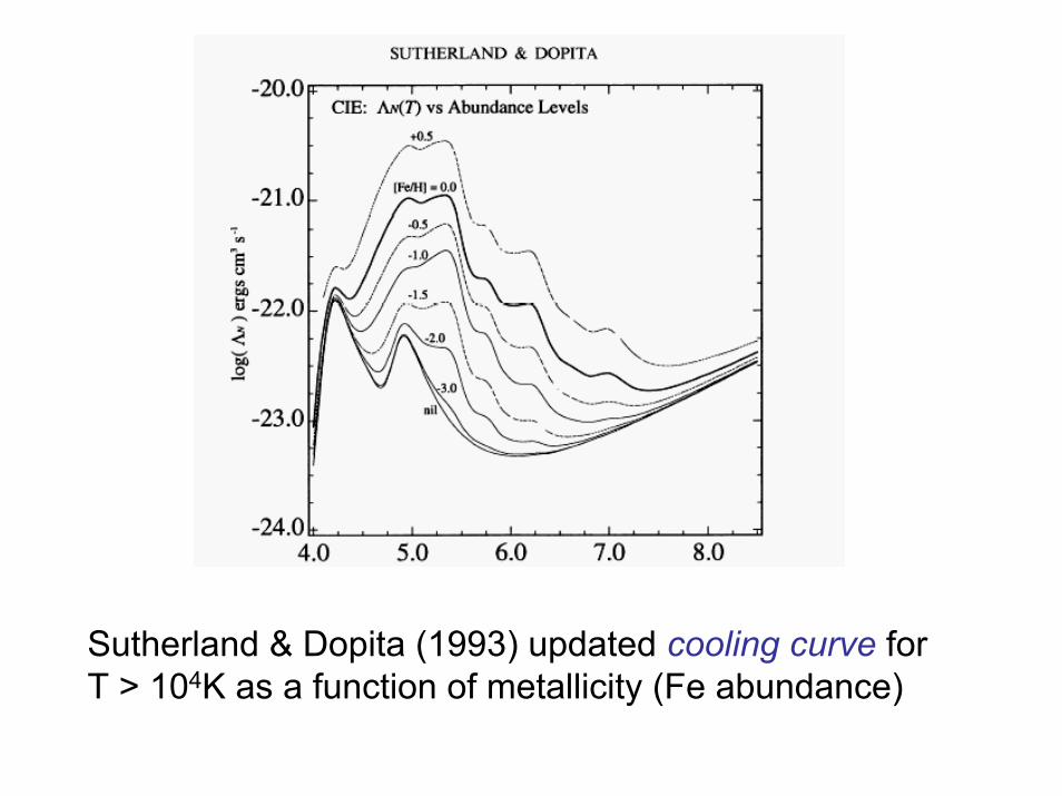
Sutherland & Dopita (1993) updated cooling curve for T > 104K as a function of metallicity (Fe abundance)

7B. Next Simplest Ionization ModelWe go beyond the model of Sec. 4 and include photo-ionization of H as well as collisional ionization and radiative recombination. The objective is to clarify the difference between photoionization and collisional models. The steady balance equations

α2 ne n(H+) = (k ne + G) n1n1 = nH – n(H+) & ne = n(H+)

lead to a quadratic equation:

(α2 + k)xe2 + (G/nH –k)ne – G/nH = 0

The photoionization rate G enters only via G/nH, the “ionization parameter”.

The solutions have the right limits: For small G/nH, we get the result of Sec. 4 (collisional ionization limit), and for large G/nH, e get xe = 1. We can estimate G/nH for a Stromgren model:

An O6 star outputs 2x1049 s-1 ionizing photons for a fluxF = 3 x 1011 cm-2s-1 at RS. Using the cross section at the Lyman limit, 6 x10-18 cm2, gives

G = 2 x 10-6 s-1 (RS/r)2

and G/n = 2 x 10-9 s-1 (RS/r)2 (1000 cm-3/nH).

In this density range, this ratio is larger than other relevant rate coefficients, confirming that this HIIregion is reasonably well described by a simple photoionization model.

What might be the next steps in making better models?

7C. Programs to Put It All Together For quantitative results of photoionization and collisional ionization models, and especially combined models withfull coverage of radiative and collisional processes, large computer programs are needed, e.g., one of the popular programs:

CLOUDY (Gary Ferland et al.) at www.nublado.org

XSTAR (Tim Kallmann) athttp://heasarcsfc.nasa.gov/docs/software/xstar.html

Warning: it’s important to understand the structural models in these programs and to be aware that the physics is not always up to date.