lecture 7 (linear motors ii) - overhead

8/10/2019 Lecture 7 (Linear Motors II) - Overhead

http://slidepdf.com/reader/full/lecture-7-linear-motors-ii-overhead 1/8

University of British Columbia Elec Machines & Electronics

EECE 365 – Winter 2013 Lecture 7: Linear Machines II

Nathan Ozog © 2013 of 8

Linear Machines

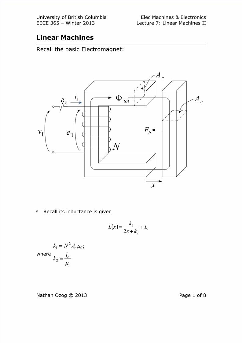
Recall the basic Electromagnet:

Recall its inductance is given

( ) l Lk x

k x L +

+=

2

1

2

where

r

c

c

l k

A N k

µ

µ

=

=

2

02

1 ;

1i

1e

N

g R

x

c A

b F

tot Φ

1v

c A






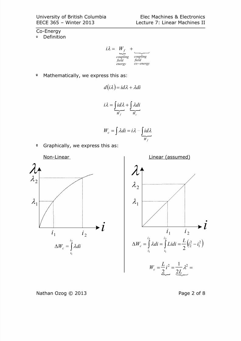
Co-Energy

Definition

{ 321

energyco field

coupling

energy field

coupling

f W i

−

+=λ

Mathematically, we express this as:

( )

{ {

{

f

c f

W

c

W W

id idiW

diid i

diid id

∫∫

∫∫

−==

+=

+=

λ λ λ

λ λ λ

λ λ λ

Graphically, we express this as:

Non-Linear Linear (assumed)

λ

i

2λ

1λ

1i

2i

∫=∆2

1

i

i

c diW λ ( )2

1

2

22

2

1

2

1

ii L

LididiW i

i

i

i

c −===∆ ∫∫λ

{

===321

22

2

1

2λ L

i L

W c

λ

i

2λ

1λ

1i 2i






For a linear system, energy and co-energy will be equal

They are often both simply referred to as “energy”

Recalling our system, we note that the relationship between current andflux in the magnet changes with the position

i.e. ( ) xih ,=λ

The co-energy in the magnet is also “ ”It does not depend on the of flux or current, only on their

present state and relationship

the equation for change in co-energy in the magnet is:

( )( )

( )( )

−=∆ ∫∫ab xi

a

xi

bc di xidi xiW 00

,, λ λ

- -

( )a xih ,

( )b xih ,






This time, we consider the force on the bar when current is held constant

i.e. aii =

f

t

t

x

x

W iedt fdxb

a

b

a

∆−= ∫∫

dt

d e

λ = , because flux will change

so, there is addition of electrical energy as the bar moves

f

t

t

x

x

W iedt fdxb

a

b

a

∆−= ∫∫

Consider the change in electrical energy graphically

Position a Position b






The total change is:

Mathematically, we have

( )=−====∆ ∫∫∫ ab

t

t

t

t

e id idt dt

d iiedt W

b

a

b

a

b

a

λ λ λ λ

λ

λ

A subtle note:Current and flux are not functions of each-other in this equation






Next consider the energy in the coupling field

We again have

( ) ( )

−=∆ ∫∫

ab xi xi

f id id W

,

0

,

0

λ λ

λ λ

Graphically:

Position a Position b

( ) ( )

=

−=∆ ∫∫ab xi xi

f id id W

,

0

,

0

λ λ

λ λ






( ) ( )

c

x

x

AD

xi

BC

xi

ABCD

t

t

x

x

f em

W fdx

id id iedt fdx

W W W

b

a

abb

a

b

a

∆=

−−=

∆−∆=∆

∫

∫∫∫∫321321321

0

,

0

0

,

0

λ λ

λ λ

Remember that ∫= diW c λ

So

( ) ( )

( ) ( )[ ]∫

∫∫

−=

−=∆

a

aa

i

ab

i

a

i

bc

di xi L xi Li

dii xdii xW

0

00

,,

,, λ λ






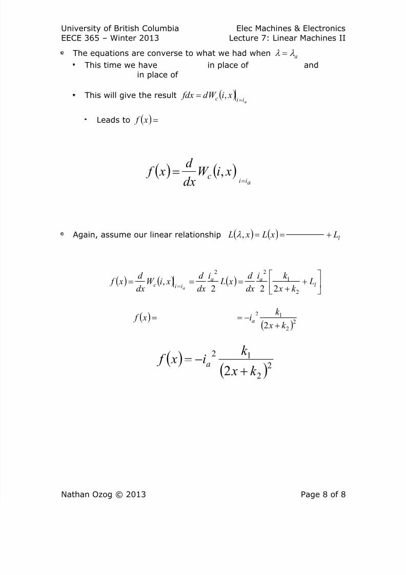
The equations are converse to what we had when aλ λ =

This time we have in place of and

in place of

This will give the result ( )aiic

xiW d fdx=

= ,

Leads to ( )= x f

Again, assume our linear relationship ( ) ( ) l L x L x L +==,λ

( ) ( ) ( )

+

+===

= l aa

iic Lk x

k i

dx

d x L

i

dx

d xiW

dx

d x f

a2

1

22

222,

( )( )22

12

2 k x

k i x f a

+−==

( )( )22

12

2 k x

k i x f a

+−=

( ) ( )aii

xiW dx

d x f c

== ,

lecture 7 (linear motors ii) - overhead

Documents