lecture 6- cpu scheduling continued - profiles @ iiit...

Lecture 6- CPU Scheduling Continued

Instructor : Bibhas Ghoshal ([email protected])

Autumn Semester, 2015

Bibhas Ghoshal IOSY 332C & IOPS 332C: OS Autumn Semester, 2015 1 / 24

Shortest Remaining Job First (SRJF)

Preemptive version of SJFWhile a job A is running, if a new job B comes whose length isshorter than the remaining time of job A, then B preempts A and Bis started to run.


SRJF-Example

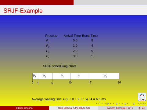
Process Arrival Time Burst Time

P1 0.0 8

P2 1.0 4

P3 2.0 9

P4 3.0 5

SRJF scheduling chart

Average waiting time = (9 + 0 + 2 + 15) / 4 = 6.5 ms

P2P1

1 170 5

P1

26

P4

10

P3


Numerical Example

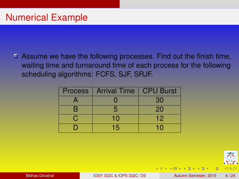
Assume we have the following processes. Find out the finish time,waiting time and turnaround time of each process for the followingscheduling algorithms: FCFS, SJF, SRJF.

Process Arrival Time CPU BurstA 0 30B 5 20C 10 12D 15 10


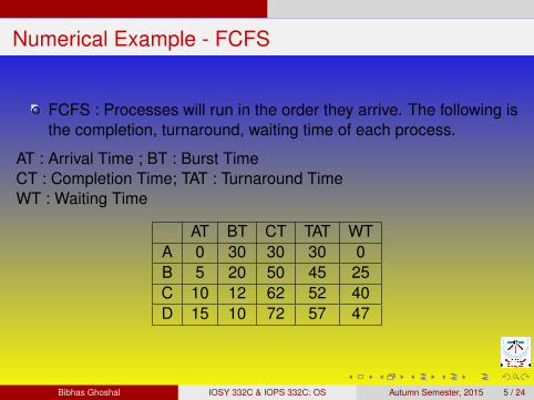
Numerical Example - FCFS

FCFS : Processes will run in the order they arrive. The following isthe completion, turnaround, waiting time of each process.

AT : Arrival Time ; BT : Burst TimeCT : Completion Time; TAT : Turnaround TimeWT : Waiting Time

AT BT CT TAT WTA 0 30 30 30 0B 5 20 50 45 25C 10 12 62 52 40D 15 10 72 57 47


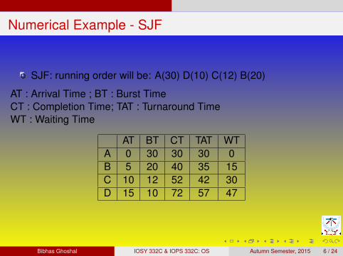
Numerical Example - SJF

SJF: running order will be: A(30) D(10) C(12) B(20)




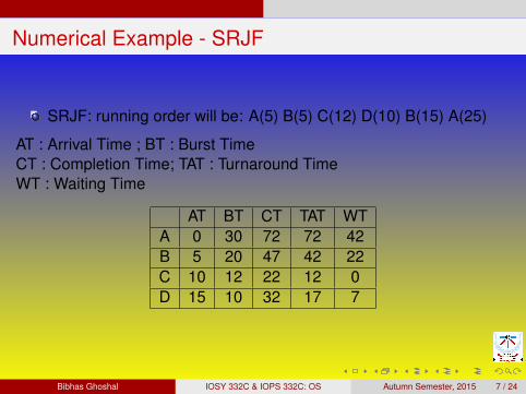
Numerical Example - SRJF

SRJF: running order will be: A(5) B(5) C(12) D(10) B(15) A(25)




Priority Scheduling

A priority number (integer) is associated with each processThe CPU is allocated to the process with the highest priority(smallest integer is equivalent to highest priority)

Preemptive - higher priority process preempts the running onenonpreemptive

SJF is a priority scheduling where priority is the predicted nextCPU burst timeProblem : Starvation – low priority processes may never executeSolution : Aging – as time progresses increase the priority of theprocess


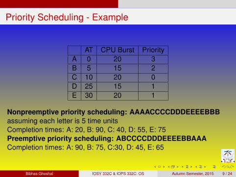
Priority Scheduling - Example

AT CPU Burst PriorityA 0 20 3B 5 15 2C 10 20 0D 25 15 1E 30 20 1

Nonpreemptive priority scheduling: AAAACCCCDDDEEEEBBBassuming each letter is 5 time unitsCompletion times: A: 20, B: 90, C: 40, D: 55, E: 75Preemptive priority scheduling: ABCCCCDDDEEEEBBAAACompletion times: A: 90, B: 75, C:30, D: 45, E: 65


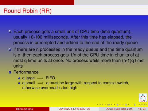
Round Robin (RR)

Each process gets a small unit of CPU time (time quantum),usually 10-100 milliseconds. After this time has elapsed, theprocess is preempted and added to the end of the ready queueIf there are n processes in the ready queue and the time quantumis q, then each process gets 1/n of the CPU time in chunks of atmost q time units at once. No process waits more than (n-1)q timeunitsPerformance

q large =⇒ FIFOq small =⇒ q must be large with respect to context switch,otherwise overhead is too high


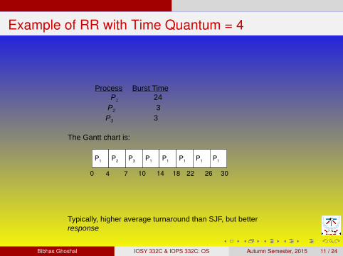
Example of RR with Time Quantum = 4

Process Burst TimeP1 24

P2 3 P3 3

The Gantt chart is:

Typically, higher average turnaround than SJF, but better response

P1 P2 P3 P1 P1 P1 P1 P1

0 4 7 10 14 18 22 26 30


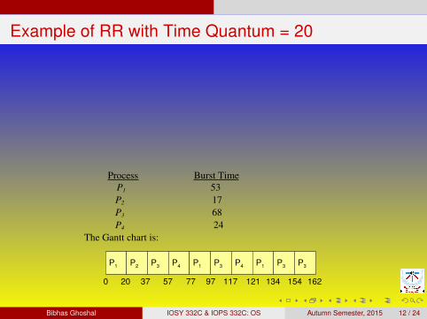
Example of RR with Time Quantum = 20

Process Burst Time P1 53

P2 17 P3 68 P4 24

The Gantt chart is:

Typically, higher average turnaround than SJF, but better response

P1 P2 P3 P4 P1 P3 P4 P1 P3 P3

0 20 37 57 77 97 117 121 134 154 162


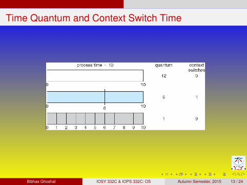
Time Quantum and Context Switch Time


Turnaround Time Varies With The Time Quantum


Multilevel Queue

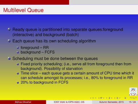
Ready queue is partitioned into separate queues:foreground(interactive) and background (batch)Each queue has its own scheduling algorithm

foreground – RRbackground – FCFS

Scheduling must be done between the queuesFixed priority scheduling; (i.e., serve all from foreground then frombackground). Possibility of starvationTime slice – each queue gets a certain amount of CPU time which itcan schedule amongst its processes; i.e., 80% to foreground in RR20% to background in FCFS


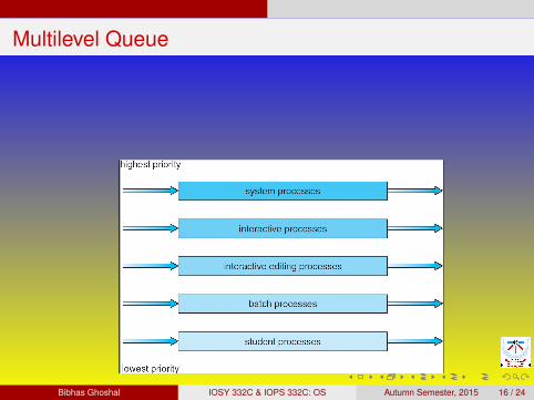
Multilevel Queue


Multilevel Feedback Queue

A process can move between the various queues; aging can beimplemented this wayMultilevel-feedback-queue scheduler defined by the followingparameters:

number of queuesscheduling algorithms for each queuemethod used to determine when to upgrade a processmethod used to determine when to demote a processmethod used to determine which queue a process will enter whenthat process needs service


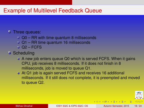
Example of Multilevel Feedback Queue

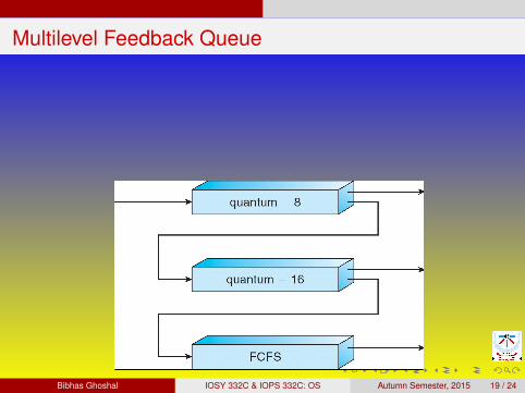
Three queues:Q0 – RR with time quantum 8 millisecondsQ1 – RR time quantum 16 millisecondsQ2 – FCFS

SchedulingA new job enters queue Q0 which is served FCFS. When it gainsCPU, job receives 8 milliseconds. If it does not finish in 8milliseconds, job is moved to queue Q1.At Q1 job is again served FCFS and receives 16 additionalmilliseconds. If it still does not complete, it is preempted and movedto queue Q2.


Multilevel Feedback Queue


Multiple-Processor Scheduling

CPU scheduling more complex when multiple CPUs are availableHomogeneous processors within a multiprocessorLoad sharing : Preserve locality of data and stateAsymmetric multiprocessing – only one processor accesses theoperating system data structures, alleviating the need for kerneldata sharing among processorsSome cooperative processes like to run with n processors or noneat all : Gang scheduling to assign group of processors


Real Time Scheduling

Hard real-time systems – required to complete a critical taskwithin a guaranteed amount of timeSoft real-time computing – requires that critical processes receivepriority over less fortunate onesIn both cases, RT behaviour is achieved by dividing the programinto number of process, each of whose behaviour is predictable.When an external event is detected, it is the job of the scheduler toschedule the processes in such a way that all deadlines are met.The events a RT system has to handle are periodic(occuring atregular intervals) or aperiodic(occuring unpredictably)If there are m periodic events and event i occurs with period Piand requires Ci seconds of CPU to handle each event, then theload can be handled if

∑mi=1

CiPi≤ 1 - schedulable RT system


Thread Scheduling

Local Scheduling – How the threads library decides which threadto put onto an available light weight process (LWP) (kernel thread)Global Scheduling – How the kernel decides which kernel threadto run next


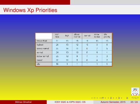
Windows Xp Priorities


Linux Scheduling

Two algorithms: time-sharing and real-timeTime-sharing

Prioritized credit-based – process with most credits is schedulednextCredit subtracted when timer interrupt occursWhen credit = 0, another process chosenWhen all processes have credit = 0, recrediting occurs

Real TimeSofty real timePosix.1b compliant – two classes

FCFS and RRHighest Priority Process always run first


lecture 6- cpu scheduling continued - profiles @ iiit...

Documents