lecture 5 economic growth: optimal growth model … is missing? topics in modern growth...
TRANSCRIPT

What is missing? Topics in modern growth theory Optimal growth model Endogenous growth
Lecture 5Economic Growth: Optimal growth model and
endogenous growth
Leopold von ThaddenUniversity of Mainz and ECB (on leave)
Macroeconomics II, Summer Term 2013
1 / 54

What is missing? Topics in modern growth theory Optimal growth model Endogenous growth
I What is missing? Topics in modern growth theory
Goal:
This lecture gives an introduction to various questions addressed inmodern growth theory
As shown in the previous lecture from a number of perspectives, theability of the Solow-model, when narrowly specified, to accountquantitatively for empirical growth patterns both within and betweencountries is not fully satisfactory
Consequently, new lines of research have emerged which:
→ 1) modify the role of capital in the original Solow model
→ 2) focus on different and endogenously derived sources of growth
→ 3) allow for a more nuanced discussion of convergence
2 / 54
What is missing? Topics in modern growth theory Optimal growth model Endogenous growth
I What is missing? Topics in modern growth theory
1) Modifying the role of capital:
Starting point: Quantitative implications of Solow-model are not satisfactoryif one assumes that the contribution of capital to output is fully captured bythe private return earned by physical capital
(Main) Extensions:(i) Accumulation of physical capital subject to externalities such that theeconomy-wide (or social) return to capital exceeds the private return(ii) Parallel focus on human and physical capital allows for a moreencompassing role of capital
→ Such extensions do a much better job to account for cross-countryvariations in per capita incomes
3 / 54

What is missing? Topics in modern growth theory Optimal growth model Endogenous growth
I What is missing? Topics in modern growth theory
2) Focus on different and endogenously derived sources of growth
Starting point:→ Solow-model treats the ’effectiveness of labour’(ie At ) as a black box: thecore variable which explains long-run per capita growth is exogenously given→ This approach is not satisfactory: growth should not occur by assumption,but it should rather be endogenously explained within the model - in particular,in view of lasting growth differentials between countries which seek explanation
Model extensions allow for various interpretations of At relating, among otherthings, to the diffusion of knowledge, the role of education and skills, the roleof property rights, the quality of infrastructure etc.
→ In line with such interpretations, endogenous growth theory establishesmechanisms which replace the exogeneity of At against alternative engines oflong-run growth, linked to country-specific fundamentals and variables that canbe affected by policy decisions
4 / 54
What is missing? Topics in modern growth theory Optimal growth model Endogenous growth
I What is missing? Topics in modern growth theory
2) Focus on different and endogenously derived sources of growth
Comment:
As recognized by the first generation of endogenous growth models,extensions of type 1) and 2) can well be combined, ie the accumulation ofcapital, when suffi ciently broadly modelled, can maintain long-run percapita growth in the absence of growth through At
Key requirement: the broad measure of capital must not be subject todiminishing (social) returns, but rather to constant returns to scale(see: Jones and Manuelli, 1990; Lucas, 1988; Rebelo, 1991; Romer, 1986)
5 / 54

What is missing? Topics in modern growth theory Optimal growth model Endogenous growth
I What is missing? Topics in modern growth theory
3) More nuanced discussion of convergence
Starting point: The absence of absolute convergence of per capita incomes isconsistent with two alternative views:
View I): Absence of any convergence or, alternatively,View II): Existence of conditional convergence
View I): Absence of any convergence:→ Countries can grow permanently at different per capita growth rates
6 / 54
What is missing? Topics in modern growth theory Optimal growth model Endogenous growth
I What is missing? Topics in modern growth theory
3) More nuanced discussion of convergence
View II) : Existence of conditional convergence→ Countries are characterized by country-specific fundamentals (like savingsrates and income shares) and, hence, by country-specific balanced growth paths→ Convergence takes place conditional on these country-specific fundamentals
Example 1: Consider 2 ‘poor countries’with identical starting positions interms of capital endowments per worker (ie K/N), but different savings rates.→ The countries will have different growth rates during the catching-up phase→ Conditional on the different values of s (which imply different steady-statevalues k#So (si ), i = 1, 2), the statement that ‘poor countries should grow fasterthan rich countries’remains correct
7 / 54

What is missing? Topics in modern growth theory Optimal growth model Endogenous growth
I What is missing? Topics in modern growth theory
3) More nuanced discussion of convergence
View II) : Existence of conditional convergence
Example 2: The hypothesis of absolute convergence has some support for asmall number of OECD-countries for the post WW-II catching-up phase (butnot for larger samples of countries)→ Since these countries are fundamentally very similar, this observation isconsistent with conditional convergence
Implication of view II: in the long run, countries display identical per capitagrowth rates, but different levels of per capita incomes
8 / 54
What is missing? Topics in modern growth theory Optimal growth model Endogenous growth
I What is missing? Topics in modern growth theory
3) More nuanced discussion of convergence
View I vs. View II:To distinguish between these 2 views empirically is challenging sincefundamentals themselves may change over time
‘Controversy’:→ In those poor countries which fail to catch-up fundamentals may haveworsened, while they may have further improved in a number of countrieswhich are already richnotice: this interpretation (which emphasizes the role of transitional dynamics)is in the spirit of the Solow-model→ At the same time: rich countries may benefit from permanently higher percapita growth ratesnotice: this interpretation is in the spirit of endogenous growth theories
9 / 54

What is missing? Topics in modern growth theory Optimal growth model Endogenous growth
I What is missing? Topics in modern growth theory
Comment:
→ we will return to the concept of endogenous growth at the end of this lecture
→ but we will analyze first the ‘standard’model of optimal growth withlabour-augmenting technological progress and compare it with the Solow-model
→ this is advisable, since most models of endogenous growth are variations ofthe ‘standard’optimal growth model
10 / 54
What is missing? Topics in modern growth theory Optimal growth model Endogenous growth
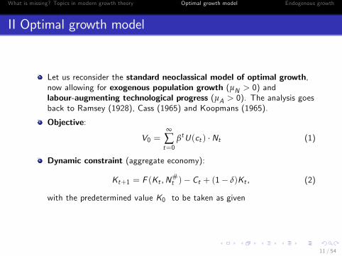
II Optimal growth model
Let us reconsider the standard neoclassical model of optimal growth,now allowing for exogenous population growth (µN > 0) andlabour-augmenting technological progress (µA > 0). The analysis goesback to Ramsey (1928), Cass (1965) and Koopmans (1965).
Objective:
V0 =∞
∑t=0
βtU(ct ) ·Nt (1)
Dynamic constraint (aggregate economy):
Kt+1 = F (Kt ,N#t )− Ct + (1− δ)Kt , (2)
with the predetermined value K0 to be taken as given
11 / 54
What is missing? Topics in modern growth theory Optimal growth model Endogenous growth
II Optimal growth model
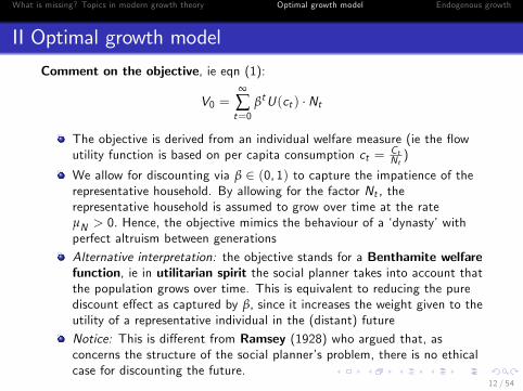
Comment on the objective, ie eqn (1):
V0 =∞
∑t=0
βtU(ct ) ·Nt
The objective is derived from an individual welfare measure (ie the flowutility function is based on per capita consumption ct =
CtNt)
We allow for discounting via β ∈ (0, 1) to capture the impatience of therepresentative household. By allowing for the factor Nt , therepresentative household is assumed to grow over time at the rateµN > 0. Hence, the objective mimics the behaviour of a ‘dynasty’withperfect altruism between generations
Alternative interpretation: the objective stands for a Benthamite welfarefunction, ie in utilitarian spirit the social planner takes into account thatthe population grows over time. This is equivalent to reducing the purediscount effect as captured by β, since it increases the weight given to theutility of a representative individual in the (distant) future
Notice: This is different from Ramsey (1928) who argued that, asconcerns the structure of the social planner’s problem, there is no ethicalcase for discounting the future.
12 / 54
What is missing? Topics in modern growth theory Optimal growth model Endogenous growth
II Optimal growth model
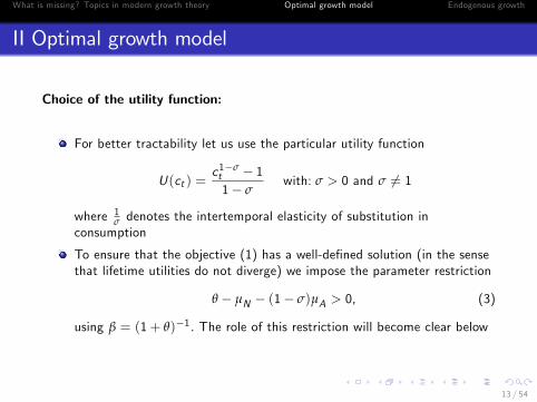
Choice of the utility function:
For better tractability let us use the particular utility function
U(ct ) =c1−σt − 11− σ
with: σ > 0 and σ 6= 1
where 1σ denotes the intertemporal elasticity of substitution in
consumption
To ensure that the objective (1) has a well-defined solution (in the sensethat lifetime utilities do not diverge) we impose the parameter restriction
θ − µN − (1− σ)µA > 0, (3)
using β = (1+ θ)−1. The role of this restriction will become clear below
13 / 54

What is missing? Topics in modern growth theory Optimal growth model Endogenous growth
II Optimal growth model
Transformation of c into units of effective labour:
From the analysis of the Solow-model we anticipate that the steady-statesolution will involve variables expressed in terms of units of effectivelabour
Hence, we usect = At · c#t = (1+ µA)
t · A0 · c#t
14 / 54

What is missing? Topics in modern growth theory Optimal growth model Endogenous growth
II Optimal growth model
Incorporating these features, the objective (1) can be rewritten as
∞
∑t=0
βt · (ct )1−σ − 11− σ
·Nt
=∞
∑t=0
βt · ((1+ µA)t · A0 · c#t )1−σ − 11− σ
·Nt
=∞
∑t=0[β · (1+ µN )]
t · ((1+ µA)t · A0 · c#t )1−σ − 11− σ
·N0, (4)
where the last step uses
Nt = (1+ µN )t ·N0
Consistent with eqn (5) of the previous Lecture, the dynamic constraint(2) can be expressed in units of effective labour:
k#t+1 · (1+ µN# ) = f (k#t )− c
#t + (1− δ)k#t (5)
15 / 54
What is missing? Topics in modern growth theory Optimal growth model Endogenous growth
II Optimal growth model
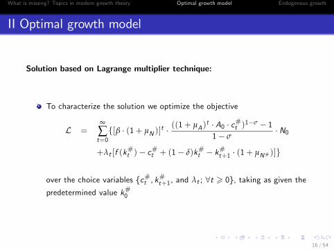
Solution based on Lagrange multiplier technique:
To characterize the solution we optimize the objective
L =∞
∑t=0{[β · (1+ µN )]
t · ((1+ µA)t · A0 · c#t )1−σ − 11− σ
·N0
+λt [f (k#t )− c
#t + (1− δ)k#t − k
#t+1 · (1+ µN# )]}
over the choice variables {c#t , k#t+1, and λt ; ∀t > 0}, taking as given the
predetermined value k#0
16 / 54
What is missing? Topics in modern growth theory Optimal growth model Endogenous growth
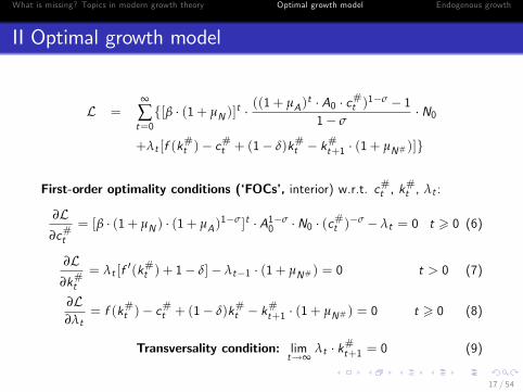
II Optimal growth model
L =∞
∑t=0{[β · (1+ µN )]
t · ((1+ µA)t · A0 · c#t )1−σ − 11− σ
·N0
+λt [f (k#t )− c
#t + (1− δ)k#t − k
#t+1 · (1+ µN# )]}
First-order optimality conditions (‘FOCs’, interior) w.r.t. c#t , k#t , λt :
∂L∂c#t
= [β · (1+ µN ) · (1+ µA)1−σ]t ·A1−σ
0 ·N0 · (c#t )−σ − λt = 0 t > 0 (6)
∂L∂k#t
= λt [f ′(k#t ) + 1− δ]− λt−1 · (1+ µN# ) = 0 t > 0 (7)
∂L∂λt
= f (k#t )− c#t + (1− δ)k#t − k
#t+1 · (1+ µN# ) = 0 t > 0 (8)
Transversality condition: limt→∞
λt · k#t+1 = 0 (9)
17 / 54

What is missing? Topics in modern growth theory Optimal growth model Endogenous growth
II Optimal growth model
→ Combining eqns (6), (7) yields in 4 steps the consumption Euler eqn:i) use eqn (6) to solve for λt and λt−1, respectively,
λt = [β · (1+ µN ) · (1+ µA)1−σ]t · A1−σ
0 ·N0 · (c#t )−σ
λt−1 = [β · (1+ µN ) · (1+ µA)1−σ]t−1 · A1−σ
0 ·N0 · (c#t−1)−σ,
ii) leading to
λtλt−1
= β · (1+ µN ) · (1+ µA)1−σ(
c#tc#t−1
)−σ, (10)
iii) use this expression in eqn (7) to obtain
β · (1+ µN ) · (1+ µA)1−σ(
c#tc#t−1
)−σ · [f ′(k#t ) + 1− δ] = 1+ µN# ,
iv) divide the last eqn by (1+ µN ) · (1+ µA) = 1+ µN# to obtain
β · (1+ µA)−σ(
c#tc#t−1
)−σ · [f ′(k#t ) + 1− δ] = 1 t > 0 (11)
18 / 54
What is missing? Topics in modern growth theory Optimal growth model Endogenous growth
II Optimal growth model
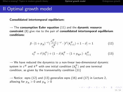
Consolidated intertemporal equilibrium:
→ The consumption Euler equation (11) and the dynamic resourceconstraint (8) give rise to the pair of consolidated intertemporal equilibriumconditions:
β · (1+ µA)−σ(
c#t+1c#t
)−σ · [f ′(k#t+1) + 1− δ] = 1 (12)
c#t = f (k#t ) + (1− δ)k#t − (1+ µN# ) · k
#t+1 (13)
→ We have reduced the dynamics to a non-linear two-dimensional dynamicsystem in c# and k# with one initial condition (k#0 ) and one terminalcondition, as given by the transversality condition (11)
→ Notice: eqns (12) and (13) generalize eqns (16) and (17) in Lecture 2,allowing for µA > 0 and µN > 0
19 / 54

What is missing? Topics in modern growth theory Optimal growth model Endogenous growth
II Optimal growth model
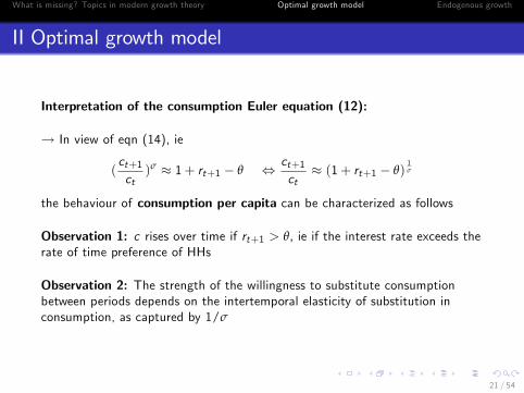
Interpretation of the consumption Euler equation (12):
→ How does consumption per capita (ie ct ) evolve over time?
Consider the consumption Euler equation (12), ie
β · (1+ µA)−σ(
c#t+1c#t
)−σ · [f ′(k#t+1) + 1− δ] = 1
Use c#t =ctAtand c#t+1 =
ct+1At+1
(which impliesc#t+1c#t
= ct+1ct
11+µA
) to see
that eqn (12)..:...satisfies in general the well-known structure
U ′(ct ) = βU ′(ct+1)[f′(k#t+1) + (1− δ)]
...can for the particular utility function assumed above be rewritten as,
(ct+1ct)σ =
f ′(k#t+1) + 1− δ
1+ θ≈ 1+ rt+1 − θ, (14)
using β = 11+θ and rt+1 = f ′(k#t+1)− δ.
20 / 54
What is missing? Topics in modern growth theory Optimal growth model Endogenous growth
II Optimal growth model
Interpretation of the consumption Euler equation (12):
→ In view of eqn (14), ie
(ct+1ct)σ ≈ 1+ rt+1 − θ ⇔ ct+1
ct≈ (1+ rt+1 − θ)
1σ
the behaviour of consumption per capita can be characterized as follows
Observation 1: c rises over time if rt+1 > θ, ie if the interest rate exceeds therate of time preference of HHs
Observation 2: The strength of the willingness to substitute consumptionbetween periods depends on the intertemporal elasticity of substitution inconsumption, as captured by 1/σ
21 / 54

What is missing? Topics in modern growth theory Optimal growth model Endogenous growth
II Optimal growth model
Steady states of the equation system (12) and (13):
In steady state the consumption Euler eqn (12) simplifies to
f ′(k#) + 1− δ =1β· (1+ µA)
σ = (1+ θ) · (1+ µA)σ ≈ 1+ θ + σµA ,
where the last step uses a first-order Taylor approximation around thevalues θ = µA = 0
In sum: steady states of the system (12) and (13) satisfy
f ′(k#) ≈ δ+ θ + σµA (15)
c# = f (k#)− (δ+ µN# ) · k# (16)
These two equations have a recursive structure and are solved by aunique steady state with solution values k#∗ and c#∗
22 / 54
What is missing? Topics in modern growth theory Optimal growth model Endogenous growth
II Optimal growth model
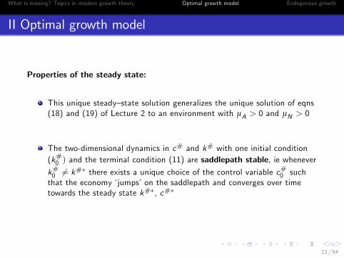
Properties of the steady state:
This unique steady—state solution generalizes the unique solution of eqns(18) and (19) of Lecture 2 to an environment with µA > 0 and µN > 0
The two-dimensional dynamics in c# and k# with one initial condition(k#0 ) and the terminal condition (11) are saddlepath stable, ie wheneverk#0 6= k#∗ there exists a unique choice of the control variable c
#0 such
that the economy ‘jumps’on the saddlepath and converges over timetowards the steady state k#∗, c#∗
23 / 54
What is missing? Topics in modern growth theory Optimal growth model Endogenous growth
II Optimal growth model
Similarities with the solution of the Solow-model:
Corresponding to the steady-state values c#∗ and k#∗ (which areexpressed in units of effective labour) there exists a unique balancedgrowth path. Along this path, per capita variables (ie kt , yt , ct , it ) growat the constant rate µA
Like in the Solow-model, the long-run growth rate of per capita variablesµA is exogenous, ie not explained from within the model
Like in the Solow-model, the implied differences in the per capita capitalstock and return rates on capital are implausibly large to explain outputper capita developments in a satisfactory manner
24 / 54

What is missing? Topics in modern growth theory Optimal growth model Endogenous growth
II Optimal growth model
Differences to the solution of the Solow-model:
The savings rate is (only) during the transition period towards the steadystate not constant
The steady-state value k#∗ is always smaller than the golden-rulelevel, ie
k#∗ < k#GR
Why? The assumed impatience of consumers implies that the long-runcapital stock is not high enough to support the maximum level ofsteady-state consumption
25 / 54
What is missing? Topics in modern growth theory Optimal growth model Endogenous growth
II Optimal growth model
Background: Establishing k#∗ < k#GR
→ Combine the golden-rule optimality criterion
f ′(k#GR ) = δ+ µN# ≈ δ+ µN + µA
and the optimality criterion (15) of the optimal growth model
f ′(k#∗) ≈ δ+ θ + σµA
to establish
k#∗ < k#GR ⇔ f ′(k#∗) > f ′(k#GR ) ⇔ θ − µN − (1− σ)µA > 0,
which is identical to the earlier imposed restriction (3)
26 / 54

What is missing? Topics in modern growth theory Optimal growth model Endogenous growth
II Optimal growth model
Background: Establishing k#∗ < k#GR
The restriction (3) can be linked to the transversality condition (9), ie
limt→∞
λt · k#t+1 = 0
which must always be satisfied
In particular, assume that k#t+1 and c#t converge against the optimal
long-run values k#∗ > 0, c#∗ > 0. Then, the TV-condition (9) will onlybe satisfied if
limt→∞
λt = 0
Recall from eqn (10) that λ grows according to
λtλt−1
= β · (1+ µN ) · (1+ µA)1−σ(
c#tc#t−1
)−σ,
which, using β = (1+ θ)−1, implies along a balanced growth path (withc#∗ being constant)
λtλt−1
=(1+ µN ) · (1+ µA)
1−σ
1+ θ27 / 54

What is missing? Topics in modern growth theory Optimal growth model Endogenous growth
II Optimal growth model
Background: Establishing k#∗ < k#GR
For limt→∞
λt = 0 we needλt
λt−1< 1, ie
λtλt−1
=(1+ µN ) · (1+ µA)
1−σ
1+ θ≈ 1+ µN + (1− σ) · µA − θ < 1,
which is equivalent to restriction (3), ie
θ − µN − (1− σ)µA > 0
In sum, for steady states to satisfy all optimality conditions therestriction (3) must hold. And this in turn implies k#∗ < k#GR
28 / 54

What is missing? Topics in modern growth theory Optimal growth model Endogenous growth
II Optimal growth model
Comments: Steady-state properties of the optimal growth model
1) Since it is optimal to converge against the value k#∗, this value is oftencalled the modified golden-rule capital stock
2) The resulting pattern ofk#∗ < k#GR
is called a constellation of dynamic effi ciency. Such constellation ischaracterized by the feature that a reduction of the long-run capital stock doesnot increase long-run consumption.
Notice: As discussed above, the steady state of the Solow-model (ie k#So ) is notnecessarily dynamically effi cient.
29 / 54

What is missing? Topics in modern growth theory Optimal growth model Endogenous growth
II Optimal growth model
Background: Relaxing the objective of the Benthamite welfare function
Assume one replaces the objective (1), ie V0 = ∑∞t=0 βtU(ct ) ·Nt ,
against the alternative objective ‘without population weights’, ie
V0 =∞
∑t=0
βtU(ct ) (17)
Notice that the objective (1) implied the effective discount factor
1+ µN1+ θ
≈ 1+ µN − θ
which under (17) will be replaced against the pure discount factor
β =1
1+ θ≈ 1− θ
The resulting stronger discounting under the alternative objective (17)implies that the long-run value of f ′(k#∗) will be higher, ie
f ′(k#∗) ≈ δ+ θ + µN + σµA ,
making the long-run value of the capital stock k#∗ smaller. Moreover,the modified condition (3) turns into
θ − (1− σ)µA > 0 30 / 54

What is missing? Topics in modern growth theory Optimal growth model Endogenous growth
III Endogenous growthAk-model
Let us consider the most simple model available which derives the percapita growth rate of the economy endogenously, the so-called Ak-modelof endogenous growth. The analysis goes back to Rebelo (1991)
Idea: we maintain the assumption of exogenous population growth(µN > 0), but there is no labour-augmenting technological progress
Crucial mechanism for long-run per capita growth of output,consumption, and capital: the production function is such that per capitaoutput is linear in capital
yt = A · kt , (18)
where A > δ+ θ > 0 is a constant (and the raw labour input aspreviously captured by nt is without return)
31 / 54
What is missing? Topics in modern growth theory Optimal growth model Endogenous growth
III Endogenous growthAk-model
Model ingredients:
Objective (identical to eqn (1)):
V0 =∞
∑t=0
βtU(ct ) ·Nt
We will use again the particular utility function U(ct ) =(ct )1−σ−11−σ , implying
V0 =∞
∑t=0
βt · (ct )1−σ − 11− σ
·Nt =∞
∑t=0[β · (1+ µN )]
t · (ct )1−σ − 11− σ
·N0 (19)
Dynamic constraint (per capita):
kt+1 · (1+ µN ) = A · kt − ct + (1− δ)kt , (20)
with the predetermined value k0 to be taken as given
32 / 54

What is missing? Topics in modern growth theory Optimal growth model Endogenous growth
III Endogenous growthAk-model
Can we expect per capita variables to grow over time or to be constant?
At this stage, we don’t know yet
→ If one solves the social planner’s problem in terms of per capita variables theconsolidated intertemporal equilibrium conditions look as follows:
Consumption Euler equation:
β · ( ct+1ct)−σ · [A+ 1− δ] = 1 (21)
Resource constraint:
kt+1 · (1+ µN ) = A · kt − ct + (1− δ)kt (22)
33 / 54

What is missing? Topics in modern growth theory Optimal growth model Endogenous growth
III Endogenous growthAk-model
Notice that the marginal product of capital (ie A) is constant
Hence, the consumption Euler equation, ie (21)
β · ( ct+1ct)−σ · [A+ 1− δ] = 1
can be used to establish the constant growth rate of per capita consumption(ie µ C
N)
ct+1ct
= 1+ µ CN= [β · (A+ 1− δ)]
1σ = [
A+ 1− δ
1+ θ]1σ ,
implying
ln(ct+1ct) =
1σ· ln(A+ 1− δ
1+ θ) ⇔ µ C
N≈ 1
σ· (A− δ− θ), (23)
where the approximation assumes that A, δ, and θ are numbers suffi cientlyclose to zero
34 / 54

What is missing? Topics in modern growth theory Optimal growth model Endogenous growth
III Endogenous growthAk-model
Interpretation of eqn (23), ie
µ CN≈ 1
σ· (A− δ− θ) ⇔ A− δ ≈ θ + σµ C
N
In the Ak-model long-run per capita growth is feasible even if oneassumes that there is no technological progress
Long-run growth is driven by the model feature that output moves inproportion to the capital stock. This is different from both the originalSolow-model and the optimal growth model, where it was assumed thatf (k) is subject to diminishing marginal productivity
As a result, in the Ak-model the growth rate of per capita consumptiondepends on a range of model parameters (ie σ, A, δ, θ)
Notice: The growth rate µ CNis independent of the starting position of the
economy (no transitional dynamics)
35 / 54

What is missing? Topics in modern growth theory Optimal growth model Endogenous growth
III Endogenous growthAk-model
Interpretation of eqn (23), ie
µ CN≈ 1
σ· (A− δ− θ) ⇔ A− δ ≈ θ + σµ C
N
→ How does in the Ak-model the growth rate of per capita consumptiondepend on model parameters ?
Example 1: If the productivity of capital (ie A) increases this leads to anincrease in µ C
NNotice: A is assumed to be exogenous in the model, but one can imagine thatpolicy interventions may have a chance to change A
Example 2: If consumers become more impatient (as captured by an increasein θ), this leads to a decline in µ C
N
Notice: Changes in θ are similar to changes in the savings behaviour. Inparticular, in the Solow-model, when combined with an Ak-technology, changesin s have long-run growth effects. Again, one can imagine that policyinterventions may have a chance to change s
36 / 54

What is missing? Topics in modern growth theory Optimal growth model Endogenous growth
III Endogenous growthAk-model
Comparison between exogenous and endogenous growth:
→ For comparison, it is instructive to see that the long-run solutions as givenby eqns (15) and (23) display a very similar structure:
f ′(k#∗)− δ ≈ θ + σ · µ CN︸︷︷︸
=µA
vs. f ′(k)︸ ︷︷ ︸=A
− δ ≈ θ + σ · µ CN
Exogenous growth:
The long-run per capita growth rate µ CNis uniquely fixed at the
exogenous rate µAChanges in θ and σ leave µ C
Nunaffected and induce changes in f ′(k#∗)
Endogenous growth (Ak model):
The marginal product of capital is uniquely fixed at the value A
Changes in θ and σ leave A unaffected and induce changes in theendogenous rate µ C
N
37 / 54
What is missing? Topics in modern growth theory Optimal growth model Endogenous growth
III Endogenous growthAk-model
Comparison between exogenous and endogenous growth:
→ These differences have significant implications for the quantitativepredictions of the models, like whether we should expect convergence of percapita incomes or not
Example: consider 2 countries with different attitudes towards intertemporalconsumption as captured by θ
→ Conditional convergence if long-run per capita growth is exogenous→ No convergence if long-run per capita growth is endogenous in the spiritof the Ak-model
Notice: Changes in θ are similar to changes in the savings behaviour. Inparticular, in the Solow-model, when combined with an Ak-technology, 2countries with different savings rates display different long-run growth rates, ieunder an Ak-technology there is no convergence (absolute or conditional) ofper capita incomes
38 / 54

What is missing? Topics in modern growth theory Optimal growth model Endogenous growth
III Endogenous growthAk-model
How should one read the Ak-model?
→ Essentially, the Ak-model offers a short-cut in reduced form which showsthat output can grow in proportion to capital if there exists some mechanismwhich offsets the standard assumption of diminishing private returns to physicalcapital
→ To conclude the lecture, we show that such mechanism - under twoalternative and more nuanced modelling approaches - can be made consistentwith:
1) the notion of constant returns to scale in the aggregate productionfunction with respect to physical capital and labour(→ Frankel, 1962, Romer, 1986)
2) the idea of a broad measure of capital which allows for both physical andhuman capital(→ Lucas, 1988)
39 / 54

What is missing? Topics in modern growth theory Optimal growth model Endogenous growth
III Endogenous growthRe-interpreting the Ak-model: externalities in capital accumulation
→ For many macroeconomic applications, a convenient starting point is theassumption of an aggregate production function in capital and labour of theCobb-Douglas-type, ie
Y = F (K ,N) = A ·K αNγ
To reconcile this assumption with the Ak-feature of a linear relationshipbetween output and capital is a priori not straightforward. Why?
→ The Ak-feature requires α = 1. This implies:
1) Labour can only play an active role (ie γ > 0) if one replaces the assumptionof constant returns to scale (‘CRTS’) in K and L against the assumption ofincreasing returns to scale (IRTS). But this is diffi cult to reconcile with theexistence of a competitive equilibrium in a decentralized environment in whichfirms maximize profits, taking factor prices of capital and labour as given
2) Conversely, the assumption of CRTS can only be maintained in thedegenerate scenario in which (raw) labour is entirely unproductive (γ = 0)
40 / 54

What is missing? Topics in modern growth theory Optimal growth model Endogenous growth
III Endogenous growthRe-interpreting the Ak-model: externalities in capital accumulation
Frankel (1962) and Romer (1986):
In general A stands for the knowledge embodied in the economy-widecapital stock...
...and the constancy of A may well capture appropriately sizedexternalities associated with the investment decisions of firms
→ The i) notion of CRTS in K and L in the aggregate production function andii) the Ak-feature of a linear relationship between capital and output can bereconciled
Idea:
individual firms perceive diminishing private returns to capital at the firmlevel
at the aggregate level, positive externalities of investment decisionsgenerate constant social returns to capital
all this is consistent with CRTS between labour and capital in theaggregate production function
41 / 54

What is missing? Topics in modern growth theory Optimal growth model Endogenous growth
III Endogenous growthRe-interpreting the Ak-model: externalities in capital accumulation
The main ingredients of Romer (1986) can be adapted to the above sketchedAk-model as follows:
Aggregate output is produced according to the technology:
Yt = At ·K αt N
1−αt ,
Per capita output:
yt =YtNt= At · kα
t
The variable At captures an externality which is a function of thecapital-labour ratio such that
At = A · kβt
Consider the special parameter case β = 1− α. Then, the externalityexactly offsets the diminishing private returns to capital induced by αsuch that per capita output becomes
yt = A · ktCrucial: the social planner solution internalizes the externality associatedwith At , differently from the solution provided by decentralized markets...
42 / 54
What is missing? Topics in modern growth theory Optimal growth model Endogenous growth
III Endogenous growthRe-interpreting the Ak-model: externalities in capital accumulation
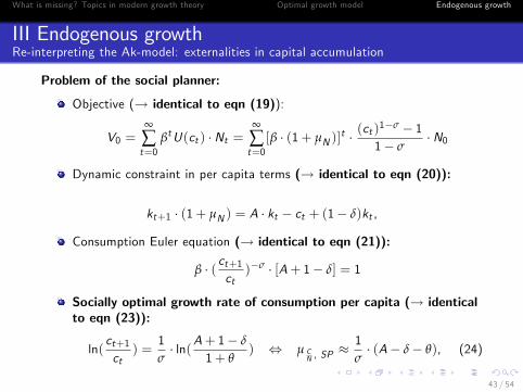
Problem of the social planner:
Objective (→ identical to eqn (19)):
V0 =∞
∑t=0
βtU(ct ) ·Nt =∞
∑t=0[β · (1+ µN )]
t · (ct )1−σ − 11− σ
·N0
Dynamic constraint in per capita terms (→ identical to eqn (20)):
kt+1 · (1+ µN ) = A · kt − ct + (1− δ)kt ,
Consumption Euler equation (→ identical to eqn (21)):
β · ( ct+1ct)−σ · [A+ 1− δ] = 1
Socially optimal growth rate of consumption per capita (→ identicalto eqn (23)):
ln(ct+1ct) =
1σ· ln(A+ 1− δ
1+ θ) ⇔ µ C
N , SP≈ 1
σ· (A− δ− θ), (24)
43 / 54

What is missing? Topics in modern growth theory Optimal growth model Endogenous growth
III Endogenous growthRe-interpreting the Ak-model: externalities in capital accumulation
Solution provided by decentralized markets:
→ Representative consumer/owner of the representative firm faces the samemaximization problem, but he or she takes as given the process At
Modified dynamic constraint in per capita terms (ie the representativefirm does not perceive a linear technology):
kt+1 · (1+ µN ) = At · kαt − ct + (1− δ)kt
Modified consumption Euler equation:
β · ( ct+1ct)−σ · [α · At · kα−1
t + 1− δ] = 1
The competitive equilibrium satisfies
At = A · k1−αt ,
implying for the consumption Euler equation
β · ( ct+1ct)−σ · [α · A+ 1− δ] = 1
44 / 54

What is missing? Topics in modern growth theory Optimal growth model Endogenous growth
III Endogenous growthRe-interpreting the Ak-model: externalities in capital accumulation
Solution provided by decentralized markets:
Thus, the growth rate of consumption per capita generated by thedecentralized market solution is given by
µ CN , MS
≈ 1σ· (α · A− δ− θ) (25)
Comparing (24) and (25) yields:
1σ· (α · A− δ− θ)︸ ︷︷ ︸
µ CN , MS
<1σ· (A− δ− θ)︸ ︷︷ ︸
µ CN , SP
Interpretation:
In the market solution individuals fail to internalize the effect of individualcapital accumulation on knowledge AtAs a result, the equilibrium growth rate of per capita variables is less thanthe socially optimal one
45 / 54

What is missing? Topics in modern growth theory Optimal growth model Endogenous growth
III Endogenous growthRe-interpreting the Ak-model: externalities in capital accumulation
Comment:
The process driving the externality At = A · kβt is a general one, while the
assumed parameter constellation
β = 1− α
which reproduces the Ak-model is very special
If one assumes, alternatively,
β < 1− α
per capita growth vanishes in the long run in the absence of exogenoustechnological progress (similar to the Solow model and the optimalgrowth model)
In sum, while this alternative assumption makes the long-run growthpredictions of the model close to the Solow model, the elasticity ofoutput with respect to (economy-wide) capital increases, improving onthe ability of Solow-type models, when augmented with externalities, topredict cross-country differences in Y
N via differences in KN
46 / 54

What is missing? Topics in modern growth theory Optimal growth model Endogenous growth
III Endogenous growthRe-interpreting the Ak-model: the role of human capital
→ A second and alternative mechanism to re-interpret the Ak-model as areduced form of a model with more compelling micro-foundations relates to theidea of a broad measure of capital which allows for separate contributionsto output from physical and human capital
→ For illustration, we consider a much simplified version of the model providedby Lucas (1988)
47 / 54

What is missing? Topics in modern growth theory Optimal growth model Endogenous growth
III Endogenous growthRe-interpreting the Ak-model: the role of human capital
Model ingredients:
We maintain the assumption of exogenous population growth (µN > 0),but there is no labour-augmenting technological progress
The production function has CRTS w.r.t. to the two inputs physicalcapital (K ) and human capital (H)(and raw labour N plays no role)
Per capita production function:
yt = A · kαt · h1−α
t with: α ∈ (0, 1)
Both types of capital subject to the same rate of depreciation δ ∈ (0, 1)
48 / 54

What is missing? Topics in modern growth theory Optimal growth model Endogenous growth
III Endogenous growthRe-interpreting the Ak-model: the role of human capital
Model ingredients:
Objective (→ identical to eqn (19)):
V0 =∞
∑t=0
βtU(ct ) ·Nt =∞
∑t=0[β · (1+ µN )]
t · (ct )1−σ − 11− σ
·N0
Dynamic constraint (per capita):
(kt+1 + ht+1) · (1+ µN ) = A · kαt · h1−α
t − ct + (1− δ)(kt + ht ),
with the predetermined values k0 and h0 to be taken as given
49 / 54
What is missing? Topics in modern growth theory Optimal growth model Endogenous growth
III Endogenous growthRe-interpreting the Ak-model: the role of human capital
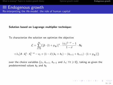
Solution based on Lagrange multiplier technique:
To characterize the solution we optimize the objective
L =∞
∑t=0{[β · (1+ µN )]
t · (ct )1−σ − 11− σ
·N0
+λt [A · kαt · h1−α
t − ct + (1− δ)(kt + ht )− (kt+1 + ht+1) · (1+ µN )]}
over the choice variables {ct , kt+1, ht+1 and λt ; ∀t > 0}, taking as given thepredetermined values k0 and h0
50 / 54

What is missing? Topics in modern growth theory Optimal growth model Endogenous growth
III Endogenous growthRe-interpreting the Ak-model: the role of human capital
L =∞
∑t=0{[β · (1+ µN )]
t · (ct )1−σ − 11− σ
·N0
+λt [A · kαt · h1−α
t − ct + (1− δ)(kt + ht )− (kt+1 + ht+1) · (1+ µN )]}
First-order optimality conditions (interior) w.r.t. ct , kt , ht and λt :
∂L∂ct
= [β · (1+ µN )]t ·N0 · (ct )−σ − λt = 0 t > 0
∂L∂kt
= λt [α · A · kα−1t · h1−α
t + 1− δ]− λt−1 · (1+ µN ) = 0 t > 0
∂L∂ht
= λt [(1− α) · A · kαt · h−α
t + 1− δ]− λt−1 · (1+ µN ) = 0 t > 0
∂L∂λt
= A · kαt · h1−α
t − ct + (1− δ)(kt + ht )
−(kt+1 + ht+1) · (1+ µN ) = 0 t > 0Transversality conditions: lim
t→∞λt · kt+1 = 0 and lim
t→∞λt · ht+1 = 0
51 / 54

What is missing? Topics in modern growth theory Optimal growth model Endogenous growth
III Endogenous growthRe-interpreting the Ak-model: the role of human capital
→ Because of the symmetric structure of the production function with respectto k and h, we get the pair of Euler equations:
β · ( ct+1ct)−σ · [α · A · kα−1
t+1 · h1−αt+1 + 1− δ] = 1
β · ( ct+1ct)−σ · [(1− α) · A · kα
t+1 · h−αt+1 + 1− δ] = 1
→ These two equations imply
kt+1ht+1
=kh=
α
1− α, (26)
ie the ratio between physical and human capital is constant
→ Thus, we can simplify the above pair of equations to the singleconsumption Euler equation
β · ( ct+1ct)−σ · [α · A · (k
h)α−1 + 1− δ] = 1 (27)
52 / 54

What is missing? Topics in modern growth theory Optimal growth model Endogenous growth
III Endogenous growthRe-interpreting the Ak-model: the role of human capital
Interpretation of the consumption Euler equation (27), ie:
β · ( ct+1ct)−σ · [α · A · ( k
h︸︷︷︸α1−α
)α−1 + 1− δ] = 1
Notice: since kh is constant, eqn (27) has a structure which is identical to
the consumption Euler eqn (21) of the Ak-model, ie capital is subject to aconstant marginal product along the optimal growth path (and there areno transitional dynamics)
This finding can also be seen from substituting (26) into the productionfunction
yt = A · kαt · h1−α
t = A · ( ktht)α−1 · kt = A · kt ,
ie we obtain the Ak-production function with
A = A · ( α
1− α)
α−1
53 / 54

What is missing? Topics in modern growth theory Optimal growth model Endogenous growth
III Endogenous growthRe-interpreting the Ak-model: the role of human capital
Interpretation of the consumption Euler equation (27), ie:
Accordingly, the growth rate of per capita consumption (µ CN) is
constant, ie
ct+1ct
= 1+ µ CN= [β · (α · A+ 1− δ)]
1σ = [
α · A+ 1− δ
1+ θ]1σ ,
implying
µ CN≈ 1
σ· (α · A− δ− θ),
where the approximation assumes that A, δ, and θ are numberssuffi ciently close to zero.
In sum: it is possible to re-interpret the Ak-model as a reduced form of amodel which allows for constant returns to scale to the 2 inputs physicalcapital and human capital
Comment: Lucas (1988) has a model which is richer. In particular, hismodel allows for externalities associated with the formation of humancapital. This implies that the solution of the social planner and thesolution provided by decentralized markets are not identical
54 / 54