lecture 5

Lecture 5The Capital Asset

Pricing Model,

Arbitrage Pricing Theory &

Cost of Capital

Financial Management(N12403)

Lecturer:

Farzad Javidanrad (Autumn 2014-2015)

Risk-Return Analysis

• In the previous lecture we talked about the risk associated to a security and how variance (or standard deviation) of returns of the security can measure this risk.

• We also mentioned that a rational investor hold a well diversified portfolio of different securities in order to reduce the level of unique (unsystematic, diversifiable) risk associated to individual securities, but market (systematic, non-diversifiable) risk cannot be eliminated.

• The idea that how diversification leads to the reduction of risk was formulated by Harry Markowitz in 1952 as he believed risk, as well as the highest expected return, is another element that investors care about and the variance of a portfolio does not only depend on the variance of individual assets in the portfolio but also on covariance between them.

• The risk of a portfolio is measured by its variance (or its standard deviation) but the risk of an individual asset (security) in the portfolio is measured by its covariance with other assets (securities) in the portfolio.

Risk-Return Analysis

• Imagine two portfolios A and B plotted based on their expected returns and their levels of risk (following diagrams). In each extreme case the best portfolio is:

A

B

Risk (Standard Deviation)

Expected Return %


Expected Return %

A B

A because it has more expected return at a specific level of risk

A because its risk is lower at a given level of return

𝜎𝐴 = 𝜎𝐵

𝑟𝐴

𝑟𝐵

𝑟𝐴 = 𝑟𝐵

𝜎𝐴 𝜎𝐵

Efficient Portfolios


• Now, suppose A is a portfolio with low risk and low return, compare to B with high return and high risk.

• If we imagine portfolios A and B have a perfect positive correlation (𝒓𝑨𝑩 = 𝟏) then there is a linear relationship between them (they are connected through the greenline) and any linear combination between them cannot bring the variance of the portfolio lower than the average of two variances. Therefore, it is not possible to reduce the risk by diversification.

Expected Return %

𝒓𝑨𝑩 = 𝟏

𝒓𝑨𝑩 < 𝟏

In reality, perfect positive correlation between two securities (𝒓𝑨𝑩 = 𝟏 ) does not exist.

when 𝒓𝑨𝑩 < 𝟏, diversification can reduce the level of risk and any combination under the red curve is feasible but a rational investor will find the best combination on the red curve and not below that. Why?

A

B

Efficient Portfolios

Expected Return %

𝒓𝑨𝑩 = 𝟏

𝒓𝑨𝑩 < 𝟏B

A

• The best portfolio is an efficient portfolio which gives the highest expected return at a given level of risk or lowest level of risk at a given expected return.

• Therefore, between portfolio A and C, a rational investor choose C as it gives the highest return at a certain level of risk.

• How can we find the best portfolios?

C


Portfolio with minimum risk

Efficient (Markovitz) Frontier

• In reality, we are facing with so many different portfolios not just two of them in our example.

• Let’s imagine that in the return-risk space we are dealing with portfolios, such as the following scatter plot, which shows a set of investment opportunities. Each point shows a portfolio which is a combination of different assets with different levels of risk and return. Obviously, the correlation should be positive. Why?

Expected Return % • At any level of expected return or at

any level of risk the green portfolios are the best. The curve which connects all the best portfolios at different levels of return & risk is called efficient frontier or Markovitzefficient frontier. So, the efficient frontier is the set of all efficient portfolios.


Risk-Return Indifference Curves

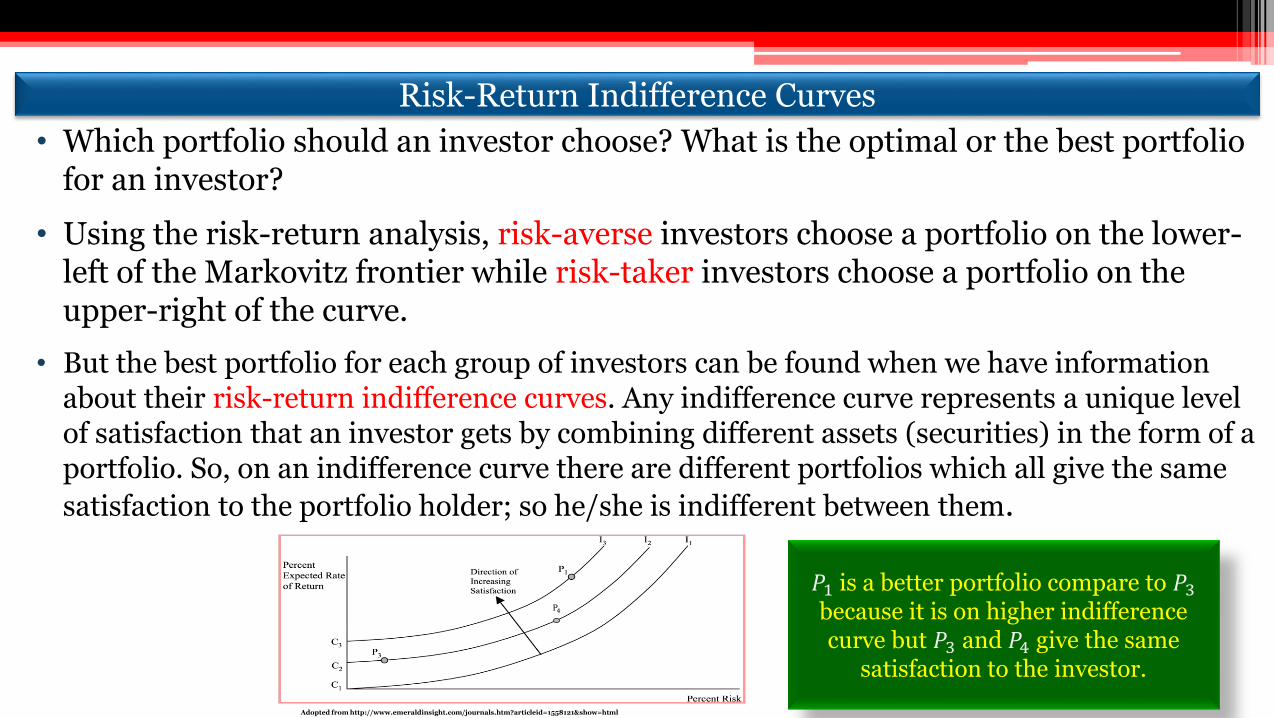
• Which portfolio should an investor choose? What is the optimal or the best portfolio for an investor?

• Using the risk-return analysis, risk-averse investors choose a portfolio on the lower-left of the Markovitz frontier while risk-taker investors choose a portfolio on the upper-right of the curve.

• But the best portfolio for each group of investors can be found when we have information about their risk-return indifference curves. Any indifference curve represents a unique level of satisfaction that an investor gets by combining different assets (securities) in the form of a portfolio. So, on an indifference curve there are different portfolios which all give the same

satisfaction to the portfolio holder; so he/she is indifferent between them.

Adopted from http://www.emeraldinsight.com/journals.htm?articleid=1558121&show=html

𝑃1 is a better portfolio compare to 𝑃3because it is on higher indifference curve but 𝑃3 and 𝑃4 give the same

satisfaction to the investor.

P4

Optimal Portfolio

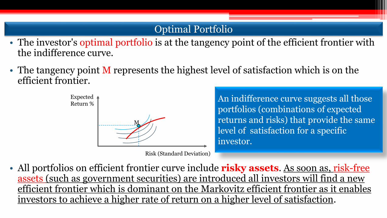
• The investor's optimal portfolio is at the tangency point of the efficient frontier with the indifference curve.

• The tangency point M represents the highest level of satisfaction which is on the efficient frontier.

• All portfolios on efficient frontier curve include risky assets. As soon as, risk-free assets (such as government securities) are introduced all investors will find a new efficient frontier which is dominant on the Markovitz efficient frontier as it enables investors to achieve a higher rate of return on a higher level of satisfaction.

Expected Return %


M

An indifference curve suggests all those portfolios (combinations of expected returns and risks) that provide the same level of satisfaction for a specific investor.

Introducing Risk-Free Assets

• Risk-free (risk-less) assets (such as government bonds, treasury bills) have some interesting characteristics, including:

1. Their expected return is equal to their actual return; 𝐸 𝑟𝑓 = 𝑟𝑓. This means that the

return from risk-free assets is with certainty.

2. For the above reason, the variance of their return is zero; 𝜎𝑟𝑓2 = 𝐸 𝑟𝑓 − 𝐸(𝑟𝑓)

2= 0.

3. The covariance between them and other risky assets are zero too; 𝑐𝑜𝑣 𝑟𝑓 , 𝑟 = 0.

• Combination of risk-free assets and risky assets provides higher level of return (at any specific level of risk) in compare with a portfolio of just risky assets.

• To show that, imagine an investor who is going to invest 𝜔 portion of his money on risky assets (for example, portfolio A on the efficient frontier) and the rest of that, (1 − 𝜔), on risk free assets.

Expected Return of a Portfolio Including Risk-Free Assets

• If 𝑟𝑓 is the return of risk-free assets and 𝐸(𝑟𝐴) is the expected return on the risky

portfolio A, the expected return and the standard deviation of the new combined

portfolio (𝐸 𝑟𝑝 and 𝜎𝑝) are:

𝐸 𝑟𝑝 = 𝝎𝐸(𝑟𝐴) + 𝟏 −𝝎 𝑟𝑓

And

𝜎𝑝 = 𝝎𝟐𝜎𝐴2 + 𝟏 −𝝎 𝟐𝜎𝑓

2 + 2𝝎 𝟏 −𝝎 𝑐𝑜𝑣(𝑟𝑓 , 𝐸(𝑟𝐴))

But we know that 𝜎𝑓2 = 0 and 𝑐𝑜𝑣 𝑟𝑓 , 𝐸(𝑟𝐴) = 0, therefore:

𝜎𝑝 = 𝝎𝜎𝐴 → 𝝎 =𝜎𝑝

𝜎𝐴Substituting this in we have:

𝐸 𝑟𝑝 =𝜎𝑝

𝜎𝐴𝐸(𝑟𝐴) + 1 −

𝜎𝑝

𝜎𝐴𝑟𝑓 → 𝐸 𝑟𝑝 = 𝑟𝑓 +

𝐸(𝑟𝐴) − 𝑟𝑓

𝜎𝐴𝜎𝑝

R

R

• The linear equation

𝐸 𝑟𝑝 = 𝑟𝑓 +𝐸(𝑟𝐴) − 𝑟𝑓

𝜎𝐴𝜎𝑝

is the risk-return trade-off between the expected return 𝐸 𝑟𝑝 and the risk 𝜎𝑝 for

efficient portfolios. The line is called the Capital Allocation Line (CAL).

• The intercept of the line is 𝑟𝑓, which is the point of risk-free rate on vertical axis and

the slope of the line is 𝐸(𝑟𝐴)−𝑟𝑓

𝜎𝐴, which is positive and reflects the fact

that higher risk

comes with higher

expected return.

Capital Allocation Line (CAL)

𝐸 𝑟𝑝

𝜎𝑝

𝑟𝑓

𝑪𝑨𝑳: 𝑬 𝒓𝒑 = 𝒓𝒇 +𝑬(𝒓𝑨) − 𝒓𝒇

𝝈𝑨𝝈𝒑

𝐴𝐸(𝑟𝐴)

Capital Market Line and Sharpe Ratio

• Any portfolio resulted from the combination of risk-free assets and risky portfolio A , i.e. any point on the line between 𝑟𝑓 and A , are superior to the points on the efficient frontier curve

and under the portfolio A, because the combination with free-risk assets provides a higher expected return.

• So, the new efficient frontier starts from 𝑟𝑓 to A and then continues on the previous Markovitz frontier.

𝐸 𝑟𝑝

A

𝑟𝑓𝜎𝑝

M

Portfolio A composed of only risky assets but a wise investor can buy some risk-free assets at rate 𝒓𝒇 to move

up on new efficient frontier, which introduce higher expected return. This new efficient frontier is called Capital Market Line (CML).

CML:

𝐸 𝑟𝑀

𝜎𝑀

𝐸 𝑟𝑝 = 𝑟𝑓 +𝐸(𝑟𝑀) − 𝑟𝑓

𝜎𝑀𝜎𝑝

Market price of risk= additional expected return that investors would require to compensate them for incurring additional risk.

Market Portfolio & Sharpe Ratio

• By taking more risks (moving along the efficient frontier) an investor can increase the expected return even higher and find better combinations like M.

• Point M is the tangency point and is the most efficient portfolio known as market portfolio as it is the most diversified portfolio and it includes just risky assets.

• This point also offers the highest slope that is; the highest ratio of risk premium to standard deviation which is called Sharpe ratio of the market portfolio.

Sharpe Ratio of (M)=𝐸(𝑟𝑀)−𝑟𝑓

𝜎𝑀

Alternatively, the Sharpe ratio of any portfolio 𝐴 (not on CML) can be written as:

𝑆ℎ𝑎𝑟𝑝𝑒 𝑅𝑎𝑡𝑖𝑜 𝑜𝑓 𝐴 =𝐸(𝑟𝐴)−𝑟𝑓

𝜎𝐴

Sharpe Ratio represents the excess return per unit

of risk

Borrowing/Lending at Risk-Free Rate

• All investors now have two jobs:

1. Finding the best portfolio (point M in our example)

2. Lend or borrow in order to reach to a suitable risk level they can bear in which higher expected return is embedded.

M

𝑟𝑓

𝐸 𝑟𝑝

𝐸 𝑟𝑀

𝜎𝑀

• With the lending/borrowing opportunity at the risk-free rate, an investor is no longer restricted to holding a portfolio on the efficient frontier.

• They can now invest in combinations of risky and risk-free assets in accordance with their risk preferences.

• A risk-averse investor will put part of their money in the efficient portfolio M and part of that in the risk-free assets. A risk-taker investor may put all their money in the best portfolio M or may even borrow and invest all of them on M.

𝑪𝑴𝑳: 𝑬 𝒓𝒑 = 𝒓𝒇 +𝑬(𝒓𝑴) − 𝒓𝒇

𝝈𝑴𝝈𝒑

Borrowing/Lending in the Absence of Risk-Free Rate

• When risk-averse investors buy risk-free assets such as government securities at rate 𝑟𝑓, in fact, they lend their money to the government. So, the efficient frontier line

before the point M (the line between 𝑟𝑓 and M) is called lending portfolio as it

includes a portion (1 − 𝜔) of the government securities.

• In case, that risk-taker investors are able to borrow at the same rate (𝑟𝑓), in order to

invest more at point M, the efficient frontier after M is called borrowing portfolio. But in reality, risk-taker investors are not able to find such a good rate to borrow and need to accept higher rates of borrowing (such as 𝑟𝑏). Therefore, the efficient frontier will be different:

M

B

𝐸 𝑟𝑝

𝜎𝑝𝑟𝑓

𝑟𝑏

Z

New efficient frontier when there is two different rates of

borrowing/lending:𝑟𝑓𝑀𝐵𝑍

The Capital Asset Pricing Model (CAPM)

• Capital market line introduces efficient portfolios but does not say anything about the relationship between expected return and risk for individual assets or even inefficient portfolios.

• The capital asset pricing model (CAPM) is a linear relationship between the expected rate of return of an individual asset (which is going to be added to an already well-diversified portfolio) and its contribution to the portfolio’s risk.

• CAPM is a model for pricing an individual asset 𝑖 by connecting its expected rate of return (𝐸(𝑟𝑖)) to the risk-free rate of interest (𝑟𝑓), expected return on

market portfolio (𝐸 𝑟𝑚 ), the variance of the return on the market portfolio (𝜎𝑚2 ) and the risk contributed to the portfolio by the risky asset (𝑐𝑜𝑣 𝑟𝑖 , 𝑟𝑚 =𝜎𝑖𝑚 = 𝜌𝜎𝑖𝜎𝑚).

The Capital Asset Pricing Model (CAPM)

• The idea behind pricing is that no individual security should be over-valued or under-valued in compare to the market values. So, the reward-to-risk ratio for an individual risky asset should be equal to the reward-to-risk ratio of the overall market; i.e.

𝐸 𝑟𝑖 −𝑟𝑓

𝜎𝑖𝑚=𝐸 𝑟𝑚 −𝑟𝑓

𝜎𝑚2

Where risk here is expressed in terms of the variance and not standard deviation.

• By re-writing equation and make 𝐸 𝑟𝑖 as the subject, we have:

𝐸 𝑟𝑖 = 𝑟𝑓 + (𝐸 𝑟𝑚 − 𝑟𝑓) ×𝜎𝑖𝑚

𝜎𝑚2

= 𝑟𝑓 + (𝐸 𝑟𝑚 − 𝑟𝑓) × 𝛽

Where 𝛽 measures the sensitivity of the asset to the market movements and it is representative of the systematic (market) risk.

Q

Q

Market Premium

Risk Premium

Security Market Line

• The re-written form of the equation is called Security Market Line (SML), which shows the relation between the expected return of an asset and its systematic risk 𝛽.

• SML states that individual risk premium is equal to market premium times the systematic risk 𝛽 and it is a useful tool in determining whether an individual asset offers a rational expected return for the risk contributed to the whole portfolio.

Q

Adopted from http://en.wikipedia.org/wiki/File:SML-chart.png

Securities with 𝜷>𝟏 amplify the overall movements of the market; with 0<𝜷<𝟏 theymove in the same direction as the market but slower than the market. Finally securities with 𝜷=𝟏 or close to that represent the market portfolio.

0.5 2

SML: 𝑬 𝒓𝒊 = 𝒓𝒇 + 𝑬 𝒓𝒎 − 𝒓𝒇 . 𝜷

Security Market Line

• Individual assets are plotted on the SML graph. If they are plotted above the SML, they are undervalued because the investor can expect a greater returns compare to their risks. A assets plotted below the SML are overvalued as the investor would think their prices are too high compare to alternative assets with higher return at the same level of risk.

• In a competitive market where all investors have the same information and knowledge about risk and returns of all assets, price of overvalued or undervalued assets moves to the equilibrium level on the SML line.

• CAPM provides a method of pricing an asset (such as a bond) based on our knowledge about the systematic risk 𝛽 and the expected rate of return in the market. So, we can write:

𝑃𝑉 =

𝑖=1

𝑛𝐶𝑖

1 + 𝑟𝑓 + 𝛽. 𝐸 𝑟𝑚 − 𝑟𝑓𝑖

𝑬 𝒓𝒊

Comparing CML & SML

• The Capital Market Line (CML) shows the expected rates of return for efficient portfolios as a function of the risk (standard deviation) of returns. CML cannot be adopted for individual assets and the measure of risk is the standard deviation of the market portfolio 𝜎𝑀.

• The Security Market Line (SML) can be applied both for individual assets and efficient portfolios. It gives the required rate of return on an asset (security) as a function of its contribution risk to the total risk of portfolio (𝛽). Practically, this relation can be used as a point of reference to determine the equilibrium level of expected return of a risky asset.

Assumption Behind CAPM

1. There is a risk-free securities and there expected returns are the real returns with zero risk. But in reality there is no guarantee for this assumptions.

2. Same lending and borrowing rates. But generally borrowing rate is higher than lending rate and for some risky investments the rate is even much higher compare to less-risky investments.

3. All investors behave rationally and have the same knowledge about the market portfolio and the risk of the market portfolio is known. Acquiring the knowledge is free and they do not need to pay to gain that.

4. Investors have identical preferences and homogeneous expectations.

5. All investors know how to calculate and measure the market return.

6. No taxes and no inflation. In fact, there is no government or an intermediary to bring imperfections into the market by imposing taxes, regulations or any specific of franchise or restriction.

Arbitrage Pricing Theory (APT)

• Some of these assumptions of CAPM seems to be unrealistic. (can you identify them?)

• There is another approach to asset pricing called Arbitrage Pricing Theory(APT), which was developed by Stephen Ross in 1976. APT uses a linear statistical model in contrary with CAPM, which uses comparative static model based on equilibrium analysis.

• The APT does not concentrate on efficient portfolios and assumes that stock’s return could be affected by many unanticipated changes in financial and economic factors and the systematic risk can be measured by many macroeconomics factors but the theory does not specify any superior or distinct factor and it also does not specify number of the factors.


• The APT relies on the absence of free arbitrage opportunities, which means no investor can take advantage of price difference of stocks in different markets.

• Two portfolios with the same level of risk cannot offer different expected returns, because that would present an arbitrage opportunity (benefiting from price difference without investing on anything).

• There are three major assumptions in APT:

1. Capital markets are perfectly competitive.

2. Investors always prefer more wealth to less wealth with certainty.

3. The stochastic process generating asset returns can be expressed as a linear function of a set of K factors or indexes.


• Possible factors may include particular sector-specific influences, such as price-dividend ratios, as well as aggregate macroeconomic variables such as inflation and interest rate spreads. (D.N. Tambakis, 2000, p 2)

• According to APT the return of a stock can be written as:

𝑟 = 𝛼 + 𝛽1𝐹1 + 𝛽2𝐹2 +⋯+ 𝛽𝑘𝐹𝑘 + 𝑢

Where

𝑟=Asset return

𝛽𝑗=Sensitivity of asset return to factor j

𝐹𝑗=Factor j

𝑢=Disturbance (error) term (some variables that cannot be measured but affecting 𝑟either positively or negatively)


• The factors 𝐹𝑗 need not necessarily be returns on an index or asset group; they

can be time-series observations of variables (e.g. interest rates, yield spreads, inflation (CPI) or other macroeconomic time series) which are thought to have an influence on the assets’ returns.

• The factors need not have zero mean, but they should always have zero covariance with the error terms, reflecting their definition as sources of systematic risk, and that of errors as sources of unsystematic (diversifiable) risk. ( D.N. Tambakis, 2000, p 3)


• For simplicity, imagine that the factors 𝐹𝑗 represent returns on group of assets then the expected risk premium on a stock should depend on the expected risk premium associated to each factor and the sensitivity of the return to each factor; i.e.

𝐸𝑥𝑝𝑒𝑐𝑡𝑒𝑑 𝑟𝑖𝑠𝑘 𝑝𝑟𝑒𝑚𝑖𝑢𝑚 = 𝑟 − 𝑟𝑓 = 𝛽1 𝑟𝐹1 − 𝑟𝑓 + 𝛽2 𝑟𝐹2 − 𝑟𝑓 +⋯+ 𝛽𝑘 𝑟𝐹𝑘 − 𝑟𝑓

• Fama and French have suggested three factors:

The return on market portfolio The difference between returns of small and large –firm stocks The difference between the return on stocks with high book-to-market ratio and

stocks with low book-to-market ratio

CAPM vs APT

• So far, we have focused on CAPM and APT models. Although their approaches are different but both of them argue that the expected return of a security (i.e. the appropriate discount rate for its PV of cash flows, which represents the price of the security) is a linear function of systematic or market risk.

• The main difference between CAPM and APT is that the CAPM uses one variable for risk, which is the market portfolio, but the APT employs different and more typically macroeconomic factors. These macro-variables affect the market portfolio. Thus, the single factor, market portfolio, in CAPM can be considered as a resultant of multi-factor variations in the APT.

• Also in the previous chapter we learnt that 𝛽 represents the market (systematic) risk and this risk can be a good representative of the level of existing risk in the whole economy. For this reason, systematic risk 𝛽 is also known as business cycle risk.

Beta ( A Risk Measure For Assets & Companies)

• Stocks that lose their values dramatically when the financial market falls are those with high betas. Stocks with low beta move in the same direction that market moves but their movement is slower.

• Even companies with high level 𝛽 (such as companies who work in high technology industry) are more vulnerable to the business cycles or financial instabilities in the economy in compare to companies with low level 𝛽 (such as companies who work in food industry), but if they survive the fall they can come up quickly.

• Estimating the beta of a company’s stock is important as it allows the financial manager of the company have an idea about the expected return on all the company’s securities, which is called company cost of capital that will be introduced later.

Finding Beta

• One way to estimate 𝛽 of a company (or a security) is to plot the company’s (security’s) returns, on y-axis, against the market returns, on x-axis in a specific period of time and estimate the regression line (line of best fit). The slope of this line is an estimation of 𝛽, which shows the magnitude of the change of company’s (security’s) returns to the change in market returns.

• Note that 𝛽 may change during the time due to changes in the market or in the investment strategy of the company.

• Knowing 𝛽 helps us to find company cost of capital, which is the next topic.Adopted from http://seekingalpha.com/article/241113-regression-to-the-moon-turning-nonsense-into-numbers

Adopted from http://mosaic.cnfolio.com/M591CW2008A101

Company Cost of Capital

• What discount rate a company should use to evaluate the PV of different investment projects?

• If we believe most companies show a stable behaviour in accepting certain level of risk in their overall activities; so, the company cost of capital, which is a risk-adjusted discount rate, can be used as a benchmark.

• So; for a company

𝑜𝑝𝑝𝑜𝑟𝑡𝑢𝑛𝑖𝑡𝑦 𝑐𝑜𝑠𝑡 𝑜𝑓 𝑐𝑎𝑝𝑖𝑡𝑎𝑙 > 𝑐𝑜𝑚𝑝𝑎𝑛𝑦 𝑐𝑜𝑠𝑡 𝑜𝑓 𝑐𝑎𝑝𝑖𝑡𝑎𝑙 ↔ 𝑃𝑟𝑜𝑗𝑒𝑐𝑡 𝑖𝑠 𝑟𝑖𝑠𝑘𝑦𝑜𝑝𝑝𝑜𝑟𝑡𝑢𝑛𝑖𝑡𝑦 𝑐𝑜𝑠𝑡 𝑜𝑓 𝑐𝑎𝑝𝑖𝑡𝑎𝑙 < 𝑐𝑜𝑚𝑝𝑎𝑛𝑦 𝑐𝑜𝑠𝑡 𝑜𝑓 𝑐𝑎𝑝𝑖𝑡𝑎𝑙 ↔ 𝑃𝑟𝑜𝑗𝑒𝑐𝑡 𝑖𝑠 𝑛𝑜𝑡 𝑟𝑖𝑠𝑘𝑦

• But how can we find the company cost of capital?

• The company cost of capital is defined as the expected return on a portfolio of all the company’s existing securities. It is the opportunity cost of capital for investment in the firm’s assets and therefore [it is] the appropriate discount rate for the firm’s average-risk projects. (Barely et.al , p 219)

Company Cost of Capital (With No Debt)

• If a company has no outstanding debt and the risk of a project is not much deviated from the firm’s existing projects, then the company’s cost of equity,which is obtained from the security market line (SML) is:

𝑟𝐸 = 𝑟𝑓 + 𝛽𝐸 . 𝑟𝑚 − 𝑟𝑓

But working with the above formula requires a knowledge about company’s equity 𝛽𝐸, which we discussed earlier. For example, if 𝑟𝑓 = 1.5% and the market risk

premium 𝐸 𝑟𝑚 − 𝑟𝑓 is about 8% and asset beta for a company is 𝛽𝐸 = 0.8, then the

expected return on equities for the company will be:

𝑟𝐸 = 1.5 + 0.8 × 8 = 7.9%

So, for a risky project the company should accept to invest on it if the rate of return from the project is above this rate.


• Graphically, this means any risky projects that lie above the 7.9% horizontal line (company cost of capital) can be accepted.

Adopted and amended from http://viking.som.yale.edu/will/finman540/classnotes/class7.html

7.9%

0.8

𝑟𝐸 = 𝑟𝑓 + 𝛽𝐸 . 𝑟𝑚 − 𝑟𝑓

Security Market Line (SML) shows

the required return on project

When there is no debt the company cost of capital is measured by the company’s cost of equity. In this example, 7.9% is the return on equity (cost of equity) but at the same time (as a fixed value) it is the company cost of capital.

Company cost of capital with no debt

Company Cost of Capital (With Debt)

• But this rate is not very realistic because the assumption of having no outstanding debt (specifically for large corporations) is far from the reality.

• A portfolio of all company’s securities (which expected return on that is the company cost of capital) includes debt as well as equity.

• According to the balance sheet of any company, the company’s market value 𝑉 (= asset value of the company in the market) is the summation of the company’s debt 𝐷 and the company’s equity 𝐸, i.e.

𝑉 = 𝐷 + 𝐸

• The company cost of capital, in this case, is not the cost of debt or the cost of equity but it is a weighted average cost of capital (average rate of returns demanded by investors) that the company acquired through debt or equity.


• Therefore, if the interest rate paid to the lenders is shown by 𝑟𝐷 and the rate of return to equity holders can be shown by 𝑟𝐸, the company cost of capital is: (remember that 𝑟𝐷is always lower than 𝑟𝐸)

𝑪𝒐𝒎𝒑𝒂𝒏𝒚 𝒄𝒐𝒔𝒕 𝒐𝒇 𝒄𝒂𝒑𝒊𝒕𝒂𝒍 = 𝒓𝑫 .𝑫

𝑽+ 𝒓𝑬 .

𝑬

𝑽Which is the weighted average cost of capital for a company and is usually called WACC. For example, for a company with a balance sheet composed of 40% debt and 60% equity, if 𝑟𝐷and 𝑟𝐸 are 8% and 12% respectively, then the company cost of capital will be:

𝐶𝑜𝑚𝑝𝑎𝑛𝑦 𝑐𝑜𝑠𝑡 𝑜𝑓 𝑐𝑎𝑝𝑖𝑡𝑎𝑙(𝑊𝐴𝐶𝐶) = 8 × 0.4 + 12 × 0.6 = 10.4%

• To be even closer to the reality we need to deduct tax imposed by government on any interests paid to lenders and this is part of the corporation’s expenses. So, after-tax cost of debt is 1 − 𝑇 . 𝑟𝐷 and eventually after-tax WACC can be calculated by:

𝐀𝐟𝐭𝐞𝐫 − 𝐭𝐚𝐱 𝐖𝐀𝐂𝐂 = (𝟏 − 𝑻)𝒓𝑫 .𝑫

𝑽+ 𝒓𝑬 .

𝑬

𝑽

Asset Beta

• Similarly, the company’s beta (company’s asset beta) can be calculated as:

𝛽𝑎𝑠𝑠𝑒𝑡 = 𝛽𝐴 = 𝛽𝐷 .𝐷

𝑉+ 𝛽𝐸 .𝐸

𝑉

• This asset beta is an estimate of the average risk of the company and it is used as a benchmark. If the investment ground is completely new this benchmark does not exist.

• What determines asset betas?

I. Cyclicality: Cyclical businesses such as luxury resorts, constructions, hotels and restaurants have a cyclical revenues depending on the state of the business cycle. These companies have high level of beta compare to businesses such as supermarkets and utility companies.

Asset Beta

II. Operating Leverage: For a company with a high fixed cost comparing to its variable cost the operating leverage is high and this means that the asset beta for such company is high.

III. Other Sources of Risk: Any change in the state of economy or state of confidence, which has an impact on the risk-free rate 𝑟𝑓 or the market risk premium 𝑟𝑚 − 𝑟𝑓, will change the

risk-adjusted discount rate 𝑟 used in discounting the expected cash flows in the project’s PV. Also a very long-term cash-flows can be considered as another source of risk.

• Forward-looking managers always take variety factors into account in their decisions. Existence of uncertainty in the economy is always a major

lecture 5

Education