Mauricio Lopes – FNAL

Lecture 4: Magnet Excitation and Coil

Design

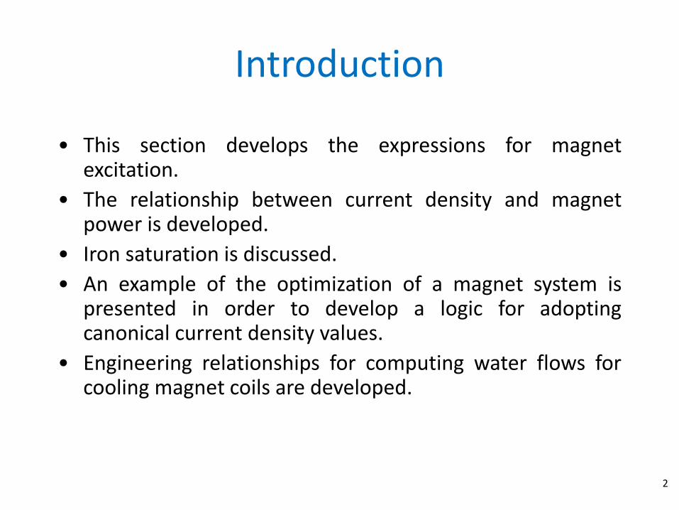
Introduction

2

• This section develops the expressions for magnet excitation.

• The relationship between current density and magnet power is developed.

• Iron saturation is discussed.

• An example of the optimization of a magnet system is presented in order to develop a logic for adopting canonical current density values.

• Engineering relationships for computing water flows for cooling magnet coils are developed.

Maxwell’s Equations (in media)

𝛻.𝑫 = 𝜌𝑓

𝛻.𝑩 = 0

𝛻 × 𝑬 = −𝜕𝑩

𝜕𝑡

𝛻 × 𝑯 = 𝑱𝒇 + 𝜕𝑫

𝜕𝑡

Gauss’s law

Faraday’s law

Ampere’s law

𝑫.𝑑𝑨 = 𝑄𝑓

𝑩. 𝑑𝑨 = 0

𝑬. 𝑑𝒍 = − 𝜕𝑩

𝜕𝑡. 𝑑𝑨

𝑯. 𝑑𝒍 = 𝑰𝒇 + 𝜕𝑫

𝜕𝑡. 𝑑𝑨

3

Ampere’s Law - Integral Form

4

𝑯.𝑑𝒍 = 𝐼𝑇

𝑯 =𝑩

𝜇𝑜. 𝜇𝑟 𝐼𝑇 = 𝑁𝐼 𝜇𝑜 = 4𝜋. 10

−7

𝜇𝑟_𝑎𝑖𝑟 = 1

𝜇𝑟_𝐼𝑟𝑜𝑛 ≈ 1000∗

𝑁 = Number of turns

𝐼 = Current

𝐼𝑇 = Total current

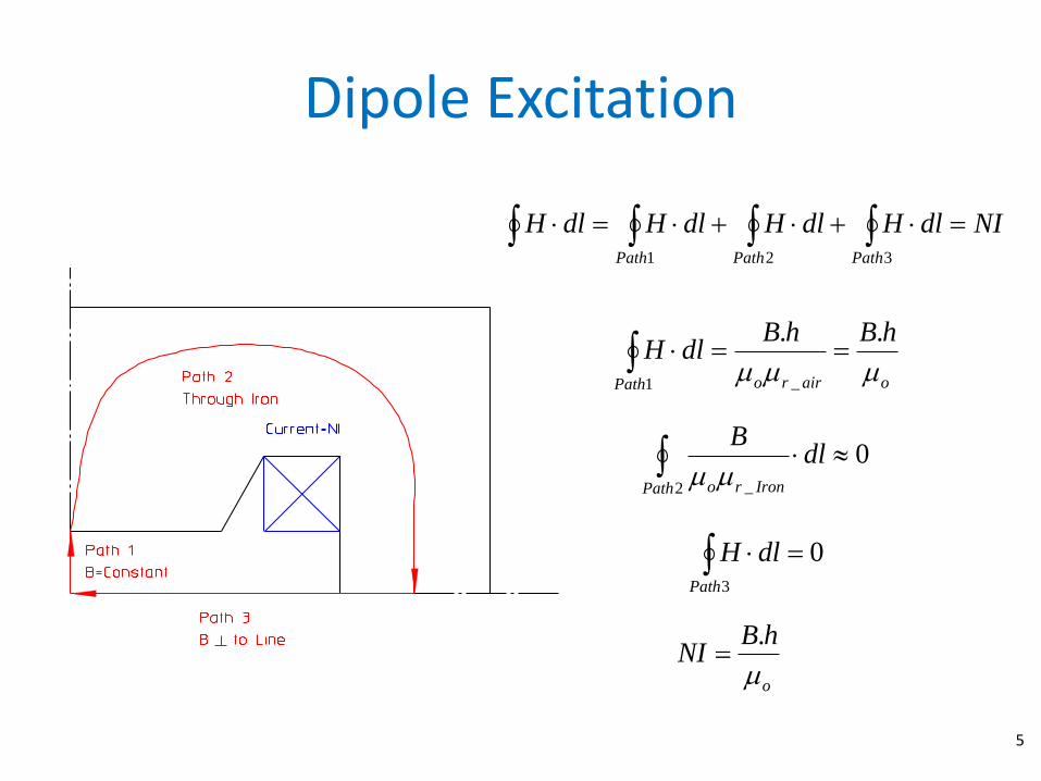
Dipole Excitation

NIdlHdlHdlHdlHPathPathPath

321

02 _

Path Ironro

dlB

oairroPath

hBhBdlH

..

_1

03

Path

dlH

o

hBNI

.

5

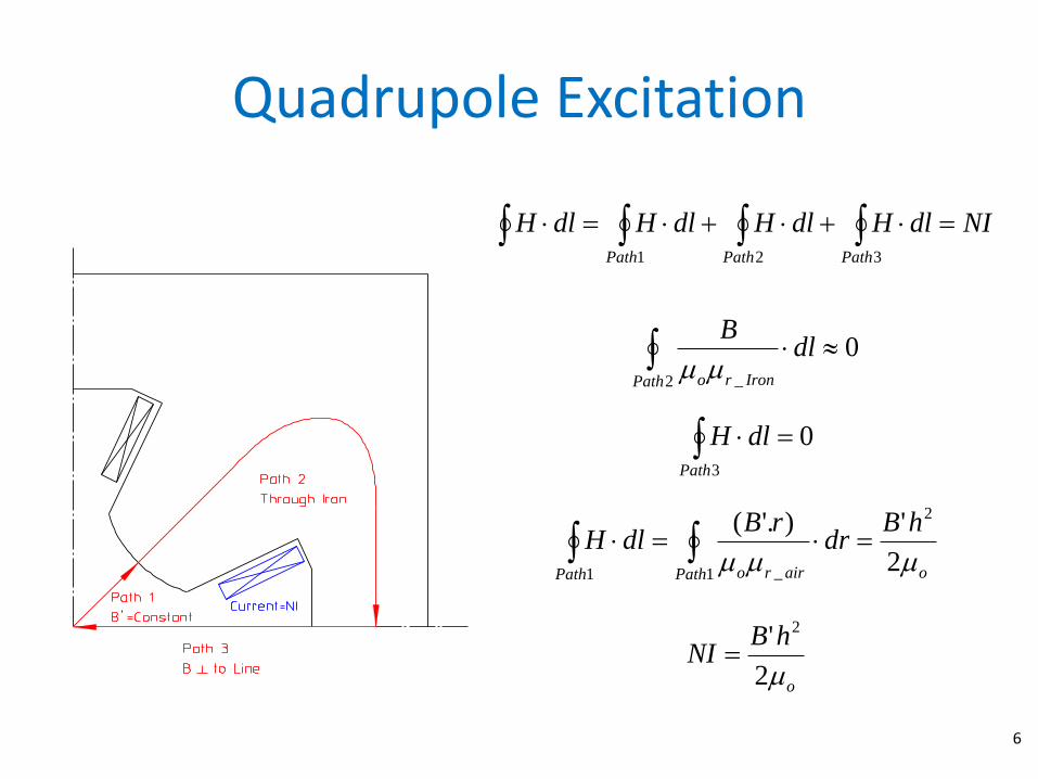
Quadrupole Excitation

NIdlHdlHdlHdlHPathPathPath

321

02 _

Path Ironro

dlB

oPath airroPath

hBdr

rBdlH

2

')'.( 2

1 _1

03

Path

dlH

o

hBNI

2

' 2

6

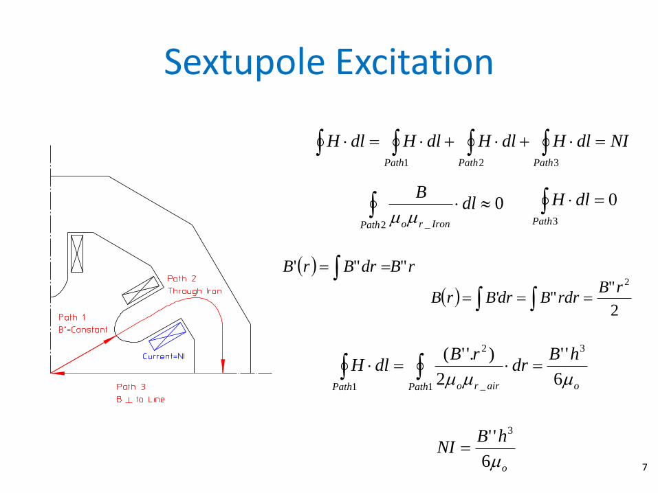
Sextupole Excitation

NIdlHdlHdlHdlHPathPathPath

321

02 _

Path Ironro

dlB

oPath airroPath

hBdr

rBdlH

6

''

2

)'.'( 3

1 _

2

1

03

Path

dlH

o

hBNI

6

'' 3

rBdrBrB ""'

2

""'

2rBdrrBdrBrB

7

B-H Curve

8

0

200

400

600

800

1000

1200

1400

1600

1800

2000

0.0

0.5

1.0

1.5

2.0

2.5

0 1000 2000 3000 4000 5000 6000 7000 8000 9000 10000

μr

B (

T)

H (A/m)

B (T)

μr

Magnet Efficiency

We introduce efficiency as a means of describing the losses in the iron. USe the expression for the dipole excitation as an example.

321 PathPathPath

dlHdlHdlHNI

00

1

BhBhfactorsmallNI

98.0 efficiency For magnets with well designed yokes.

lB

Bhfactorsmall

Bh

PathPathPath

since0

321

00

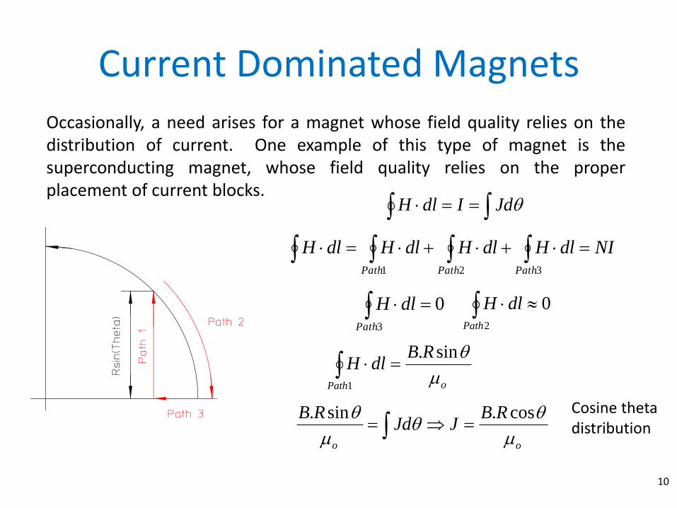
Current Dominated Magnets

10

Occasionally, a need arises for a magnet whose field quality relies on the distribution of current. One example of this type of magnet is the superconducting magnet, whose field quality relies on the proper placement of current blocks.

JdIdlH

NIdlHdlHdlHdlHPathPathPath

321

03

Path

dlH 02

Path

dlH

oPath

RBdlH

sin.

1

oo

RBJJd

RB

cos.sin.

Cosine theta distribution

Cosine Theta Current Distribution

11

Current Density

• One of the design choices made in the design of magnet coils is the choice of the coil cross section which determines the current density.

• Given the required Physics parameters of the magnet, the choice of the current density will determine the required magnet power.

– Power is important because they affect both the cost of power supplies, power distribution (cables) and operating costs.

– Power is also important because it affects the installation and operating costs of cooling systems.

12

Canonical Current Densities

13

AWG Diameter

(mm) Area

(mm2) r (W/km)

Max Current (A)

Max Current Density (A/mm2)

1 7.348 42.4 0.406392 119 2.81

2 6.543 33.6 0.512664 94 2.80

3 5.827 26.7 0.64616 75 2.81

…

…

…

…

…

…

38 0.102 0.00797 2163 0.0228 2.86

39 0.089 0.00632 2728 0.0175 2.77

40 0.079 0.00501 3440 0.0137 2.73

~ 10 A/mm2

Solid conductor

Hollow conductor

(with proper cooling)

RIPPower 2

)(m area sectional crossnet conductor =a

(m)length conductor =L

m)-(Ωy resistivit=

where

2

rr

a

LR

Coil main parameters

14

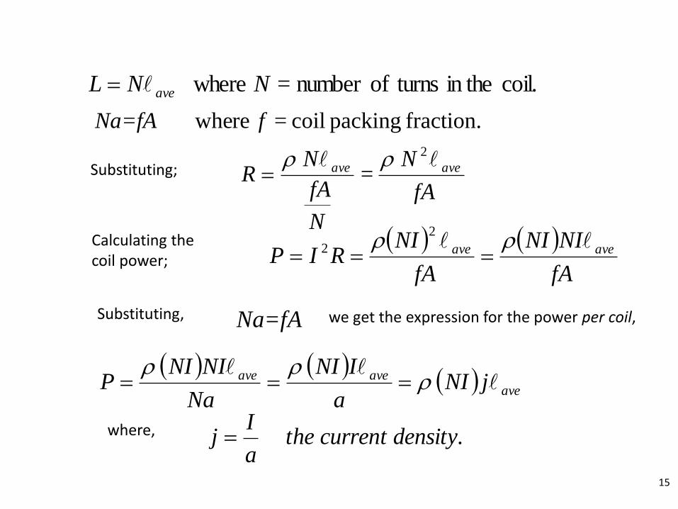
coil. in the turnsofnumber = where NNL ave

fraction. packing coil = re whe fNa=fA

fA

N

N

fA

NR aveave 2

= rr

Substituting;

fA

NINI

fA

NIRIP aveave rr

2

2Calculating the coil power;

Na=fA

ave

aveave jNIa

INI

Na

NINIP

r

rr

Substituting, we get the expression for the power per coil,

. t densitythe currena

Ij where,

15

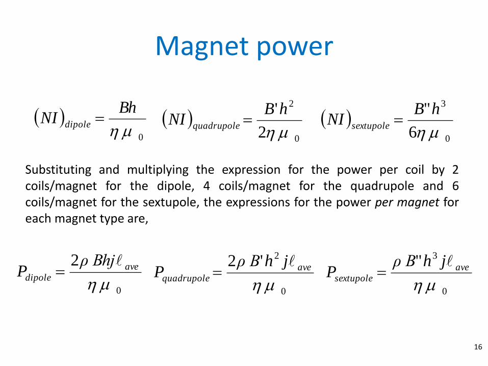
0

3

6

"

hBNI sextupole

0

2

2

'

hBNI quadrupole

0

BhNI dipole

0

2

ave

dipole

ρ BhjP

0

2

'2

ave

quadrupole

jhρ BP

0

3

"

ave

sextupole

jhρ BP

Substituting and multiplying the expression for the power per coil by 2 coils/magnet for the dipole, 4 coils/magnet for the quadrupole and 6 coils/magnet for the sextupole, the expressions for the power per magnet for each magnet type are,

Magnet power

16

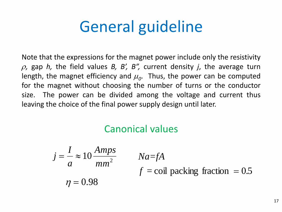
Note that the expressions for the magnet power include only the resistivity r, gap h, the field values B, B’, B”, current density j, the average turn length, the magnet efficiency and 0. Thus, the power can be computed for the magnet without choosing the number of turns or the conductor size. The power can be divided among the voltage and current thus leaving the choice of the final power supply design until later.

210

mm

Amps

a

Ij

98.050fraction packing coil =

.f

Na=fA

17

General guideline

Canonical values

Magnet System Design

• Magnets and their infrastructure represent a major cost of accelerator systems since they are so numerous.

• Magnet support infrastructure include:

Power Supplies

Power Distribution

Cooling Systems

Control Systems

Safety Systems

18

Power Supplies

19

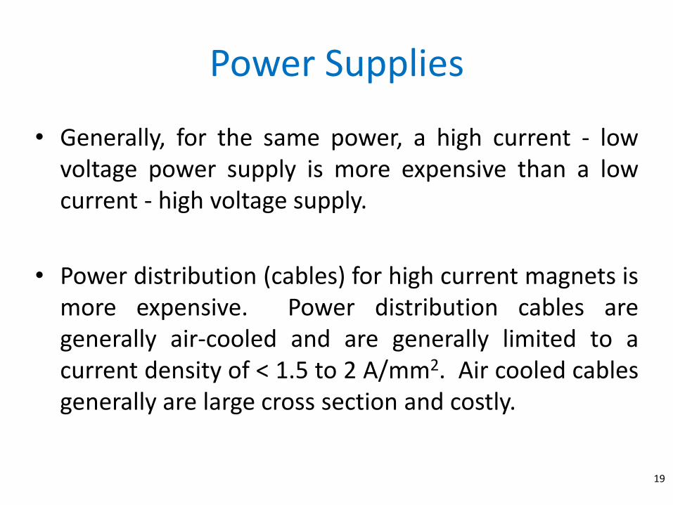
• Generally, for the same power, a high current - low voltage power supply is more expensive than a low current - high voltage supply.

• Power distribution (cables) for high current magnets is more expensive. Power distribution cables are generally air-cooled and are generally limited to a current density of < 1.5 to 2 A/mm2. Air cooled cables generally are large cross section and costly.

Dipole Power Supplies

20

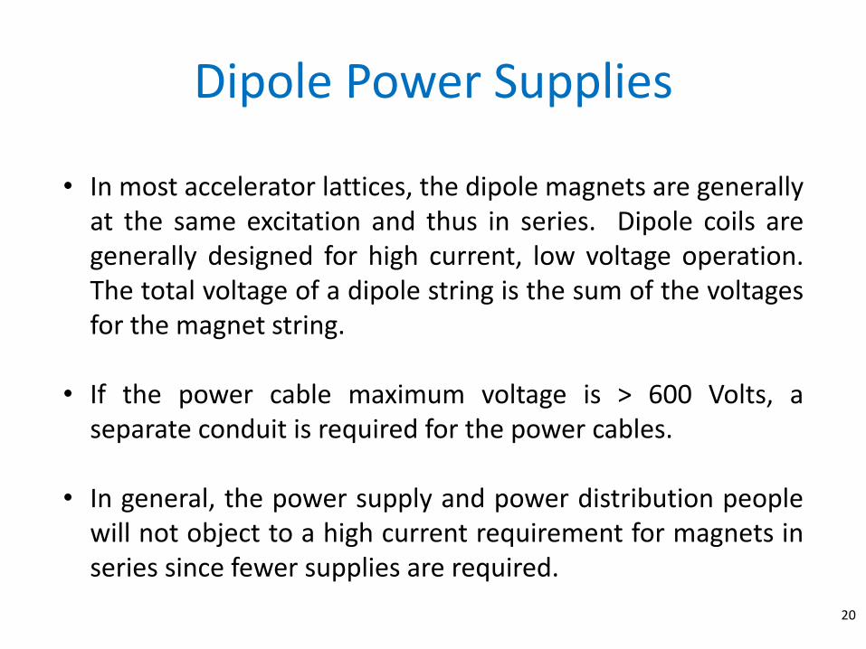
• In most accelerator lattices, the dipole magnets are generally at the same excitation and thus in series. Dipole coils are generally designed for high current, low voltage operation. The total voltage of a dipole string is the sum of the voltages for the magnet string.

• If the power cable maximum voltage is > 600 Volts, a separate conduit is required for the power cables.

• In general, the power supply and power distribution people

will not object to a high current requirement for magnets in series since fewer supplies are required.

Quadrupole Power Supplies

21

• Quadrupole magnets are usually individually powered or connected in short series strings (families).

• Since there are so many quadrupole circuits, quadrupole coils are generally designed to operate at lower current and higher voltage.

Sextupole Power Supplies

22

• Sextupole are generally operated in a limited number of series strings (families). Their effect is distributed around the lattice. In many lattices, there are a maximum of two series strings.

• Since the excitation requirements for sextupole magnets is

generally modest, sextupole coils can be designed to operate at either high or low currents.

Power Consumption

23

• The raw cost of power varies widely depending on location and constraints under which power is purchased.

• In the Northwest US, power is cheap. • Power is often purchased at low prices by

negotiating conditions where power can be interrupted.

• The integrated cost of power requires consideration of the lifetime of the facility.

• The cost of cooling must also be factored into the cost of power.

Coil Cooling

24

• In this section, we shall temporarily abandon the MKS system of units and use the mixed engineering and English system of units.

• Assumptions – The water flow requirements are based on the heat capacity of the

water and assumes no temperature difference between the bulk water and conductor cooling passage surface.

– The temperature of the cooling passage and the bulk conductor temperature are the same. This is a good assumption since we usually specify good thermal conduction for the electrical conductor.

Pressure Drop

25

2sec

ft 32.2=onaccelerati nalgravitatio=

sec

ftcity water velo=

) as same (unitsdiameter holecircuit water =

) as same (unitslength circuit water =

units) (nofactor friction =

psi drop pressure

where

g

v

Ld

dL

f

ΔP

2

433.02

g

v

d

LfP

1 ft/s = 0.3048 m/s

9.8 m/s2

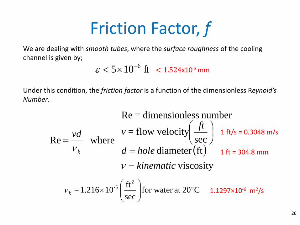
Friction Factor, f

26

ft 105 6

We are dealing with smooth tubes, where the surface roughness of the cooling channel is given by;

Under this condition, the friction factor is a function of the dimensionless Reynold’s Number.

viscosity

ftdiameter sec

velocityflow=

number essdimensionl=Re

whereRe

kinematic

holed

ftvvd

k

C20at for water sec

ft 101.216=

25-

k

< 1.524x10-3 mm

1 ft/s = 0.3048 m/s

1 ft = 304.8 mm

1.1297×10-6 m2/s

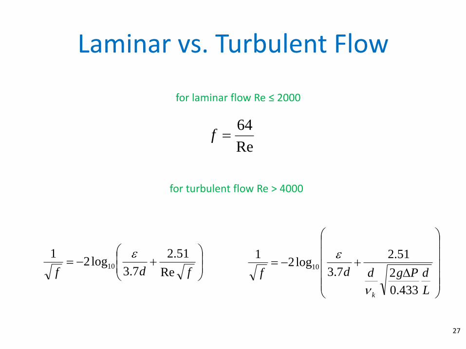
Re

64f

Re

51.2

7.3log2

110

fdf

Laminar vs. Turbulent Flow

27

for laminar flow Re ≤ 2000

for turbulent flow Re > 4000

L

dPgddf

k 433.0

2

51.2

7.3log2

110

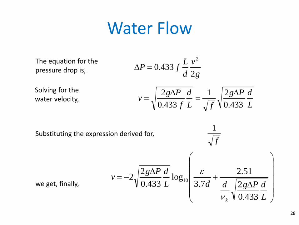
Water Flow

28

2

433.02

g

v

d

LfP

L

dPg

fL

d

f

Pgv

433.0

21

433.0

2

The equation for the pressure drop is,

Solving for the water velocity,

f

1Substituting the expression derived for,

L

dPgddL

dPgv

k 433.0

2

51.2

7.3log

433.0

22 10

we get, finally,

Coil Temperature Rise

29

gpmq

kWPCT

8.3

Based on the heat capacity of water, the water temperature rise for a flow through a thermal load is given by,

Assuming good heat transfer between the water stream and the coil conductor, the maximum conductor temperature (at the water outlet end of the coil) is the same value.

1 gpm = 0.0630901 liter/s 1 gpm = 3.78541 liter/s

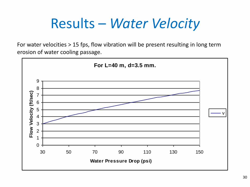
For L=40 m, d=3.5 mm.

0

1

2

3

4

5

6

7

8

9

30 50 70 90 110 130 150

Water Pressure Drop (psi)

Flo

w V

elo

cit

y (

ft/s

ec)

v

For water velocities > 15 fps, flow vibration will be present resulting in long term erosion of water cooling passage.

Results – Water Velocity

30

Results – Reynolds Number

31

For L=40 m, d=3.5 mm.

0

1000

2000

3000

4000

5000

6000

7000

8000

30 50 70 90 110 130 150

Pressure Drop (psi)

Reyn

old

s N

um

ber

Re

Results valid only for Re > 4000 (turbulent flow).

Results – Water Temperature Rise

32

Desirable temperature rise for Light Source Synchrotrons < 10oC. Maximum allowable temperature rise (assuming 20oC. input water) < 30oC for long potted coil life.

For P=0.62 kW, L=40 m, d=3.5 mm.

0

2

4

6

8

10

12

14

16

18

30 50 70 90 110 130 150

Pressure Drop

Tem

pera

ture

Ris

e (

deg

.C)

DT

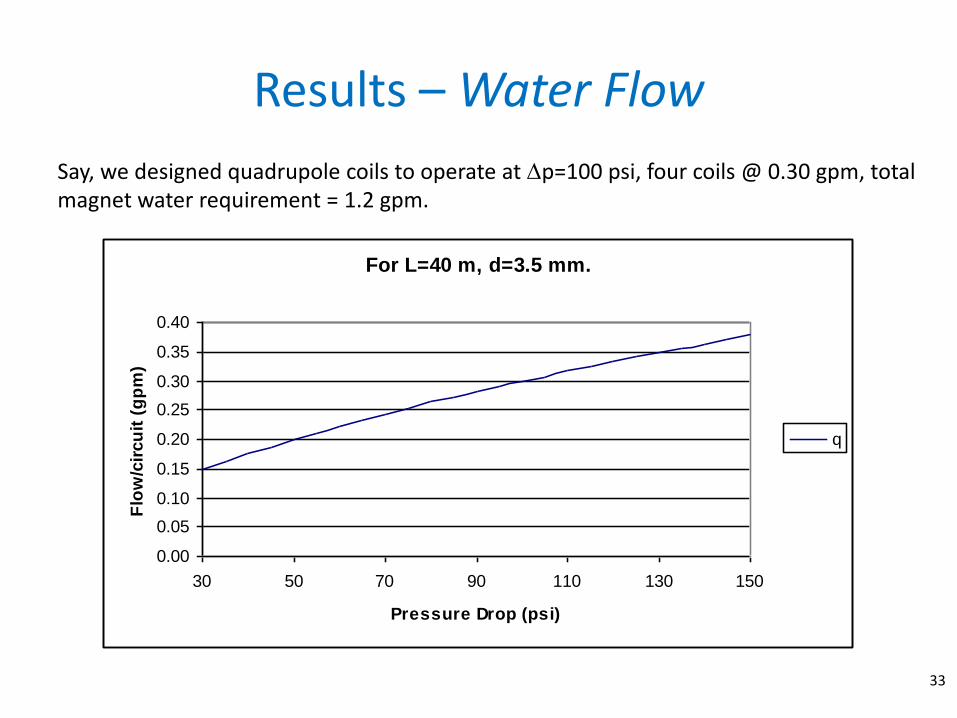
Results – Water Flow

33

For L=40 m, d=3.5 mm.

0.00

0.05

0.10

0.15

0.20

0.25

0.30

0.35

0.40

30 50 70 90 110 130 150

Pressure Drop (psi)

Flo

w/c

ircu

it (

gp

m)

q

Say, we designed quadrupole coils to operate at p=100 psi, four coils @ 0.30 gpm, total magnet water requirement = 1.2 gpm.

Sensitivities

34

• Coil design is an iterative process.

• If you find that you selected coil geometries parameters which result in calculated values which exceed the design limits, then you have to start the design again. – P is too large for the maximum available pressure drop in

the facility.

– Temperature rise exceeds desirable value.

• The sensitivities to particular selection of parameters must be evaluated.

Sensitivities – Number of Water Circuits

35

22

2433.0 Lv

g

v

d

LfP

The required pressure drop is given by,

where L is the water circuit length.

w

ave

N

KNL=

K = 2, 4 or 6 for dipoles, quadrupoles or sextupoles, respectively. N = Number of turns per pole. NW = Number of water circuits.

wN

Qv

2

2

ww

ave

N

Q

N

KNLvP

Substituting into the pressure drop expression,

3

1

wNP

Pressure drop can be decreased by a factor of eight if the number of water circuits are doubled.

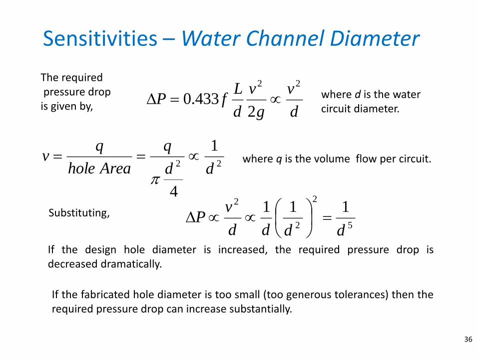
Sensitivities – Water Channel Diameter

d

v

g

v

d

LfP

22

2433.0

The required pressure drop is given by,

where d is the water circuit diameter.

22

1

4

dd

q

Areahole

qv

where q is the volume flow per circuit.

5

2

2

2 111

dddd

vP

Substituting,

If the design hole diameter is increased, the required pressure drop is decreased dramatically.

If the fabricated hole diameter is too small (too generous tolerances) then the required pressure drop can increase substantially.

36

Summary

37

• Excitation current for several kinds of magnets were derived.

• Saturation must be avoided (η≥0.98).

• Current densities canonical numbers where presented.

• Magnet power and its implications with the facility was discussed.

• Coil cooling parameters was shown.

• Coil design is an iterative process.

Next…

38

• Stored Energy

• Magnetic Forces

• Dynamic effects (eddy currents)