lecture 30: linear variation theory the material in this lecture covers the following in atkins

Lecture 30: Linear Variation Theory The material in this lecture covers the following in Atkins.

14.7 Heteronuclear diatomic molecules (c) The variation principle

Lecture on-line Linear Variation Theory (PowerPoint) Linear Variation Theory (PDF)

Handout for this lecture

The Linear Variation Method

We have a Hamiltonian H with the eigenfunctions ψna nd eigenvalues En give n by t he SWE

Hψn = Enψn

Let u s l ook a t th e groundstat e ψ1 with t he energ y E1 .

W e would lik e to fi nd a wavefuncti on Φ1 fo r which the

energy

W = ∫ Φ

1

∗H Φ

1d τ / ∫ Φ

1

∗Φ

1d τ

i s clos e to E1

The linear variation method

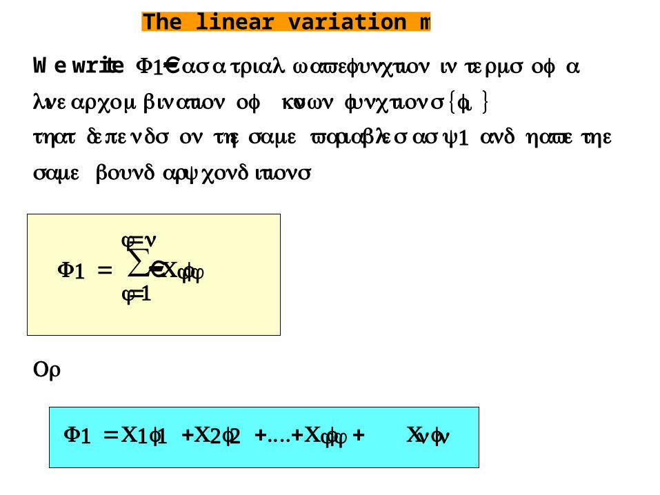
We write Φ1 as a ttriri aall wavefuncti on in te rms of a

line ar combinati on of kno wn function s {fi }

tha t depen ds on th e same variable s a s ψ1 a nd hav e the

sa meboundary conditions

Φ1 = ∑j=1

j=n Cjfj

Or

Φ1 = C1f1 +C2f2 +....+Cjfj + Cnfn


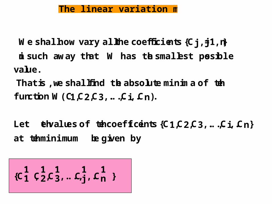
We shall now vary all the coefficients {Cj ,j=1,n}

in such a way that W has the smallest possible

value.

That is ,we shall find the absolute minima of the

function W(C1,C2,C3,.....,Ci,..Cn).

Let the values of the coefficients {C1,C2,C3,.....,Ci,..Cn}

at the minimum be given by

{C11 ,C

12,C

13, ...,C

1j ,..C

1n }


What do we know about this particular coefficients ?

We know that if we look at the derivatives of W

δ W

δ Ci

= W’(C1,C2,..... ,Cn)

The n ’W (C11 ,C

12,C

13, ...,C

1j ,..C

1n ) = 0

W e shall us e thi s fac t to fi nd { C11 ,C

12,C

13, ...,C

1j ,..C

1n}


First let us substitute the expression for Φ1 i nto the

expressi on fo r W. The denomenato r of I1 is

⌡⎮⌠

Φ1 ∗ Φ1 dτ = ⌡⎮⌠

⎝⎜⎜⎜⎛

⎠⎟⎟⎟⎞

∑j=1

j=n Cj*fj*

⎝⎜⎜⎜⎛

⎠⎟⎟⎟⎞

∑k=1

k=n Ckfk

W e shal l assume tha t a ll functi ons {fj j=1,n} ar e rea l and

tha t al l coefficient s {Cj=1,n} are real


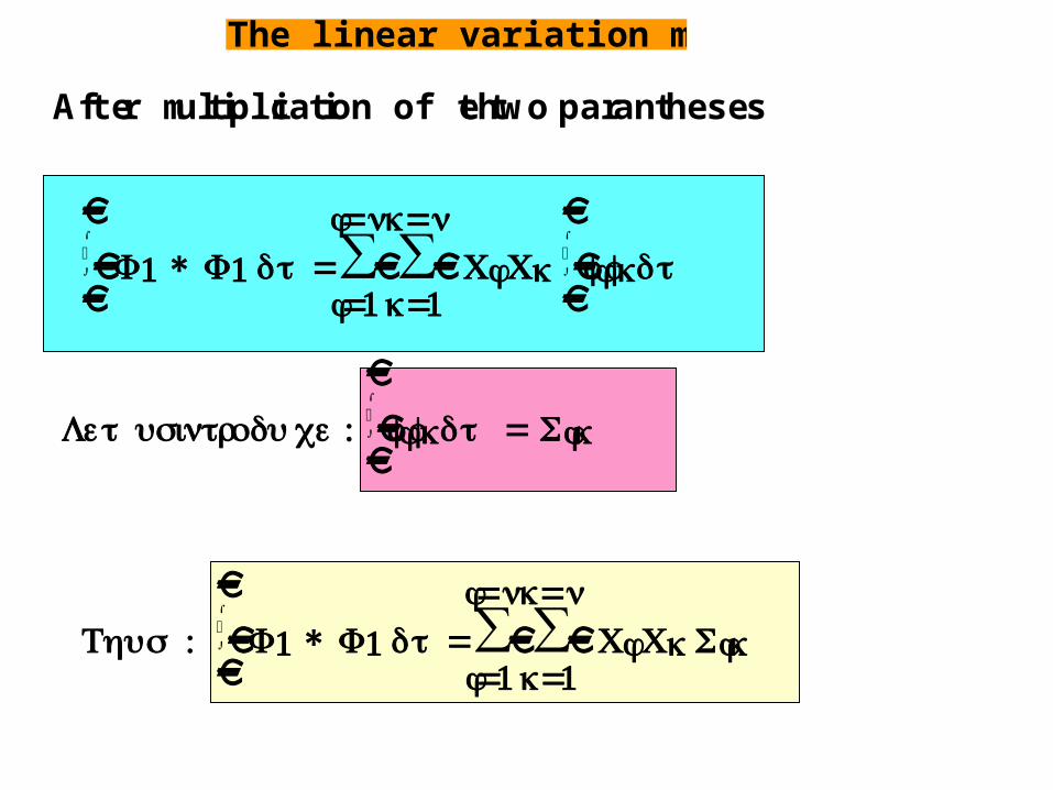
After multiplication of the two parantheses

⌡⎮⌠

Φ1 ∗ Φ1 dτ =∑j=1

j=n ∑k=1

k=n Cj Ck ⌡

⎮⌠

fjfkdτ

Le t usintroduce : ⌡⎮⌠

fjfkdτ = Sjk

Thu s : ⌡⎮⌠

Φ1 ∗ Φ1 dτ =∑j=1

j=n ∑k=1

k=n Cj Ck Sjk


For the numerator in the expression for I1 we have

⌡⎮⌠

Φ1∗ H Φ1dτ = ⌡⎮⌠

⎝⎜⎜⎜⎛

⎠⎟⎟⎟⎞

∑j=1

j=n Cj*fj* H

⎝⎜⎜⎜⎛

⎠⎟⎟⎟⎞

∑k=1

k=n Ckfk

O r aft er multiplicati on ofparanthesis

⌡⎮⌠

Φ1∗ H Φ1dτ = =∑j=1

j=n ∑k=1

k=n Cj Ck ⌡

⎮⌠

fj H fkdτ


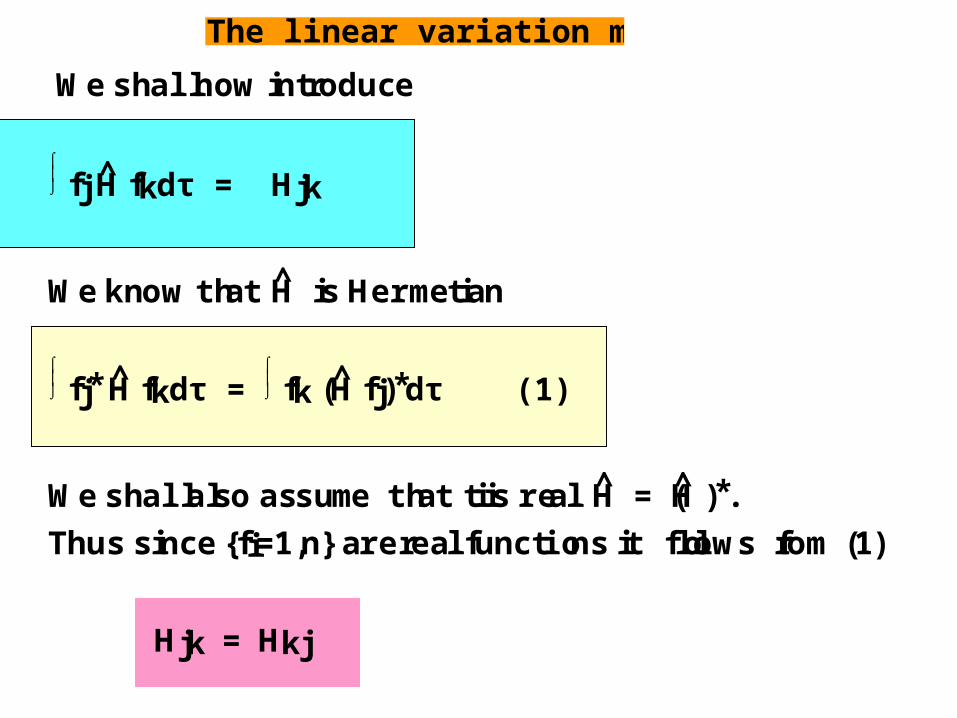
We shall now introduce

⌡⎮⌠

fj H fkdτ = Hjk

We know that H is Hermetian

⌡⎮⌠

fj* H fkdτ = ⌡⎮⌠

fk (H fj)*dτ (1)

We shall also assume that it is real H = (H )*.

Thus since {fi=1,n} are real functions it follows from (1)

Hjk = Hkj


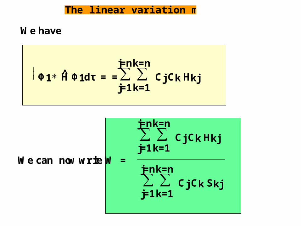
We have

⌡⎮⌠

Φ1∗ H Φ1dτ = =∑j=1

j=n ∑k=1

k=n Cj Ck Hkj

We can now write W =

∑j=1

j=n ∑k=1

k=n Cj Ck Hkj

∑j=1

j=n ∑k=1

k=n Cj Ck Skj


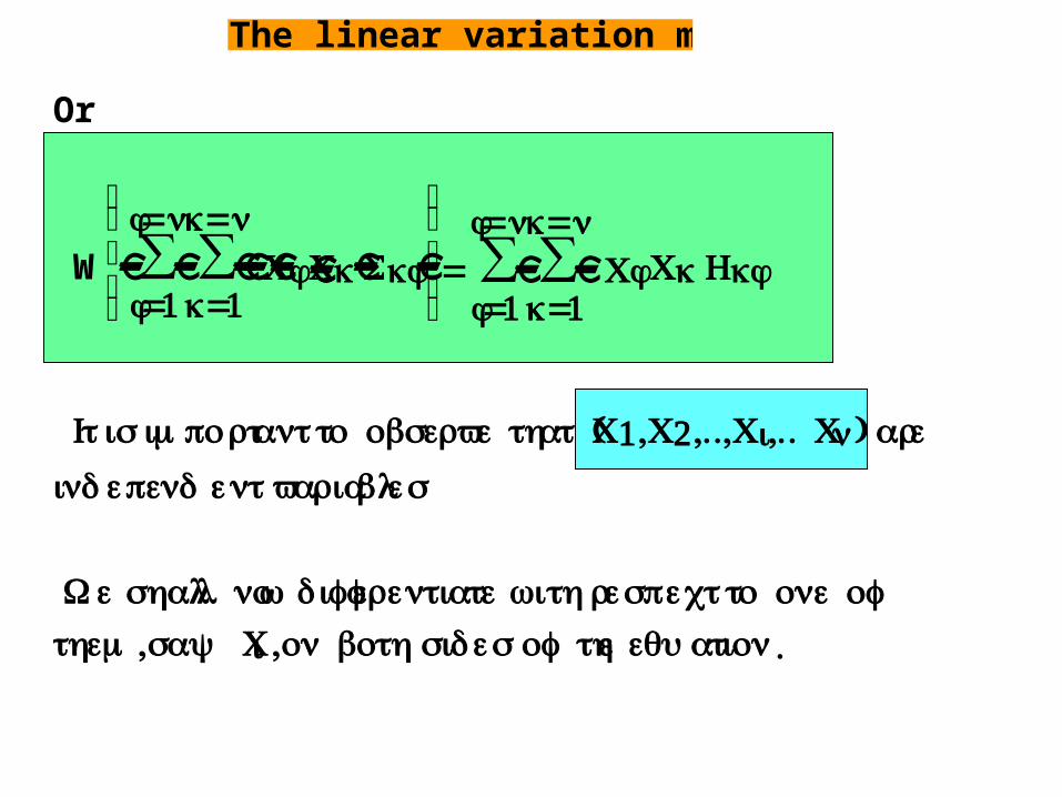
Or

W⎝⎜⎜⎜⎛

⎠⎟⎟⎟⎞

∑j=1

j=n ∑k=1

k=n C j Ck Skj = ∑

j=1

j=n ∑k=1

k=n C j Ck Hkj

It is important t o observ e tha (t C1,C2,..,Ci,.. Cn) are

independe nt variables

W e shal l no w differentiat e wi th respect t o one of

them,say C i , on bothside s of th e equation.


We have

δ W

δ Ci ⎝⎜⎜⎜⎛

⎠⎟⎟⎟⎞

∑j=1

j=n ∑k=1

k=n C j Ck Skj + W

δδCi

⎝⎜⎜⎜⎛

⎠⎟⎟⎟⎞

∑j=1

j=n ∑k=1

k=n C j Ck Skj =

δ

δ Ci j = 1

j = n

∑

k = 1

k = n

∑ Cj

Ck

Hkj

⎛

⎝

⎜

⎜

⎞

⎠

⎟

⎟

Let u s no w loo k a t δ

δCi⎝⎜⎜⎜⎛

⎠⎟⎟⎟⎞

∑j=1

j=n ∑k=1

k=n C j Ck Skj =


Since we differentiate a sum by differentiating

each term from rules for differentiating a product

⎝⎜⎜⎜⎛

⎠⎟⎟⎟⎞

∑j=1

j=n ∑k=1

k=n

δδCi( C j Ck Skj ) =

⎝⎜⎜⎜⎛

⎠⎟⎟⎟⎞

∑j=1

j=n ∑k=1

k=n [

δC jδCiCk Skj +

δCk δCi Cj Skj]

Since (C1,C2,..,Ci,.. Cn) ar e independe nt variables

δCjδCi = 0 i f ≠i j

δCjδCi = 1 i f i= j ;

δCjδCi = δij


⎝⎜⎜⎜⎛

⎠⎟⎟⎟⎞

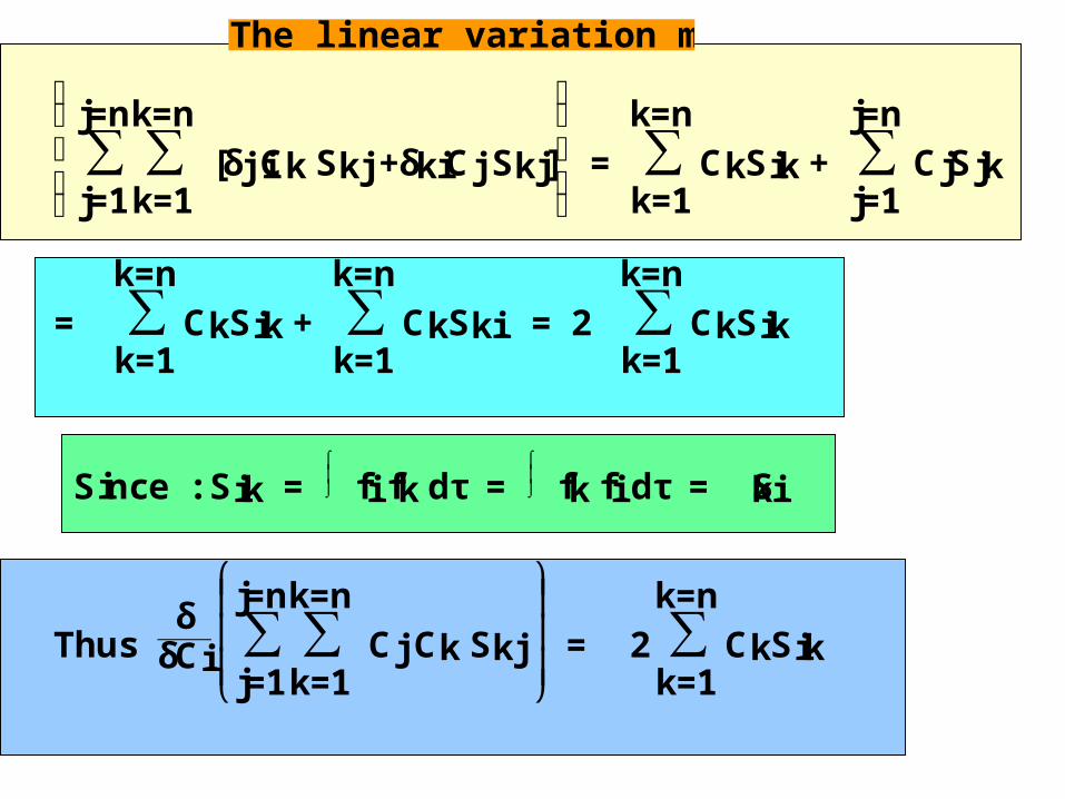
∑j=1

j=n ∑k=1

k=n [δjiCk Skj +δkiCj Skj] = ∑

k=1

k=n CkSik + ∑

j=1

j=n CjSjk

= ∑k=1

k=n CkSik + ∑

k=1

k=n CkSki = 2 ∑

k=1

k=n CkSik

Since : Sik = ⌡⎮⌠

fi fk dτ = ⌡⎮⌠

fk fi dτ = Ski

Thus δ

δCi⎝⎜⎜⎜⎛

⎠⎟⎟⎟⎞

∑j=1

j=n ∑k=1

k=n Cj Ck Skj = 2 ∑

k=1

k=n CkSik


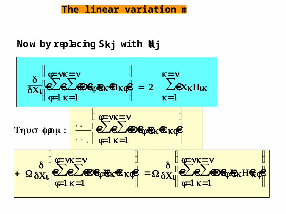
Now by replacing Skj with Hkj

δδCi

⎝⎜⎜⎜⎛

⎠⎟⎟⎟⎞

∑j=1

j=n ∑k=1

k=n C j Ck Hkj = 2 ∑

k=1

k=n CkHik

Thu s from: δ W

δ Ci ⎝⎜⎜⎜⎛

⎠⎟⎟⎟⎞

∑j=1

j=n ∑k=1

k=n C j Ck Skj

+ WδδCi

⎝⎜⎜⎜⎛

⎠⎟⎟⎟⎞

∑j=1

j=n ∑k=1

k=n C j Ck Skj = W

δδCi

⎝⎜⎜⎜⎛

⎠⎟⎟⎟⎞

∑j=1

j=n ∑k=1

k=n C j CkH kj


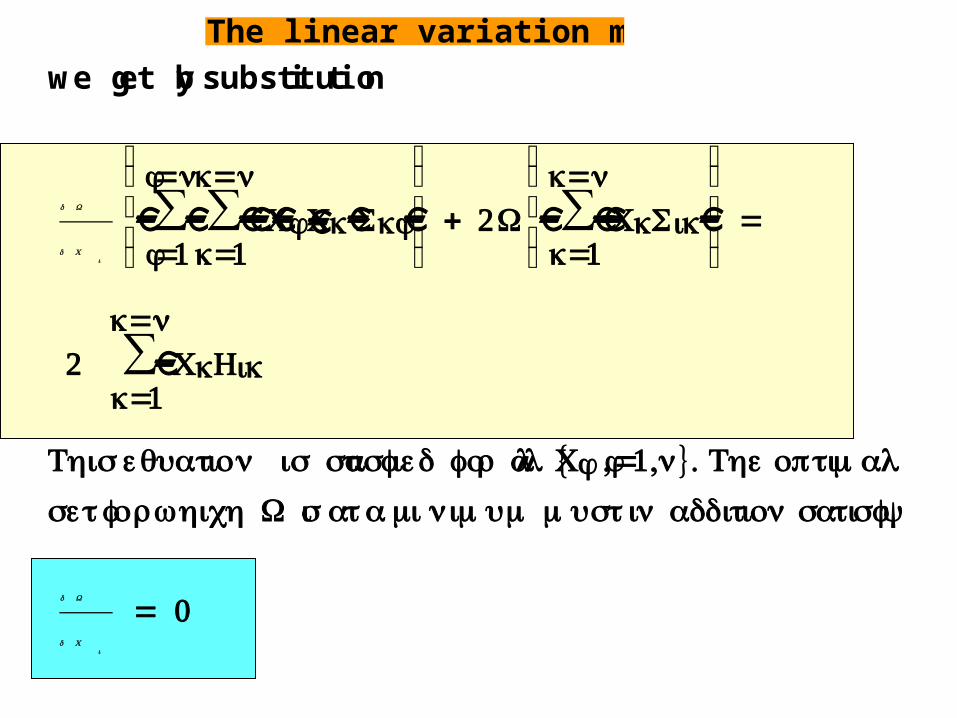
we get by substitution

δ W

δ Ci

⎝⎜⎜⎜⎛

⎠⎟⎟⎟⎞

∑j=1

j=n ∑k=1

k=n C j Ck Skj + 2 W

⎝⎜⎜⎜⎛

⎠⎟⎟⎟⎞

∑k=1

k=n CkSik =

2 ∑k=1

k=n CkHik

This equation is satisfie d fo r al {l Cj ,j=1,n}. The optimal

set for whic h W i s a t aminimu mmus t i n additi on satisfy

δ W

δ Ci

= 0


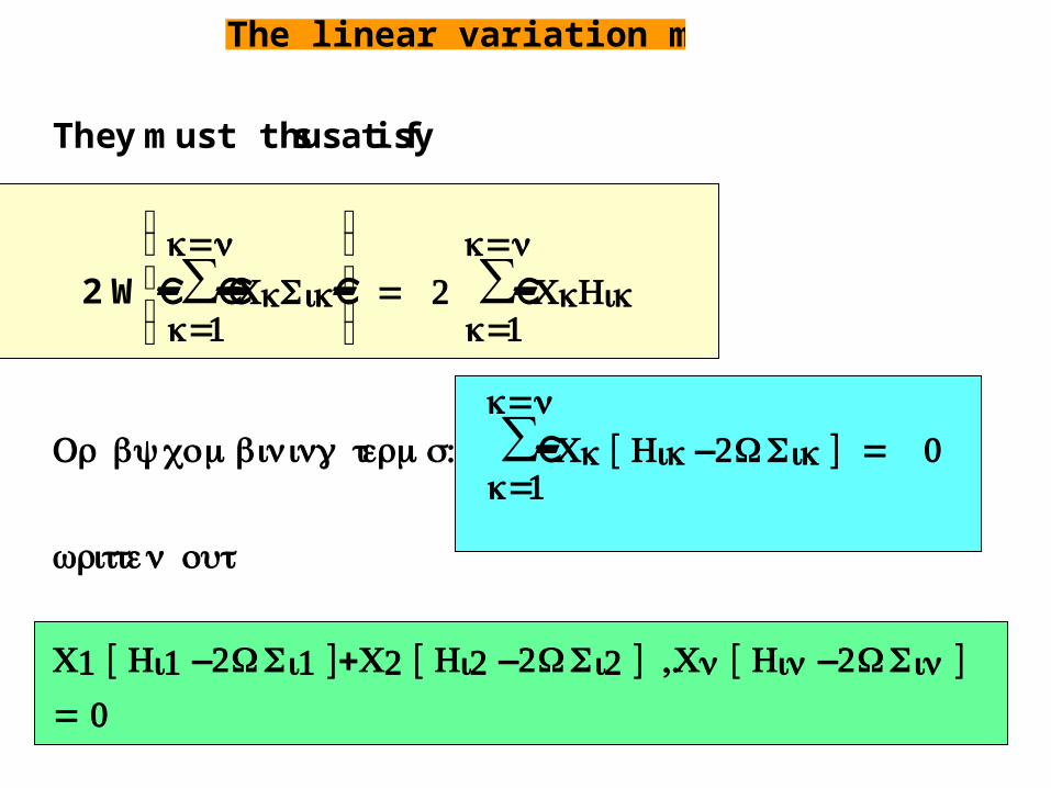
They must thus satisfy

2 W⎝⎜⎜⎜⎛

⎠⎟⎟⎟⎞

∑k=1

k=n CkSik = 2 ∑

k=1

k=n CkHik

Or b y combini ng terms: ∑k=1

k=n Ck [ Hik –2WSi k ] = 0

writte n out

C1 [ Hi1 –2WSi1 ]+C2 [ Hi2 –2WSi2 ] ,.Cn [ Hin –2WSi n ]

= 0


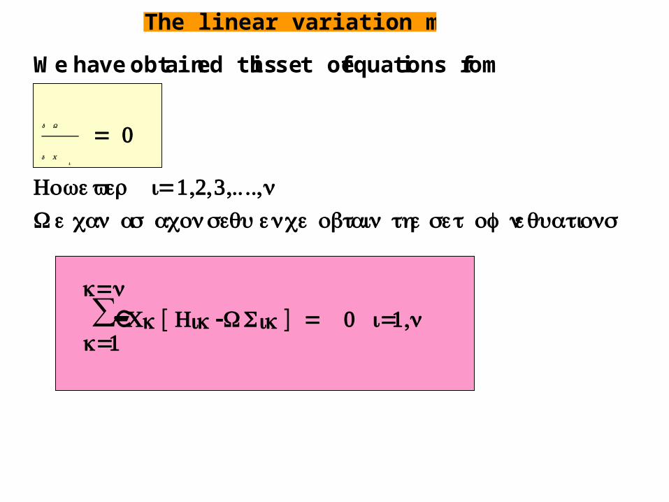
We have obtained this set of equations from

δ W

δ Ci

= 0

Howev er i= 1,2,3,.. ..,nW e ca n a s a consequenc e obtai n th e se t of nequations

∑k=1

k=n Ck [ Hik -WSi k ] = 0 =i 1,n


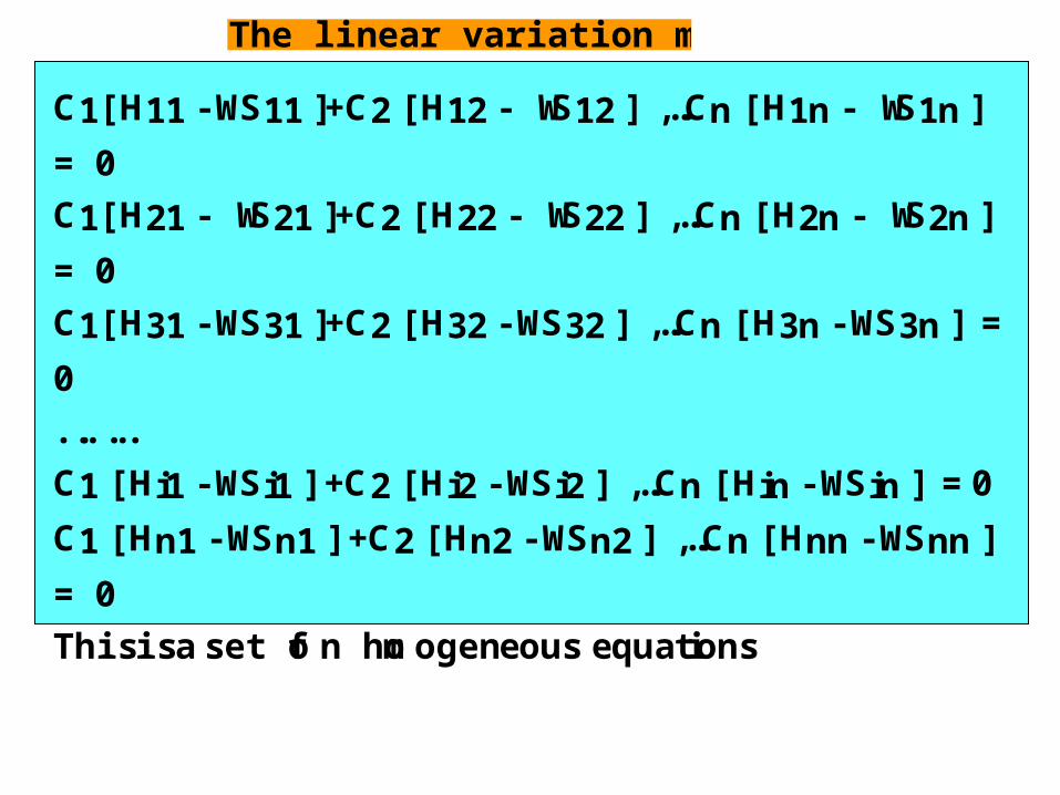
C1[ H11 -WS11 ]+C2 [ H12 - WS12 ] ,...Cn [ H1n - WS1n ]

= 0

C1[ H21 - WS21 ]+C2 [ H22 - WS22 ] ,...Cn [ H2n - WS2n ]

= 0

C1[ H31 -WS31 ]+C2 [ H32 -WS32 ] ,...Cn [ H3n -WS3n ] =

0

.......

C1 [ Hi1 -WSi1 ] +C2 [ Hi2 -WSi2 ] ,...Cn [ Hin -WSin ] = 0

C1 [ Hn1 -WSn1 ] +C2 [ Hn2 -WSn2 ] ,...Cn [ Hnn -WSnn ]

= 0

This is a set of n homogeneous equations


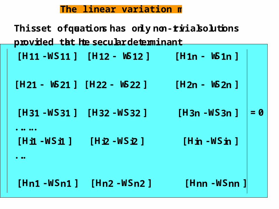
This set of equations has only non-trivial solutions

provided that the secular determinant

[ H11 -WS11 ] [ H12 - WS12 ] [ H1n - WS1n ]

[ H21 - WS21 ] [ H22 - WS22 ] [ H2n - WS2n ]

[ H31 -WS31 ] [ H32 -WS32 ] [ H3n -WS3n ] = 0

.......

[ Hi1 -WSi1 ] [ Hi2 -WSi2 ] [ Hin -WSin ]

....

[ Hn1 -WSn1 ] [ Hn2 -WSn2 ] [ Hnn -WSnn ]


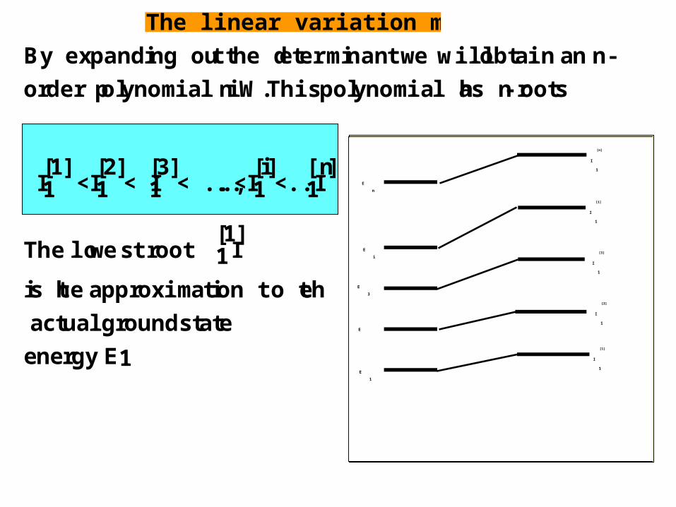
By expanding out the determinant we will obtain an n-

order polynomial in W.This polynomial has n-roots

I[1]1 <I

[2]1 < I

[3]1 < .....,<I

[i]1 <..I

[n]1

The lowest root I[1]1

is the approximation to the

actual groundstate

energy E1E

1

E

E

3

E

i

E

n

I

1

[1]

I

1

[2]

I

1

[3]

I

1

[i]

I

1

[n]


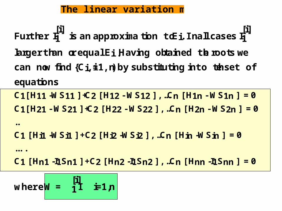
Further I[i]1 is an approximation to Ei. In all cases I

[i]1

larger than or equal Ei. Having obtained the roots we

can now find {Ci,i=1,n) by substituting into the set of

equationsC1[ H11 -WS11 ]+C2 [ H12 - WS12 ] ,...Cn [ H1n - WS1n ] = 0

C1[ H21 - WS21 ]+C2 [ H22 - WS22 ] ,...Cn [ H2n - WS2n ] = 0

..

C1 [ Hi1 -WSi1 ] +C2 [ Hi2 -WSi2 ] ,...Cn [ Hin -WSin ] = 0

....

C1 [ Hn1 -I1Sn1 ] +C2 [ Hn2 -I1Sn2 ] ,...Cn [ Hnn -I1Snn ] = 0

where W = I[i]1 i=1,n


What you should learn from this lecture1. You should understand that in linear variationtheory the trial wavefunction is written as a linear combination of KNOWN functionswhere the relative contribution from each functionis optimized.

2. You should know how the set of linear equationsare generated and why the secular determinant must bezero and how this is used to determine theenergies.

3. You should be able to derive the equation in the case where n=2

lecture 30: linear variation theory the material in this lecture covers the following in atkins

Documents