Lecture 3: W-algebras

1 / 40

1. Overwiew on W-algebras

Recall: The four fundamental physical theoriesand the corresponding algebraic structures.

PV A− CFT

Zhu

quantization,,QFT − V A

cl.limitoo

Zhu

PA− CM

affiniz.

FF

quantization

22 QM −AAcl.limitoo

affiniz.

WW

Note: The classical limit corresponds to taking the associated gradedof a filtered AA or VA.

The Zhu algebra [Zhu96] is an AA (resp. PA) associated to a positive

energy VA (resp. PVA).2 / 40

W-algebras provide a rich family of examples, parametrized byg: simple Lie algebra, and f ∈ g: nilpotent, appearing in all 4fundamental aspects:

Wclz (g, f)

Zhu

quantization++Wk(g, f)

cl.limitoo

Zhu

Wcl,fin(g, f)

affiniz.

GG

quantization

22Wfin(g, f)

cl.limitoo

affiniz.

WW

They were introduced separately and played important roles in

different areas of math. Only later it became fully clear the relations

between them.

3 / 40

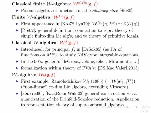
Classical finite W-algebra: Wcl,fin(g, f)

I Poisson algebra of functions on the Slodowy slice [Slo80].

Finite W-algebra: Wfin(g, f)

I First appearance in [Kos78,Lyn79]: Wfin(g, fpr) ' Z(U(g))

I [Pre02]: general definition; connection to repr. theory ofsimple finite-dim Lie alg’s, and to theory of primitive ideals.

Classical W-algebra: Wclz (g, f)

I Introduced, for principal f , in [DrSok85] (as PA offunctions on M∞), to study KdV-type integrable equations.

I In the 90’s: gener.’s [deGroot,Delduc,Feher, Miramontes... ]

I formalization within theory of PVA’s: [DS,Kac,Valeri,2013]

W-algebra: Wk(g, f)

I First example: Zamolodchikov W3 (1985) (=W(sl3, fpr)).

(“non-linear” ∞-dim Lie algebra, extending Virasoro).

I [Fei.Fre.90], [Kac,Roan,Wak.03] general construction via aquantization of the Drinfeld-Sokolov reduction. Applicationto representation theory of superconformal algebras.

4 / 40

The links among the four appearances of W-algebras are morerecent:

I [Gan,Gin,2002]: finite W-algebra as a quantization of the

Slodowy slice: Wfin(g, f)cl.limit−→ Wcl,fin(g, f).

I [DS,Kac,2006], (indep. [Ara07]): the (H-twisted) Zhualgebra of the W-algebra Wk(g, f) is isomorphic to thefinite W-algebra Wfin(g, f). (Hence, their categories ofirreducible representations are equivalent.)

5 / 40

2. The Poisson structure on the Slodowy slice.

Set up:

I g: simple Lie algebra.

I (· | ·): non-degenerate symmetric invariant form.

I Identify Φ : g∼→ g∗ , a 7→ (a, ·)

I f ∈ g: a nilpotent element. By the Jacobson-MorozovTheorem, we can include it in an sl2-triple (f, h = 2x, e).

The corresponding Slodowy slice is the affine space:

S = Φ(f + ge) ⊂ g∗

Claim: S ⊂ g∗ is a Poisson submanifold.

Exercise 1: If ξ ∈ S, the sympl. form ωξ on the sympl. leaveAd∗G(ξ) restricts to a sympl. form on TξS ∩ Tξ Ad∗G(ξ)Exercise 2: S intersects transversally the symplectic leafs:TξS ∩ Tξ Ad∗G(ξ) = Tξg

∗ (i.e. ad∗(g)(ξ) ∩ Φ(ge) = g∗).The Claim follows by these two exercises

6 / 40

In order to quantize the theory, we shall describe the Slodowyslice S as a Hamiltonian reduction of the Poisson manifold g∗

(with the Kirillov-Kostant Poisson bracket).

Recall: the general procedure of Hamiltonian reduction:

Ham.red.(M,χ,N) = µ−1(χ)/N

where N is a Lie group with a Hamiltonian action on M andmomentum map µ : M → n∗, and χ ∈ n∗ is ad∗N -invariant.

Set up:

I adx-eignespace decomposition: g =⊕

i∈ 12Z gi

I On g 12

we have the non-degenerate skewsymmetric form

ω(u, v) = (f |[u, v])

and we let ` ⊂ g 12

be a maximal isotropic subspace.

Exercise 3: Check that ω is a non-degenerate skewsymmetricform on g 1

2.

7 / 40

I Consider the nilpotent subalgebra n = `⊕ g≥1 ⊂ g (and thecorresponding unipotent Lie group N).

I Consider the coadjoint action of N on g∗.

Exercise 4: Prove that the coadjoint action of N on thePoisson manifold g∗ is a Hamiltonian action, with momentummap µ : g∗ → n∗ given by restriction.Exercise 5: The dual of the momentum map µ∗ : n→ g is theinclusion map.

I Let χ = (f | ·)|n ∈ n∗.

I Its preimage via the momentum map is µ−1(χ) = Φ(f +n⊥)

Exercise 6: Check that χ([n, n]) = 0. Use this to prove that χis ad∗N -invariant.

I Hence, we have the corresponding Hamiltonian reduction:

Ham.Red.(g∗, N, χ) = µ−1(χ)/N = Φ(f + n⊥)/N

8 / 40

Proposition [Gan, Ginzburg, 2001]: The adjoint action

N × (f + ge)∼−→ f + n⊥

is an isomorphism of affine varieties.

Exercise 7: Prove it.

Conclusion: It follows that

Ham.Red.(g∗, N, χ) = Φ(f + n⊥)/N ' Φ(f + ge) = S

(It is not hard to check that the Poisson structure is the same.)

9 / 40

By passing to the corresponding algebras of (polynomial)functions, we get the Hamiltonian reduction definition of theclassical finite W-algebra:

W cl,fin(g, f) = C[S]

=(C[g∗]/C[g∗]f vanish. on µ−1(χ)

)adµ∗(n)

=(S(g)

/S(g)n− (f |n)n∈n

)ad n= N/I

where N =x ∈ S(g)

∣∣ n, x ⊂ I and I = S(g)n− (f |n)n∈n

10 / 40

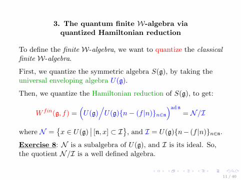
3. The quantum finite W-algebra viaquantized Hamiltonian reduction

To define the finite W-algebra, we want to quantize the classicalfinite W-algebra.

First, we quantize the symmetric algebra S(g), by taking theuniversal enveloping algebra U(g).

Then, we quantize the Hamiltonian reduction of S(g), to get:

W fin(g, f) =(U(g)

/U(g)n− (f |n)n∈n

)ad n= N/I

where N =x ∈ U(g)

∣∣ [n, x] ⊂ I

, and I = U(g)n− (f |n)n∈n.

Exercise 8: N is a subalgebra of U(g), and I is its ideal. So,the quotient N/I is a well defined algebra.

11 / 40

We want to see that, indeed, W fin(g, f) is a quantization ofW cl,fin(g, f).

We define the following Kazhdan filtration of the universalenveloping algebra U(g): for a ∈ gi, we let ∆(a) = 1− i (we callthis the “conformal weight” of a). Then, we let

FnU(g) = Spana1 . . . as

∣∣∣∆(a1) + · · ·+ ∆(as) ≤ n

Exercise 9: We have: ∆([a, b]) = ∆(a) + ∆(b)− 1. Hence, wehave a filtration of the algebra U(g), and the associated gradedis the Poisson algebra S(g).

Note: n− (f |n) is “homogeneous” w.r.t. conf. weight. TheKazhdan filtration of U(g) induces a filtr on Wfin(g, f), and:

Proposition [Gan Ginzburg 01]: grWfin.(g, f) ' Wcl.fin.(g, f).

Exercise 10: prove it.

12 / 40

4. The quantum affine W-algebra

The quantum affine W-algebra Wk(g, f) is a vertex algebra.

It is not known how to define it via quantized Hamiltonianreduction. There is a cohomological definition, via the so calledBRST cohomology.

It was first defined by [Feigin and Frenkel.1990] for evennilpotent f , and generalized by [Kac, Roan and Wakimoto,2003].

To every vertex algebra (conformal, positive energy) V , there isassociated an associative algebra called its Zhu algebra Zhu(V ),which describes its representations. In the sense that there is anequivalence of categories

positive energy repr’s of V↔

fin.dim. repr’s of Zhu(V )

We proved in [D.S., Kac 2006] that ZhuWk(g, f) ' Wfin.(g, f).13 / 40

5. The classical affine W-algebra via“affine” Hamiltonian reduction

Set up. It is the same as before:g: a semisimple Lie algebra. (e, h, f) ∈ g: an sl2-triple in g.g =

⊕i∈ 1

2Z gi: decomposition in eigenspaces of 1

2(adh).

Construction: (Affine Hamiltonian reduction)

I We start with the Affine PVA: V(g) = S(F[∂]g), with

[aλb] = [a, b] + (a|b)λ , a, b ∈ g ,

I Consider the differential algebra ideal 〈a− (f |a)〉a∈g≥1.

The quotient V(g)/〈a− (f |a)〉a∈g≥1is NOT a PVA.

I If we take invariants w.r.t. λ-action of the Lie conformalalgebra C[∂]g≥ 1

2, we get a PVA.

14 / 40

Definition: The classical affine W-algebra is

W(g, f) =(V(g)

/〈a− (f |a)〉a∈g≥1

)adλ(F[∂]g≥ 12

)= N/I

whereN =

x ∈ V(g)

∣∣ g≥ 12 λx ⊂ I[λ]

and

I = 〈a− (f |a)〉a∈g≥1(diff. alg. ideal)

Exercise 11: Check that N is a Poisson vertex subalgebra ofV(g) and I is its idea. Hence, W(g, f) is a Poisson vertexalgebra.

Structure Thm: as a differential algebra, W(g, f) isisomorphic to the algebra of differential polynoamials in finitelymany variables wi, i = 1, . . . ,dim(gf ) (Premet’s generators):

W (g, f) ' F[w(n)i |

i = 1,. . ., dim(gf )n ∈ Z+

]

Note: the same is true for all other types of W -algebras.15 / 40

Natural questions:

Problem 1: Find explicit formulas for generators widim(gf )i=1 .

Problem 2: Find explicit formulas for the λ-brackets amonggenerators: wiλwj ∈ F[λ]W (g, f).

Problem 3: Construct an integrable hierarchy of Hamilt. eq’sfor the PVA structure of W(g, f).

Example / Exercise 12: W (sl2, f) ' V(Vir); correspondingintegrable hierarchy: KdV.

GOAL:

For a classical Lie algebra g = glN , slN , soN , spN and arbitrarynilpotent f ∈ g we have a new method, based on the notions ofAdler type operators and generalized quasideterminants, whichgives a complete answer to all three problems at the same time,for every nilpotent element f .

16 / 40

6. Lax equations

Definition [P. Lax 1968] Let L = L(t), P = P (t) be linearoperators, depending on t. The corresponding Lax equation is

(1)dL

dt= [P,L]

Usually, L = ∂n + ... (pseudodiff. operator) and P = (Lk/n)+.

Then: [Lax “theorem”] Equation (1) is integrable, and∫Res∂ L

k/n, k ≥ 1, are integrals of motion in involution.

Example: Lax main example:

L = ∂2 + u, P = ∂3 + 2u∂ + u′.

Then [P,L] = u′′′ + uu′, hence

dL

dt= [P,L]⇔ KdV :

du

dt= u′′′ + uu′.

17 / 40

Main Issue (which hasn’t been completely resolved to date):the Lax Equation (1) should be selfconsistent.

Example: consider the operators L = ∂3 + u, P = (Lk/3)+.

Then the Lax equation (1) for k = 1 is: dudt1

= u′ , butfor k = 2 it is

du

dt= 2u′∂ + u′′

which is inconsistent.

18 / 40

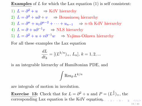
Examples of L for which the Lax equation (1) is self consistent:

1) L = ∂2 + u ⇒ KdV hierarchy

2) L = ∂3 + u∂ + v ⇒ Boussinesq hierarchy

3) L = ∂n + u1∂n−2 + · · ·+ un−1 ⇒ n-th KdV hierarchy

4) L = ∂ + u∂−1v ⇒ NLS hierarchy

5) L = ∂2 + u+ v∂−1w ⇒ Yajima-Oikawa hierarchy

For all these examples the Lax equation

dL

dtk= [(Lk/n)+, Ln], k = 1, 2, ...

is an integrable hierarchy of Hamiltonian PDE, and∫Res∂ L

k/n

are integrals of motion in involution.

Exercise 13: Check that for L = ∂2 + u and P = (L32 )+, the

corresponding Lax equation is the KdV equation.19 / 40

Main Goal: for each nilpotent f ∈ g, we construct a Laxoperator L(∂), such that:

(2)dL

dtk=

[(Lk/p1

)+, L

](k ∈ Z)

is an integrable hierarchy of compatible evolution equations,with the infinitely many integrals of motion in involution:∫

Res∂ Tr Lk/p1 (k ∈ Z)

Moreover:

1) L(∂) contains all generators of the W -algebra W (glN , f);

2) we have an Adler identity for the λ-brackets;

3) all Lax eq.s (2) are Hamiltonian w.r.t. the PVA W (glN , f)

(This solves all our 3 problems at the same time!)

20 / 40

7. First ingredient: Adler type operators

Definition. Let V be a PVA with λ-bracket · λ ·.A(∂) ∈ MatN×N V((∂−1)) is of Adler type (w.r.t. · λ ·) if:

Aij(z)λAhj(w) = Ahj(w+λ+∂)(z−w−λ−∂)−1(Aik)∗(λ−z)

−Ahj(z)(z−w−λ−∂)−1Aik(w) .

Example. V = V(glN ) (with aλb = [a, b] + (a|b)λ). Then:

E + ∂1 =

e11 + ∂ e21 . . . eN1

e12 e22 + ∂ . . . eN2...

. . ....

e1N . . . eNN + ∂

∈ MatN×NV(glN )

is of Adler type. (Notation: eij = standard basis of glN .)

Exercise 14: Check this.21 / 40

Adler type operators are very useful to construct Integrable Systems!

Theorem.[D.S., Kac, Valeri,’15] Let: V a PVA; A(∂) an

operator of Adler type; K ≥ 1 s.t. A(∂)1K exists. Let∫

hn =∫

Res∂Tr(A(∂)nK ) ∈ V/∂V , n ∈ Z+

They are pairwise in involution:

∫hm,

∫hn = 0 ∀m,n

Hence, integrable hierarchy of Hamiltonian eq’s:

du

dtn= ∫hn, u

This hierarchy is equivalently written in Lax form:

dA(∂)

dtn= [(A(∂)

nK)

+, A(∂)] , n ∈ Z+

22 / 40

Idea: To construct integrable systems of Hamiltonianequations, we want Adler operators.

Question: How do we construct new Adler operators?(So far, only one example: E + ∂1 ∈ MatN×N (glN ).)

Answer: we use (generalized) quasideterminant

23 / 40

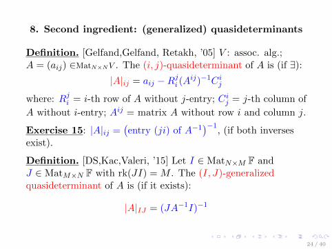
8. Second ingredient: (generalized) quasideterminants

Definition. [Gelfand,Gelfand, Retakh, ’05] V : assoc. alg.;A = (aij) ∈MatN×NV . The (i, j)-quasideterminant of A is (if ∃):

|A|ij = aij −Rji (Aij)−1Cij

where: Rji = i-th row of A without j-entry; Cij = j-th column of

A without i-entry; Aij = matrix A without row i and column j.

Exercise 15: |A|ij =(entry (ji) of A−1

)−1, (if both inverses

exist).

Definition. [DS,Kac,Valeri, ’15] Let I ∈ MatN×M F andJ ∈ MatM×N F with rk(JI) = M . The (I, J)-generalizedquasideterminant of A is (if it exists):

|A|IJ = (JA−1I)−1

24 / 40

Theorem/Observation. If A(∂) is of Adler type for V, thenany its generalized quasideterminant |A(∂)|I,J is again of Adlertype.

Exercise 16: prove it.

25 / 40

9) Construction of the Lax operator for W(g, f)

Step 1:Let ψ : g→ End V be a finite-dimensional representation of gs.t. (a|b) = trV ψ(a)ψ(b) is non-degenerate.Choose a basis uii∈B of g and let uii∈B be the dual basis.

The associated ancestor Lax operator is

LV (∂) = ∂1V +∑i∈B

uiψ(ui) ∈ V(g)[∂]⊗ EndV

(It is independent of the choice of basis).

26 / 40

Step 2:The descendant Lax operator LV,f (∂) for the PVA W (g, f) isconstructed as follows:

Let J : V → V [∆] be the projection and I : V [∆] → V theinclusion (∆ = max eigenvalue for ϕ(x)).Let ρ : V(g)→ V (g) be the differential algebra homomorphismdefined by:

ρ(a) = π≤ 12(a) + (f |a), a ∈ g.

Then LV,f (∂) is the generalized quasi-determinant:

LV,f (∂) = (J(ρ(LV (∂))−1I))−1

27 / 40

First Main Theorem∀ g, V, f , the descendant Lax operator LV,f (∂) is an r1 × r1

matrix pseudo-differential operator with leading term ∂p1 andcoefficients in W (g, f):

LV,f (∂) = ∂p11r1×r1 + . . . ∈ W (g, f)((∂−1))⊗ EndV [∆]

(Note: LV,f (∂) encodes all generators of W (g, f).)

28 / 40

Second Main TheoremLet g = glN , ψ be its standard representation in V = FN ,f ∈ g nilpotent, associated to the partition N = p1 + · · ·+ ps,(p1 ≥ · · · ≥ ps) and let r1 be the multiplicity of p1.Then LV,f (∂) satisfies the following Adler identity (based on thefamous Adler’s map, 1979)

L(z)λL(w) =(1⊗ L(w+λ+∂)

)iz(z−w−λ−∂)−1

(L∗(λ−z)⊗ 1

)Ω

− Ω(L(z)⊗ iz(z−w−λ−∂)−1L(w)

)where iz stands for the geometric series expansion for large z,and Ω is the permutation of factors.

Classical Lie algebras: A similar theorem holds for allclassical Lie alg.s: slN , soN , spN , with V = FN . [DSKV, 2018]

(Note: The Adler identity encodes all λ-brackets in W (g, f).)

29 / 40

As we said, Adler type operators are automatically Laxoperators, i.e. they produce an integrable hierarchy ofHamiltonian eq.s in Lax form [DSKV, 2015-18]. As a corollary:

Third Main Theorem

1)∫hn =

∫Res∂ TrLV,f (∂)

np1 ∈W (g, f)/∂W are Hamiltonian

functionals in involution:

∫hm,

∫hn = 0 for all m,n

2) We thus get an integrable hierarchy of Hamiltonianequations for W (g, f)

du

dtn= ∫ hn, u

3) This hierarchy can be written in Lax form:

dLV,f (∂)

dtn= [LV,f (∂)

np1+ , LV,f (∂)]

30 / 40

Historical Remark

I Drinfeld and Sokolov [1985] constructed an integrableHamiltonian hierarchy of PDE for any simple Lie algebra gand its principal nilpotent element f , using Kostant’s cyclicelements.

I In [DSKV, 2015] we extended their method for any simpleLie algebra g and its nilpotent elements f of “semisimpletype”.(There are very few such elements in classical g, but about12 of nilpotents in exceptional g are such: 13 out of 20 inE6, 21 out of 44 in E7, 27 out of 69 in E8, 11 out of 15 inF4, 3 out of 4 in G2 [Elashvili-Kac-Vinberg, 2013]).

I The Lax operator method generalizes, in case of classical g,the DS hierarchy to arbitrary nilpotent f ∈ g.

31 / 40

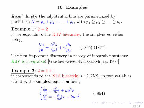
10. Examples

Recall: In glN the nilpotent orbits are parametrized bypartitions N = p1 + p2 + · · ·+ ps, with p1 ≥ p2 ≥ · · · ≥ ps.Example 1: 2 = 2it corresponds to the KdV hierarchy, the simplest equationbeing:

∂u

∂t=∂3u

∂x3+ u

∂u

∂x(1895) (1877)

The first important discovery in theory of integrable systems:KdV is integrable! [Gardner-Green-Kruskal-Miura, 1967]

Example 2: 2 = 1 + 1it corresponds to the NLS hierarchy (=AKNS) in two variablesu and v, the simplest equation being

∂u∂t = ∂2u

∂x2+ ku2v

∂v∂t = − ∂2v

∂x2v − kuv2

(1964)

32 / 40

Example 3: 3 = 3: corresponds to the Boussinesq hierarchy,the simplest equation being the Boussinesq equations

∂u∂t = ∂v

∂x∂v∂t = ∂3u

∂x3+ u∂u∂x

(1872)

Example 4: 3 = 1 + 1 + 1: corresponds to the 3 wave equation.

Example 5: 3 = 2 + 1: corresponds to the Yajima-Oikawahiearchy in three variables u, v, w, the simplest equationdescribing sonic-Langmuir solitons:

∂u∂t = −∂2u

∂x2+ uw

∂v∂t = ∂2v

∂x2− vw

∂w∂t = ∂

∂x(uv)

(1976)

33 / 40

Example 6: N = N :it corresponds to the N -th Gelfand-Dickey hierarchy (1975)

Example 7: N = 2 + 1 + · · ·+ 1:it corresponds to the N−2-component Yajima-Oikawa hierarchy

Example 8: N = p+ p+ · · ·+ p (r times): corresponds to thep-th r × r-matrix Gelfand-Dickey hierarchy

Exercise 16: check (some of) these examples.

34 / 40

11. Multiplicative Poisson vertex algebrasand Hamiltonian difference equations

Parallel Theories:

I PVA ⇒ Hamiltonian PDE

I Multiplicative PVA ⇒ Hamilt. differential-difference eq.s

The theory of mPVA & Hamiltonian differential-differenceequations is much less developed then the theory of PVA &Hamiltonian PDE’s.

There are so far only very partial classification results and somewell studied examples of integrable Hamiltonian eq’s.

35 / 40

DefinitionA multiplicative Poisson vertex algebra (mPVA) is an algebra Vwith an automorphism D, and a λ-bracket fλg ∈ V[λ, λ−1] s.t.

(sesquilinearity) D(f)λg = λ−1fλg , fλD(g) = λDfλg(skewsymmetry) fλg = −←gλ−1D−1f,(Jacobi identity) fλgµh − gµfλh = fλgλµh.

(Leibniz rule) fλgh = fλgh+ gfλh.

36 / 40

Remark: mPVA ⇔ “local” Poisson algebra (V, S) (= a PA Vwith an automorphism S, s.t. Sna, b = 0 for |n| >> 0.)

Proof: aλb =∑

n∈Z λnSna, b is a mPVA structure on V.

Exercise 17: prove it.

Example: The most famous example of a “local” PA is theFaddeev-Takhtajan-Volkov algebra [1986]: V = F[un|n ∈ Z],with D(un) = un+1, and Poisson bracket

um, un =umun ((δm+1,n − δm,n+1) (1− um − un)

−um+1δm+2,n + un+1δm,n+2) .

The corresponding mPVA λ-bracket:

uλu = u(1 + λD)u(1 + λD)u− u(1 + λ−1D−1)u(1 + λ−1D−1)u

− u(λD − λ−1D−1)u

Exercise 18: Check this formula.

37 / 40

Basic Lemma. Let V be a mPVA. Let · , · = · λ ·|λ=1.

I V := V/(D − 1)V (= local functionals) is a Lie algebra withLie bracket · λ ·|λ=1;

I LA representation of V on V (= functions).

DefinitionThe Hamiltonian equation associated to the mPVA V and theHamiltonian functional ∫ h ∈ V is

du

dt= ∫ h, u , u ∈ V

Integrability: ∃∫h0=

∫h,∫h1,∫h2. . . (lin.ind.) integrals of

motion in involution: ∫hm,

∫hn = 0 ∀m,n

38 / 40

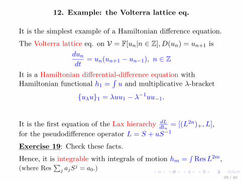
12. Example: the Volterra lattice eq.

It is the simplest example of a Hamiltonian difference equation.

The Volterra lattice eq. on V = F[un|n ∈ Z], D(un) = un+1 is

dundt

= un(un+1 − un−1), n ∈ Z

It is a Hamiltonian differential-difference equation withHamiltonian functional h1 =

∫u and multiplicative λ-bracket

uλu1 = λuu1 − λ−1uu−1.

It is the first equation of the Lax hierarchy dLdtn

= [(L2n)+, L],

for the pseudodifference operator L = S + uS−1

Exercise 19: Check these facts.

Hence, it is integrable with integrals of motion hm = ∫ ResL2m,(where Res

∑j ajS

j = a0.)

39 / 40

The well-known various versions of: the Toda lattice hierarchies,the Bogoyavlensky lattice hierarchies, the discrete KPhierarchies, and many other integrable Hamiltoniandifferential-difference equations can be treated along the samelines.

The general theory is work in progress.

40 / 40