lecture 3: svm dual, kernels and multiple classes

Lecture 3: SVM dual, kernels and regression

C19 Machine Learning Hilary 2015 A. Zisserman

• Primal and dual forms

• Linear separability revisted

• Feature maps

• Kernels for SVMs

• Regression• Ridge regression• Basis functions

SVM – review• We have seen that for an SVM learning a linear classifier

f(x) = w>x+ b

is formulated as solving an optimization problem over w :

minw∈Rd

||w||2 + CNXi

max (0,1− yif(xi))

• This quadratic optimization problem is known as the primal problem.

• Instead, the SVM can be formulated to learn a linear classifier

f(x) =NXi

αiyi(xi>x) + b

by solving an optimization problem over αi.

• This is know as the dual problem, and we will look at the advantages

of this formulation.

Sketch derivation of dual formThe Representer Theorem states that the solution w can always be

written as a linear combination of the training data:

w =NXj=1

αjyjxj

Proof: see example sheet .

Now, substitute for w in f(x) = w>x+ b

f(x) =

⎛⎝ NXj=1

αjyjxj

⎞⎠>x+ b =NXj=1

αjyj³xj>x

´+ b

and for w in the cost function minw ||w||2 subject to yi³w>xi+ b

´≥ 1,∀i

||w||2 =⎧⎨⎩Xj

αjyjxj

⎫⎬⎭>⎧⎨⎩Xk

αkykxk

⎫⎬⎭ =Xjk

αjαkyjyk(xj>xk)

Hence, an equivalent optimization problem is over αj

minαj

Xjk

αjαkyjyk(xj>xk) subject to yi

⎛⎝ NXj=1

αjyj(xj>xi) + b

⎞⎠ ≥ 1,∀iand a few more steps are required to complete the derivation.

Primal and dual formulationsN is number of training points, and d is dimension of feature vector x.

Primal problem: for w ∈ Rd

minw∈Rd

||w||2 + CNXi


Dual problem: for α ∈ RN (stated without proof):

maxαi≥0

Xi

αi−1

2

Xjk

αjαkyjyk(xj>xk) subject to 0 ≤ αi ≤ C for ∀i, and

Xi

αiyi = 0

• Need to learn d parameters for primal, and N for dual

• If N << d then more efficient to solve for α than w

• Dual form only involves (xj>xk). We will return to why this is an

advantage when we look at kernels.

Primal and dual formulations

Primal version of classifier:

f(x) = w>x+ b

Dual version of classifier:

f(x) =NXi

αiyi(xi>x) + b

At first sight the dual form appears to have the disad-

vantage of a K-NN classifier — it requires the training

data points xi. However, many of the αi’s are zero. The

ones that are non-zero define the support vectors xi.

Support Vector Machine

w

Support VectorSupport Vector

b

||w||

wTx + b = 0

support vectors

f(x) =Xi

αiyi(xi>x) + b

C = 10 soft margin

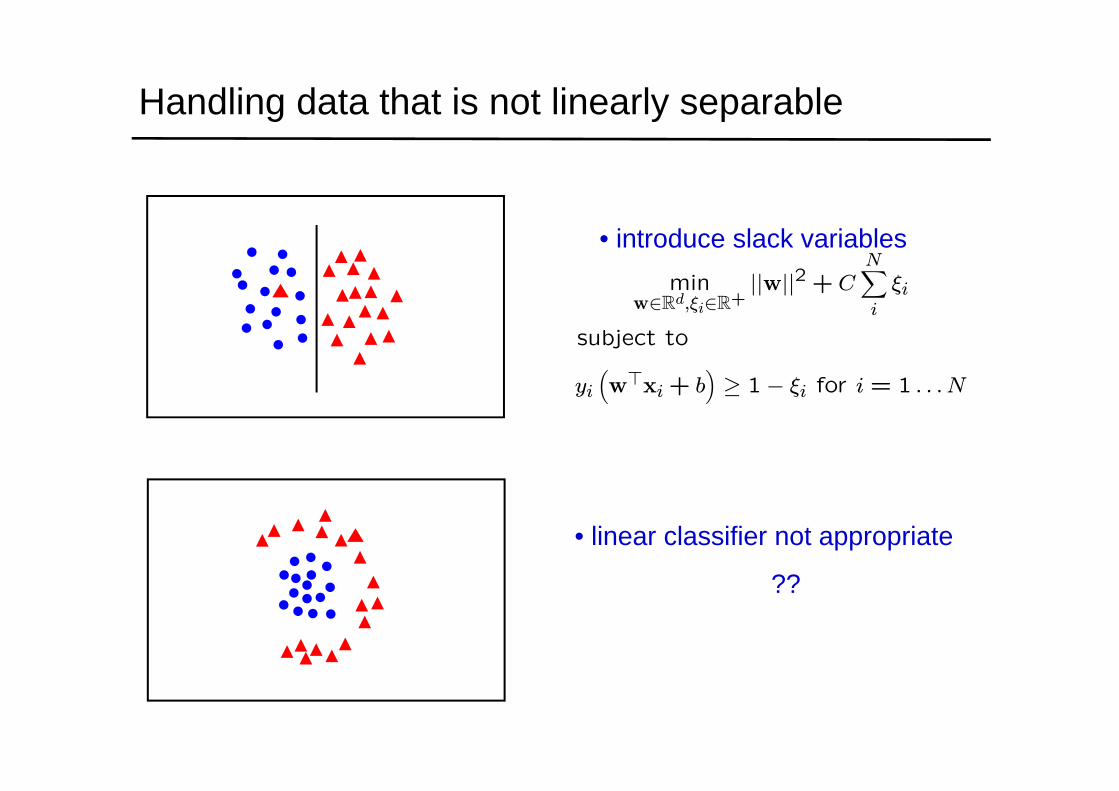
Handling data that is not linearly separable

• introduce slack variables

• linear classifier not appropriate

??

minw∈Rd,ξi∈R+

||w||2 + CNXi

ξi

subject to

yi³w>xi+ b

´≥ 1− ξi for i = 1 . . . N

Solution 1: use polar coordinates

0

0

• Data is linearly separable in polar coordinates

• Acts non-linearly in original space

r

θ

θ

r

Φ :

Ãx1x2

!→

Ãrθ

!R2 → R2

> 0< 0

Solution 2: map data to higher dimension

0

0

• Data is linearly separable in 3D

• This means that the problem can still be solved by a linear classifier

Φ :

Ãx1x2

!→

⎛⎜⎝ x21x22√2x1x2

⎞⎟⎠ R2→ R3

SVM classifiers in a transformed feature space

f(x) = 0

Rd RD

Φ

Φ : x→ Φ(x) Rd → RD

Learn classifier linear in w for RD:

f(x) = w>Φ(x) + b

Φ(x) is a feature map

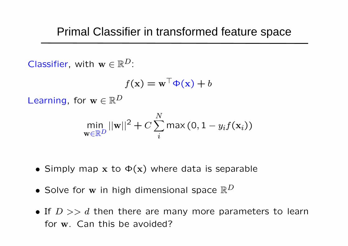
Classifier, with w ∈ RD:

f(x) = w>Φ(x) + b

Learning, for w ∈ RD

minw∈RD

||w||2 + CNXi


• Simply map x to Φ(x) where data is separable

• Solve for w in high dimensional space RD

• If D >> d then there are many more parameters to learn

for w. Can this be avoided?

Primal Classifier in transformed feature space

Classifier:

f(x) =NXi

αiyi xi>x+ b

→ f(x) =NXi

αiyiΦ(xi)>Φ(x) + b

Learning:

maxαi≥0

Xi

αi −1

2

Xjk

αjαkyjykxj>xk

→ maxαi≥0

Xi

αi −1

2

Xjk

αjαkyjykΦ(xj)>Φ(xk)

subject to

0 ≤ αi ≤ C for ∀i, andXi

αiyi = 0

Dual Classifier in transformed feature space

• Note, that Φ(x) only occurs in pairs Φ(xj)>Φ(xi)

• Once the scalar products are computed, only the N dimensional

vector α needs to be learnt; it is not necessary to learn in the

D dimensional space, as it is for the primal

• Write k(xj,xi) = Φ(xj)>Φ(xi). This is known as a Kernel

Classifier:

f(x) =NXi

αiyi k(xi,x) + b

Learning:

maxαi≥0

Xi

αi −1

2

Xjk

αjαkyjyk k(xj,xk)

subject to

0 ≤ αi ≤ C for ∀i, andXi

αiyi = 0

Dual Classifier in transformed feature space

Special transformations

Φ :

Ãx1x2

!→

⎛⎜⎝ x21x22√2x1x2

⎞⎟⎠ R2→ R3

Φ(x)>Φ(z) =³x21, x

22,√2x1x2

´⎛⎜⎝ z21z22√2z1z2

⎞⎟⎠= x21z

21 + x22z

22 + 2x1x2z1z2

= (x1z1 + x2z2)2

= (x>z)2

Kernel Trick• Classifier can be learnt and applied without explicitly computing Φ(x)

• All that is required is the kernel k(x, z) = (x>z)2

• Complexity of learning depends on N (typically it is O(N3)) not on D

Example kernels

• Linear kernels k(x,x0) = x>x0

• Polynomial kernels k(x,x0) =³1+ x>x0

´dfor any d > 0

— Contains all polynomials terms up to degree d

• Gaussian kernels k(x,x0) = exp³−||x− x0||2/2σ2

´for σ > 0

— Infinite dimensional feature space

f(x) =NXi

αiyik(xi,x) + b

N = size of training data

weight (may be zero)

support vector

SVM classifier with Gaussian kernel

Gaussian kernel k(x,x0) = exp³−||x− x0||2/2σ2

´Radial Basis Function (RBF) SVM

f(x) =NXi

αiyi exp³−||x− xi||2/2σ2

´+ b

-0.8 -0.6 -0.4 -0.2 0 0.2 0.4 0.6 0.8 1-0.6

-0.4

-0.2

0

0.2

0.4

0.6

feature x

feat

ure

y

RBF Kernel SVM Example

• data is not linearly separable in original feature space

σ = 1.0 C =∞f(x) = 1

f(x) = 0

f(x) = −1

f(x) =NXi


´+ b

σ = 1.0 C = 100

Decrease C, gives wider (soft) margin

σ = 1.0 C = 10

f(x) =NXi


´+ b

σ = 1.0 C =∞

f(x) =NXi


´+ b

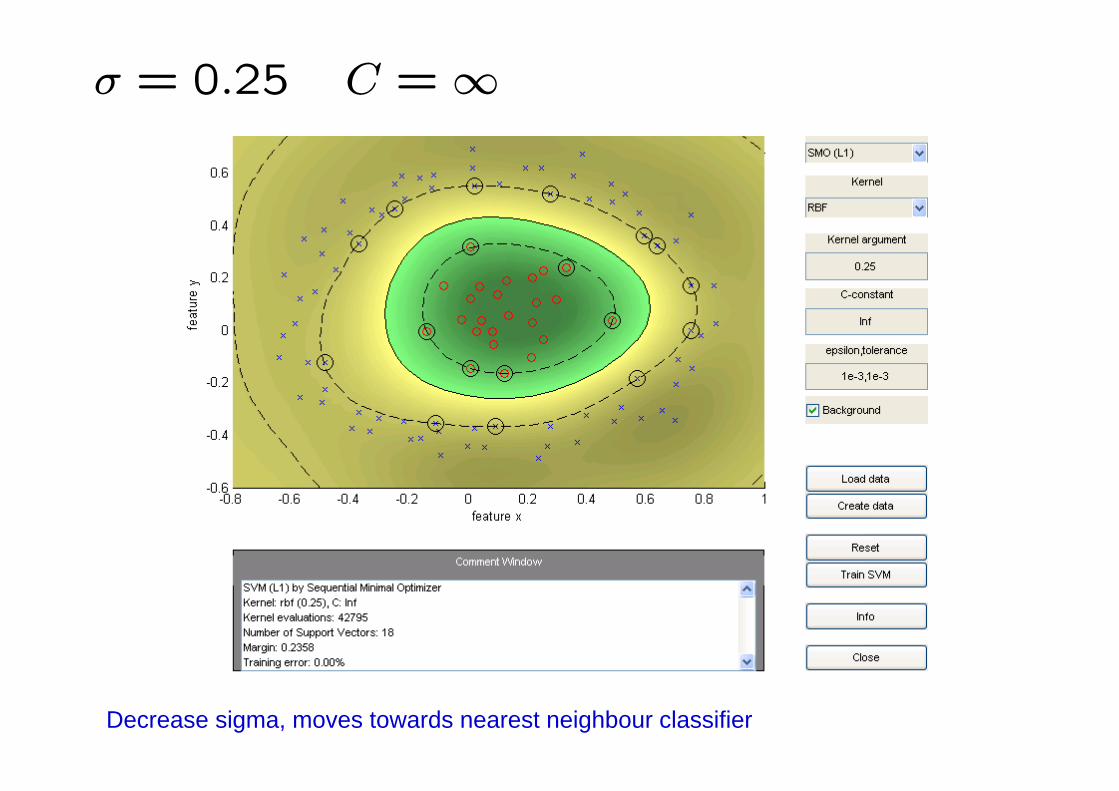
σ = 0.25 C =∞

Decrease sigma, moves towards nearest neighbour classifier

σ = 0.1 C =∞

f(x) =NXi


´+ b

Kernel Trick - Summary• Classifiers can be learnt for high dimensional features spaces, without actually having to map the points into the high dimensional space

• Data may be linearly separable in the high dimensional space, but not linearly separable in the original feature space

• Kernels can be used for an SVM because of the scalar product in the dual form, but can also be used elsewhere – they are not tied to the SVM formalism

• Kernels apply also to objects that are not vectors, e.g.

k(h, h0) =Pkmin(hk, h

0k) for histograms with bins hk, h

0k

y

Regression

• Suppose we are given a training set of N observations

((x1, y1), . . . , (xN, yN)) with xi ∈ Rd, yi ∈ R

• The regression problem is to estimate f(x) from this data

such that

yi = f(xi)

Learning by optimization

• As in the case of classification, learning a regressor can be formulated as an optimization:

loss function regularization

• There is a choice of both loss functions and regularization

• e.g. squared loss, SVM “hinge-like” loss

• squared regularizer, lasso regularizer

Minimize with respect to f ∈ FNXi=1

l (f(xi), yi) + λR (f)

Choice of regression function – non-linear basis functions

• Function for regression y(x,w) is a non-linear function of x, butlinear in w:

f(x,w) = w0 + w1φ1(x) + w2φ2(x) + . . .+ wMφM (x) = w>Φ(x)

• For example, for x ∈ R, polynomial regression with φj(x) = xj :

f(x,w) = w0 + w1φ1(x) + w2φ2(x) + . . .+ wMφM (x) =MXj=0

wjxj

e.g. for M = 3,

f(x,w) = (w0, w1, w2, w3)

⎛⎜⎜⎝1xx2

x3

⎞⎟⎟⎠ = w>Φ(x)

Φ : x→ Φ(x) R1 → R4

Least squares “ridge regression”

• Cost function – squared loss:

loss function regularization

• Regression function for x (1D):

• NB squared loss arises in Maximum Likelihood estimation for an error model

target value

f(x,w) = w0 + w1φ1(x) + w2φ2(x) + . . .+ wMφM (x) = w>Φ(x)

yi = yi+ ni ni ∼ N (0,σ2)

measured value true value

xi

yi

Solving for the weights w

Notation: write the target and regressed values as N-vectors

y =

⎛⎜⎜⎜⎜⎜⎜⎝y1y2..yN

⎞⎟⎟⎟⎟⎟⎟⎠ f =

⎛⎜⎜⎜⎜⎜⎜⎝Φ(x1)

>wΦ(x2)

>w..

Φ(xN)>w

⎞⎟⎟⎟⎟⎟⎟⎠ = Φw =

⎡⎢⎢⎢⎢⎢⎢⎣1 φ1(x1) . . . φM(x1)1 φ1(x2) . . . φM(x2). .. .1 φ1(xN) . . . φM(xN)

⎤⎥⎥⎥⎥⎥⎥⎦

⎛⎜⎜⎜⎜⎜⎜⎝w0w1..wM

⎞⎟⎟⎟⎟⎟⎟⎠

e.g. for polynomial regression with basis functions up to x2

Φw =

⎡⎢⎢⎢⎢⎢⎢⎣1 x1 x211 x2 x22. .. .

1 xN x2N

⎤⎥⎥⎥⎥⎥⎥⎦⎛⎜⎝ w0w1w2

⎞⎟⎠

Φ is an N ×M design matrix

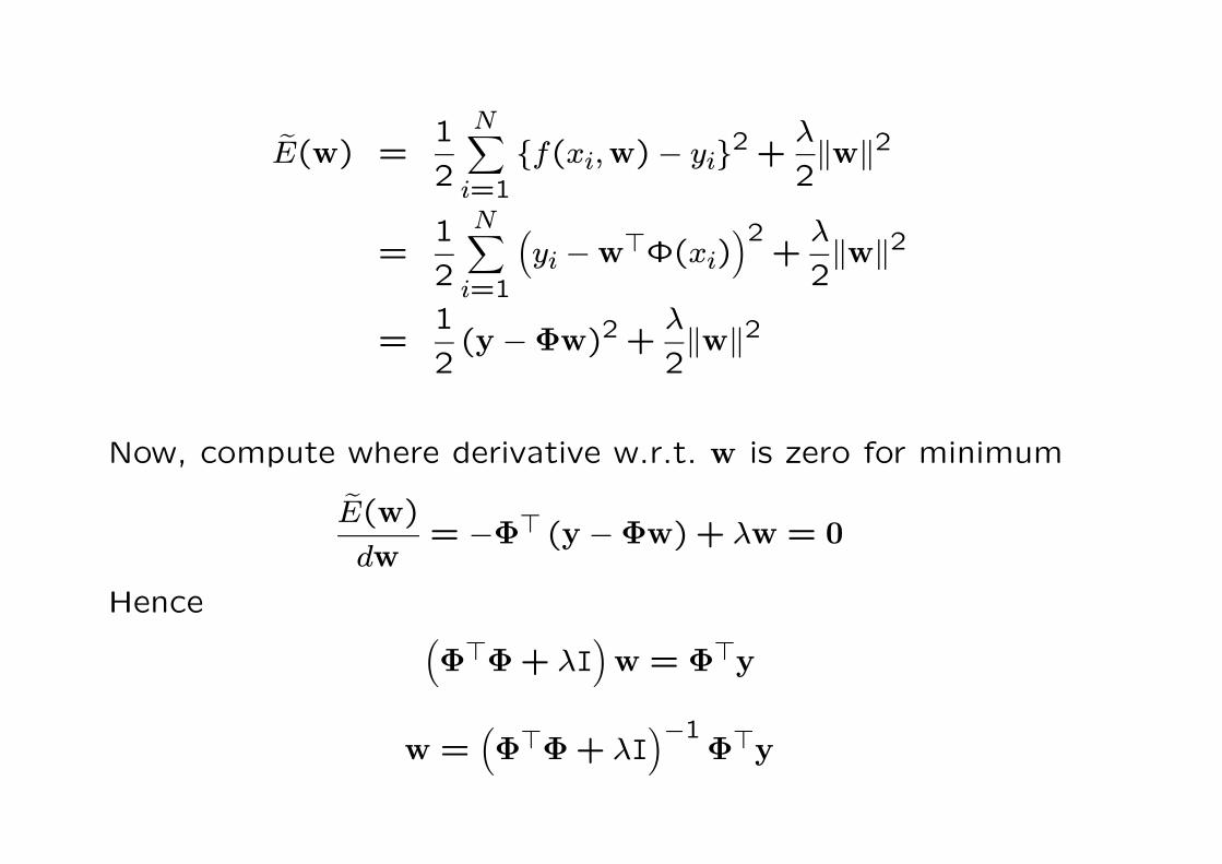
eE(w) =1

2

NXi=1

{f(xi,w)− yi}2 +λ

2kwk2

=1

2

NXi=1

³yi −w>Φ(xi)

´2+

λ

2kwk2

=1

2(y −Φw)2 + λ

2kwk2

Now, compute where derivative w.r.t. w is zero for minimum

eE(w)dw

= −Φ> (y −Φw) + λw = 0

Hence ³Φ>Φ+ λI

´w = Φ>y

w =³Φ>Φ+ λI

´−1Φ>y

w =³Φ>Φ+ λI

´−1Φ>y

= assume N > M

M x 1 M x M

M basis functions, N data points

M x N N x 1

• This shows that there is a unique solution.

• If λ = 0 (no regularization), then

w = (Φ>Φ )−1Φ>y = Φ+y

where Φ+ is the pseudo-inverse of Φ (pinv in Matlab)

• Adding the term λI improves the conditioning of the inverse, since if Φ

is not full rank, then (Φ>Φ+ λI) will be (for sufficiently large λ)

• As λ→∞, w→ 1λΦ

>y→ 0

• Often the regularization is applied only to the inhomogeneous part of w,i.e. to w, where w = (w0, w)

w =³Φ>Φ+ λI

´−1Φ>y

f(x,w) = w>Φ(x) = Φ(x)>w

= Φ(x)>³Φ>Φ+ λI

´−1Φ>y

= b(x)>y

Output is a linear blend, b(x), of the training values {yi}

0 0.1 0.2 0.3 0.4 0.5 0.6 0.7 0.8 0.9 1-1.5

-1

-0.5

0

0.5

1

1.5

x

y

ideal fit

Sample pointsIdeal fit

Example 1: polynomial basis functions

• The red curve is the true function (which is not a polynomial)

• The data points are samples from the curve with added noise in y.

• There is a choice in both the degree, M, of the basis functions used, and in the strength of the regularization

f(x,w) =MXj=0

wjxj = w>Φ(x)

w is a M+1 dimensional vector

Φ : x→ Φ(x) R→ RM+1

0 0.1 0.2 0.3 0.4 0.5 0.6 0.7 0.8 0.9 1-1.5

-1

-0.5

0

0.5

1

1.5

x

y

Sample pointsIdeal fitlambda = 100

0 0.1 0.2 0.3 0.4 0.5 0.6 0.7 0.8 0.9 1-1.5

-1

-0.5

0

0.5

1

1.5

x

y

Sample pointsIdeal fitlambda = 0.001

0 0.1 0.2 0.3 0.4 0.5 0.6 0.7 0.8 0.9 1-1.5

-1

-0.5

0

0.5

1

1.5

x

y

Sample pointsIdeal fitlambda = 1e-010

0 0.1 0.2 0.3 0.4 0.5 0.6 0.7 0.8 0.9 1-1.5

-1

-0.5

0

0.5

1

1.5

x

y


N = 9 samples, M = 7

0 0.1 0.2 0.3 0.4 0.5 0.6 0.7 0.8 0.9 1

-25

-20

-15

-10

-5

0

5

10

15

x

y

Polynomial basis functions

M = 3

0 0.1 0.2 0.3 0.4 0.5 0.6 0.7 0.8 0.9 1-1.5

-1

-0.5

0

0.5

1

1.5

x

y

least-squares fit

Sample pointsIdeal fitLeast-squares solution

0 0.1 0.2 0.3 0.4 0.5 0.6 0.7 0.8 0.9 1

-400

-300

-200

-100

0

100

200

300

400

x

y

Polynomial basis functions

M = 5

0 0.1 0.2 0.3 0.4 0.5 0.6 0.7 0.8 0.9 1-1.5

-1

-0.5

0

0.5

1

1.5

x

y

least-squares fit

Sample pointsIdeal fitLeast-squares solution

0 0.1 0.2 0.3 0.4 0.5 0.6 0.7 0.8 0.9 1-1.5

-1

-0.5

0

0.5

1

1.5

x

y

ideal fit

Sample pointsIdeal fit

Example 2: Gaussian basis functions

• The red curve is the true function (which is not a polynomial)• The data points are samples from the curve with added noise in y.

• Basis functions are centred on the training data (N points)• There is a choice in both the scale, sigma, of the basis functions used, and in the strength of the regularization

f(x,w) =NXi=1

wie−(x−xi)2/σ2 = w>Φ(x)

w is a N-vector

Φ : x→ Φ(x) R→ RN

N = 9 samples, sigma = 0.334

0 0.1 0.2 0.3 0.4 0.5 0.6 0.7 0.8 0.9 1-1.5

-1

-0.5

0

0.5

1

1.5

x

y

Sample pointsIdeal fitlambda = 100

0 0.1 0.2 0.3 0.4 0.5 0.6 0.7 0.8 0.9 1-1.5

-1

-0.5

0

0.5

1

1.5

x

y

Sample pointsIdeal fitlambda = 0.001

0 0.1 0.2 0.3 0.4 0.5 0.6 0.7 0.8 0.9 1-1.5

-1

-0.5

0

0.5

1

1.5

x

y


0 0.1 0.2 0.3 0.4 0.5 0.6 0.7 0.8 0.9 1-1.5

-1

-0.5

0

0.5

1

1.5

x

y


10-10 10-5 1000

1

2

3

4

5

6

log

erro

r nor

m

Ideal fitValidationTrainingMin error

0 0.1 0.2 0.3 0.4 0.5 0.6 0.7 0.8 0.9 1-1.5

-1

-0.5

0

0.5

1

1.5

x

y

Sample pointsIdeal fitValidation set fit

Choosing lambda using a validation set

0 0.1 0.2 0.3 0.4 0.5 0.6 0.7 0.8 0.9 1-1.5

-1

-0.5

0

0.5

1

1.5

x

y


0 0.1 0.2 0.3 0.4 0.5 0.6 0.7 0.8 0.9 1

-0.8

-0.6

-0.4

-0.2

0

0.2

0.4

0.6

0.8

x

y

Gaussian basis functions

Sigma = 0.1

0 0.1 0.2 0.3 0.4 0.5 0.6 0.7 0.8 0.9 1-1.5

-1

-0.5

0

0.5

1

1.5

x

y


0 0.1 0.2 0.3 0.4 0.5 0.6 0.7 0.8 0.9 1

-2000

-1500

-1000

-500

0

500

1000

1500

2000

x

y

Gaussian basis functions

Sigma = 0.334

Application: regressing face pose

• Estimate two face pose angles: • yaw (around the Y axis)

• pitch (around the X axis)

• Compute a HOG feature vector for each face region

• Learn a regressor from the HOG vector to the two pose angles

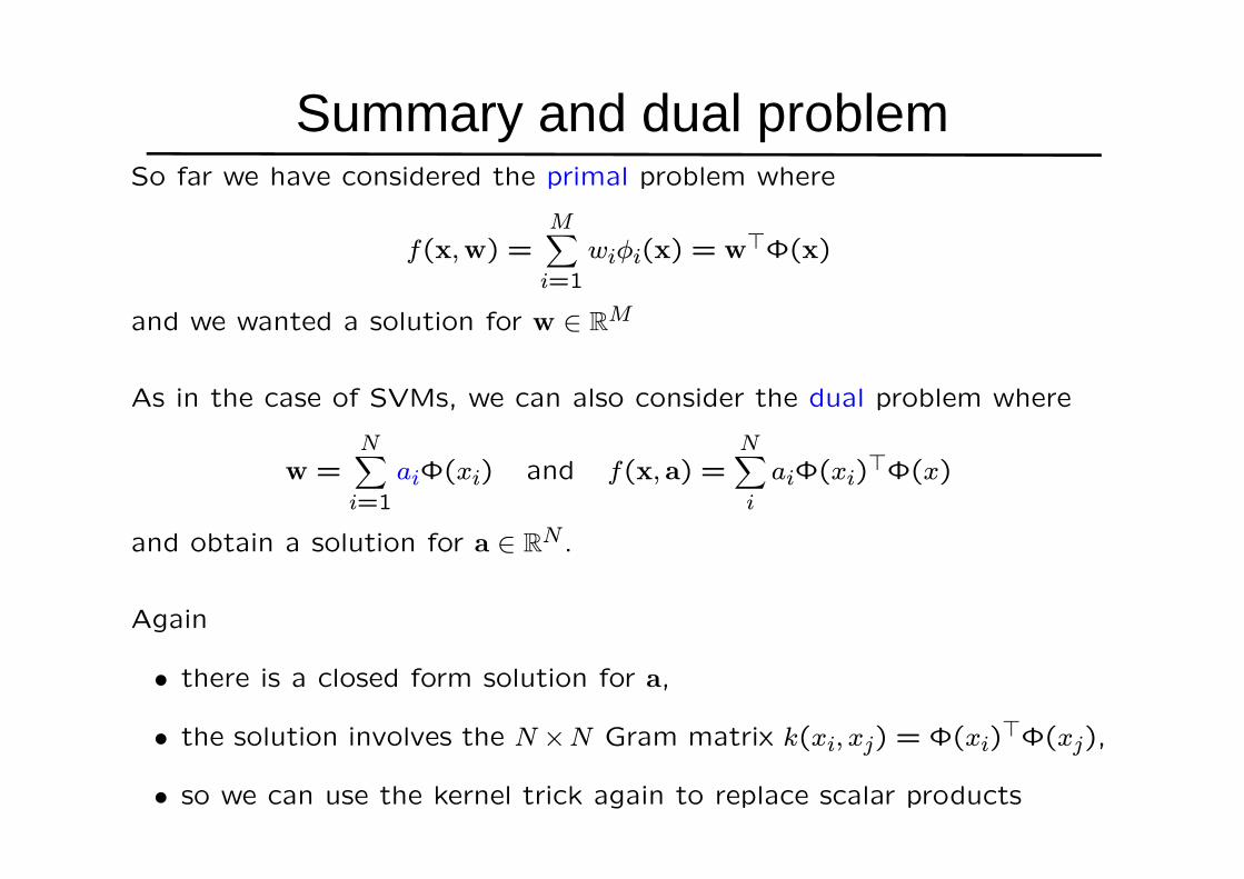
Summary and dual problemSo far we have considered the primal problem where

f(x,w) =MXi=1

wiφi(x) = w>Φ(x)

and we wanted a solution for w ∈ RM

As in the case of SVMs, we can also consider the dual problem where

w =NXi=1

aiΦ(xi) and f(x, a) =NXi

aiΦ(xi)>Φ(x)

and obtain a solution for a ∈ RN .

Again

• there is a closed form solution for a,

• the solution involves the N ×N Gram matrix k(xi, xj) = Φ(xi)>Φ(xj),

• so we can use the kernel trick again to replace scalar products

Background reading and more

• Bishop, chapters 6 & 7 for kernels and SVMs

• Hastie et al, chapter 12

• Bishop, chapter 3 for regression

• More on web page: http://www.robots.ox.ac.uk/~az/lectures/ml

lecture 3: svm dual, kernels and multiple classes

Documents