lecture 3: measure of central tendency - unbddu/2623/lecture_notes/lecture3_student.pdf · table of...
TRANSCRIPT

Lecture 3: Measure of Central Tendency
Donglei Du([email protected])
Faculty of Business Administration, University of New Brunswick, NB Canada FrederictonE3B 9Y2
Donglei Du (UNB) ADM 2623: Business Statistics 1 / 53
Table of contents
1 Measure of central tendency: location parameterIntroductionArithmetic MeanWeighted Mean (WM)MedianModeGeometric MeanMean for grouped dataThe Median for Grouped DataThe Mode for Grouped Data
2 Dicussion: How to lie with averges? Or how to defend yourselves fromthose lying with averages?
Donglei Du (UNB) ADM 2623: Business Statistics 2 / 53

Section 1
Measure of central tendency: location parameter
Donglei Du (UNB) ADM 2623: Business Statistics 3 / 53
Subsection 1
Introduction
Donglei Du (UNB) ADM 2623: Business Statistics 4 / 53
Introduction
Characterize the average or typical behavior of the data.
There are many types of central tendency measures:
Arithmetic meanWeighted arithmetic meanGeometric meanMedianMode
Donglei Du (UNB) ADM 2623: Business Statistics 5 / 53

Subsection 2
Arithmetic Mean
Donglei Du (UNB) ADM 2623: Business Statistics 6 / 53

Arithmetic Mean
The Arithmetic Mean of a set of n numbers
AM =x1 + . . .+ xn
n
Arithmetic Mean for population and sample
µ =
N∑i=1
xi
N
x̄ =
n∑i=1
xi
n
Donglei Du (UNB) ADM 2623: Business Statistics 7 / 53
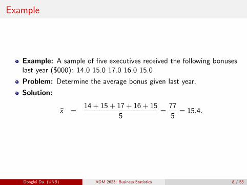
Example
Example: A sample of five executives received the following bonuseslast year ($000): 14.0 15.0 17.0 16.0 15.0
Problem: Determine the average bonus given last year.
Solution:
x̄ =14 + 15 + 17 + 16 + 15
5=
77
5= 15.4.
Donglei Du (UNB) ADM 2623: Business Statistics 8 / 53
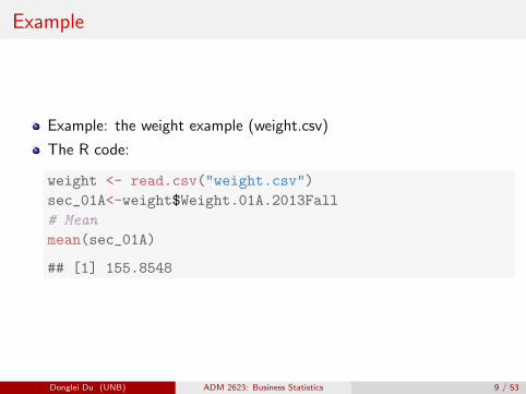
Example
Example: the weight example (weight.csv)
The R code:
weight <- read.csv("weight.csv")
sec_01A<-weight$Weight.01A.2013Fall
# Mean
mean(sec_01A)
## [1] 155.8548
Donglei Du (UNB) ADM 2623: Business Statistics 9 / 53

Will Rogers phenomenon
Consider two sets of IQ scores of famous people.
Group 1 IQ Group 2 IQ
Albert Einstein 160 John F. Kennedy 117Bill Gates 160 George Washington 118
Sir Isaac Newton 190 Abraham Lincoln 128
Mean 170 Mean 123
Let us move Bill Gates from the first group to the second group
Group 1 IQ Group 2 IQ
Albert Einstein 160 John F. Kennedy 117Bill Gates 160
Sir Isaac Newton 190 George Washington 118Abraham Lincoln 128
Mean 175 Mean 130.75
Donglei Du (UNB) ADM 2623: Business Statistics 10 / 53
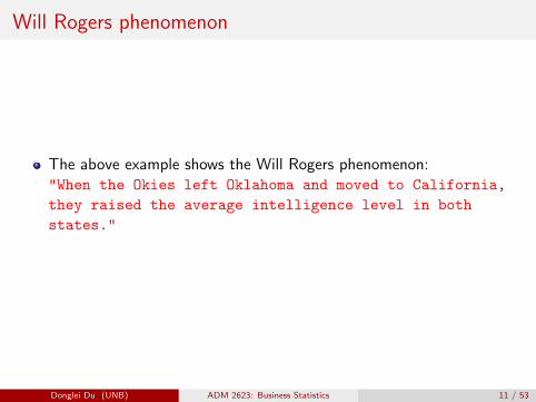
Will Rogers phenomenon
The above example shows the Will Rogers phenomenon:"When the Okies left Oklahoma and moved to California,
they raised the average intelligence level in both
states."
Donglei Du (UNB) ADM 2623: Business Statistics 11 / 53
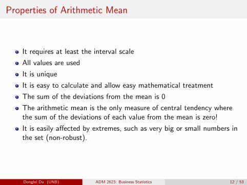
Properties of Arithmetic Mean
It requires at least the interval scale
All values are used
It is unique
It is easy to calculate and allow easy mathematical treatment
The sum of the deviations from the mean is 0
The arithmetic mean is the only measure of central tendency wherethe sum of the deviations of each value from the mean is zero!
It is easily affected by extremes, such as very big or small numbers inthe set (non-robust).
Donglei Du (UNB) ADM 2623: Business Statistics 12 / 53

The sum of the deviations from the mean is 0: anillustration
Values deviations
3 -24 -18 3
Mean 5 0
Donglei Du (UNB) ADM 2623: Business Statistics 13 / 53

How Extremes Affect the Arithmetic Mean?
The mean of the values 1,1,1,1,100 is 20.8.
However, 20.8 does not represent the typical behavior of this data set!
Extreme numbers relative to the rest of the data is called outliers!
Examination of data for possible outliers serves many useful purposes,including
Identifying strong skew in the distribution.Identifying data collection or entry errors.Providing insight into interesting properties of the data.
Donglei Du (UNB) ADM 2623: Business Statistics 14 / 53
Subsection 3
Weighted Mean (WM)
Donglei Du (UNB) ADM 2623: Business Statistics 15 / 53

Weighted Mean (WM)
The Weighted Mean (WM) of a set of n numbers
WM =w1x1 + . . .+ wnxnw1 + . . .+ wn
This formula will be used to calculate the mean and variance forgrouped data!
Donglei Du (UNB) ADM 2623: Business Statistics 16 / 53

Example
Example: During an one hour period on a hot Saturday afternoonCabana boy Chris served fifty drinks. He sold:
five drinks for $0.50fifteen for $0.75fifteen for $0.90fifteen for $1.10
Problem: compute the weighted mean of the price of the drinks
WM =5(0.50) + 15(0.75) + 15(0.90) + 15(1.10)
5 + 15 + 15 + 15=
43.75
50= 0.875.
Donglei Du (UNB) ADM 2623: Business Statistics 17 / 53

Example
Example: the above example
The R code:
## weighted mean
wt <- c(5, 15, 15, 15)/50
x <- c(0.5,0.75,0.90,1.1)
weighted.mean(x, wt)
## [1] 0.875
Donglei Du (UNB) ADM 2623: Business Statistics 18 / 53

Subsection 4
Median
Donglei Du (UNB) ADM 2623: Business Statistics 19 / 53

Median
The Median is the midpoint of the values after they have beenordered from the smallest to the largest
Equivalently, the Median is a number which divides the data set intotwo equal parts, each item in one part is no more than this number,and each item in another part is no less than this number.
Donglei Du (UNB) ADM 2623: Business Statistics 20 / 53

Two-step process to find the median
Step 1. Sort the data in a nondecreasing order
Step 2. If the total number of items n is an odd number, thenthe number on the (n+1)/2 position is the median;If n is an even number, then the average of the twonumbers on the n/2 and n/2+1 positions is the median.(For ordinal level of data, choose any one on the twomiddle positions).
Donglei Du (UNB) ADM 2623: Business Statistics 21 / 53

Examples
Example: The ages for a sample of five college students are: 21, 25,19, 20, 22
Arranging the data in ascending order gives: 19, 20, 21, 22, 25.
The median is 21.
Example: The heights of four basketball players, in inches, are: 76,73, 80, 75
Arranging the data in ascending order gives: 73, 75, 76, 80. Themedian is the average of the two middle numbers
Median =75 + 76
2= 75.5.
Donglei Du (UNB) ADM 2623: Business Statistics 22 / 53

One more example
Example: Earthquake intensities are measured using a device called aseismograph which is designed to be most sensitive for earthquakeswith intensities between 4.0 and 9.0 on the open-ended Richter scale.Measurements of nine earthquakes gave the following readings:
4.5, L, 5.5, H, 8.7, 8.9, 6.0, H, 5.2
where L indicates that the earthquake had an intensity below 4.0 anda H indicates that the earthquake had an intensity above 9.0.
Problem: What is the median earthquake intensity of the sample?
Solution:Step 1. Sort: L, 4.5, 5.2, 5.5, 6.0, 8.7, 8.9, H, HStep 2. So the median is 6.0
Donglei Du (UNB) ADM 2623: Business Statistics 23 / 53
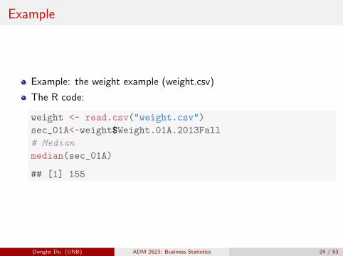
Example
Example: the weight example (weight.csv)
The R code:
weight <- read.csv("weight.csv")
sec_01A<-weight$Weight.01A.2013Fall
# Median
median(sec_01A)
## [1] 155
Donglei Du (UNB) ADM 2623: Business Statistics 24 / 53

Properties of Median
It requires at least the ordinal scale
All values are used
It is unique
It is easy to calculate but does not allow easy mathematical treatment
It is not affected by extremely large or small numbers (robust)
Donglei Du (UNB) ADM 2623: Business Statistics 25 / 53
Subsection 5
Mode
Donglei Du (UNB) ADM 2623: Business Statistics 26 / 53

Mode
The number that has the highest frequency.
Donglei Du (UNB) ADM 2623: Business Statistics 27 / 53

Example
Example: The exam scores for ten students are: 81, 93, 84, 75, 68,87, 81, 75, 81, 87
The score of 81 occurs the most often. It is the Mode!
Donglei Du (UNB) ADM 2623: Business Statistics 28 / 53
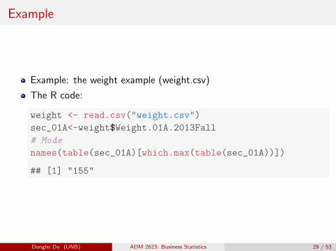
Example
Example: the weight example (weight.csv)
The R code:
weight <- read.csv("weight.csv")
sec_01A<-weight$Weight.01A.2013Fall
# Mode
names(table(sec_01A)[which.max(table(sec_01A))])
## [1] "155"
Donglei Du (UNB) ADM 2623: Business Statistics 29 / 53

Properties of Mode
Even nominal data have mode(s)
All values are used
It is not unique
Modeless: if all data have different values, such as 1,1,1Multimodal: if more than one value have the same frequency, such as1,1,2,2,3.
It is easy to calculate but does not allow easy mathematical treatment
It is not affected by extremely large or small numbers (robust)
Donglei Du (UNB) ADM 2623: Business Statistics 30 / 53

Subsection 6
Geometric Mean
Donglei Du (UNB) ADM 2623: Business Statistics 31 / 53
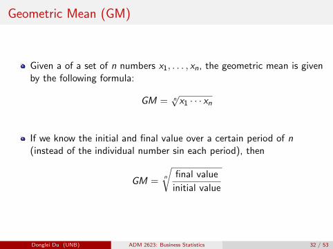
Geometric Mean (GM)
Given a of a set of n numbers x1, . . . , xn, the geometric mean is givenby the following formula:
GM = n√x1 · · · xn
If we know the initial and final value over a certain period of n(instead of the individual number sin each period), then
GM =n
√final value
initial value
Donglei Du (UNB) ADM 2623: Business Statistics 32 / 53

Example
Example: The interest rate on three bonds was 5%, 21%, and 4%percent. Suppose you invested $10000 at the beginning on the firstbond, then switch to the second bond in the following year, andswitch again to the third bond the next year.
Problem: What is your final wealth after three years?
Solution:Your final wealth will be
10000× GM3 = 10, 000× 1.0973 = 13213.2,
whereGM = 3
√1.05× 1.21× 1.04 ≈ 1.097
Donglei Du (UNB) ADM 2623: Business Statistics 33 / 53
Example
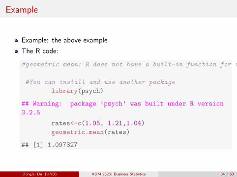
Example: the above example
The R code:
#geometric mean: R does not have a built-in function for this.
#You can install and use another package
library(psych)
## Warning: package ’psych’ was built under R version
3.2.5
rates<-c(1.05, 1.21,1.04)
geometric.mean(rates)
## [1] 1.097327
Donglei Du (UNB) ADM 2623: Business Statistics 34 / 53

Example
Example: The total number of females enrolled in American collegesincreased from 755,000 in 1992 to 835,000 in 2000.
Problem: What is your the geometric mean rate of increase?.
Solution:The geometric mean over these 8 years is
GM = 8
√835, 000
755, 000≈ 1.0127.
Therefore the geometric mean rate of increase is 1.27%.
Donglei Du (UNB) ADM 2623: Business Statistics 35 / 53

Arithmetic Mean vs Geometric Mean: the AM-GMinequality:
If x1, . . . , xn ≥ 0, then
AM =x1 + x2 + · · ·+ xn
n≥ n√x1x2 . . . xn = GM,
with equality if and only if x1 = x2 = · · · = xn.
Donglei Du (UNB) ADM 2623: Business Statistics 36 / 53

Arithmetic Mean vs Geometric Mean: the AM-GMinequality:
If x1, . . . , xn ≥ 0, then
AM =x1 + x2 + · · ·+ xn
n≥ n√x1x2 . . . xn = GM,
with equality if and only if x1 = x2 = · · · = xn.
Donglei Du (UNB) ADM 2623: Business Statistics 37 / 53

Case: GM vs AM in fund reporting
A fund manager tries to convince you to invest in their fund byshowing you the annual returns over the last five years
10%,−20%, 30%, 12%, 10%
and the average return per year realized in the last five years is 8.4%as calculated as follows.
AM =(1 + 0.1) + (1− 0.2) + (1 + 0.3) + (1 + 0.12) + (1 + 0.1)
5= 1.084
This is misleading sometimes. It is much better to say that theaverage return realized over the last fives with us is approximately 7%per year:
GM = 5√
1.10× 0.80× 1.30× 1.12× 1.10− 1 ≈ 0.07104408
Donglei Du (UNB) ADM 2623: Business Statistics 38 / 53
Example
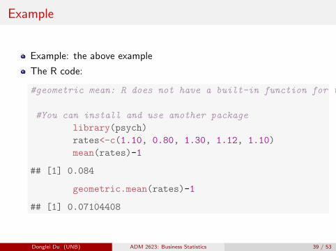
Example: the above example
The R code:
#geometric mean: R does not have a built-in function for this.
#You can install and use another package
library(psych)
rates<-c(1.10, 0.80, 1.30, 1.12, 1.10)
mean(rates)-1
## [1] 0.084
geometric.mean(rates)-1
## [1] 0.07104408
Donglei Du (UNB) ADM 2623: Business Statistics 39 / 53

Properties of Geometric Mean
Similar to arithmetic mean, except used in different scenario
It requires interval level
All values are used
It is unique
It is easy to calculate and allow easy mathematical treatments
Donglei Du (UNB) ADM 2623: Business Statistics 40 / 53

Subsection 7
Mean for grouped data
Donglei Du (UNB) ADM 2623: Business Statistics 41 / 53
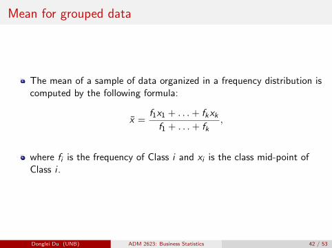
Mean for grouped data
The mean of a sample of data organized in a frequency distribution iscomputed by the following formula:
x̄ =f1x1 + . . .+ fkxkf1 + . . .+ fk
,
where fi is the frequency of Class i and xi is the class mid-point ofClass i .
Donglei Du (UNB) ADM 2623: Business Statistics 42 / 53

Example
Example: Recall the weight example from Chapter 2:
class freq. (fi ) mid point (xi ) fixi[130, 140) 3 135 405
[140, 150) 12 145 1740
[150, 160) 23 155 3565
[160, 170) 14 165 2310
[170, 180) 6 175 1050
[180, 190] 4 185 740
62 9810
The mean for the grouped data is:
x̄ =9810
62≈ 158.2258.
The real mean for the raw data is 155.8548.
Donglei Du (UNB) ADM 2623: Business Statistics 43 / 53

Subsection 8
The Median for Grouped Data
Donglei Du (UNB) ADM 2623: Business Statistics 44 / 53

Median for grouped data: Two-step procedure
Step 1: identify the median class, which is the class that contains thenumber on the n/2 position.
Step 2: Estimate the median value within the median class using thefollowing formula:
median = L + C ×n2 − CF
f,
where
L is the lower limit of the median classCF is the cumulative frequency before the median classf is the frequency of the median classC is the class interval or size
Donglei Du (UNB) ADM 2623: Business Statistics 45 / 53

Example
Example: Recall the weight example from Chapter 2:
class freq relative freq. cumulative freq.
[130, 140) 3 0.05 3
[140, 150) 12 0.19 15
[
10︷ ︸︸ ︷150, 160) 23 0.37 38
[160, 170) 14 0.23 52
[170, 180) 6 0.10 58
[180, 190] 4 0.06 62
median = 150 + 10×622 − 15
23≈ 156.9565.
Donglei Du (UNB) ADM 2623: Business Statistics 46 / 53

An explanation of the median formula
CF 2n
1 2 3L U
CF 2
f
C
Donglei Du (UNB) ADM 2623: Business Statistics 47 / 53
Subsection 9
The Mode for Grouped Data
Donglei Du (UNB) ADM 2623: Business Statistics 48 / 53
Mode for grouped data: Two-step procedure
Step 1: Identify the modal class, which is the class(es) that has thehighest frequency(ies).
Step 2: Estimate the modal(s) within the modal class (es) as theclass midpoint(s).
Donglei Du (UNB) ADM 2623: Business Statistics 49 / 53

Example
Example: Recall the weight example from Chapter 2:
class freq. (fi ) mid point (xi )
[130, 140) 3 135
[140, 150) 12 145
[150, 160) 23 155
[160, 170) 14 165
[170, 180) 6 175
[180, 190] 4 185
mode = 155.
Donglei Du (UNB) ADM 2623: Business Statistics 50 / 53

Section 2
Dicussion: How to lie with averges? Or how to defendyourselves from those lying with averages?
Donglei Du (UNB) ADM 2623: Business Statistics 51 / 53

Lie with averages
There are many different interpreations of averages:
Arithemtic Mean vs Geometric mean: be careful of investment fundstatementsMean vs Median: be careful of the accounting statements
[Huff, 2010]
Donglei Du (UNB) ADM 2623: Business Statistics 52 / 53

References I
Huff, D. (2010).How to lie with statistics.WW Norton & Company.
Donglei Du (UNB) ADM 2623: Business Statistics 53 / 53