lecture 3 lossless source coding -...

Typical Sequences and a Lossless Source Coding TheoremWeakly Typical Sequences and Sources with Memory

Lecture 3Lossless Source Coding

I-Hsiang Wang

Department of Electrical EngineeringNational Taiwan University

[email protected]

September 25, 2015

1 / 47 I-Hsiang Wang IT Lecture 3

[email protected]


The Source Coding Problem

Source Encoder

Source DecoderSource Destination

s[1 : N ] b[1 : K] bs[1 : N ]

Meta Description

1 Encoder:Represent the source sequence s[1 : N] by a binary source codewordw ≜ b[1 : K] ∈

{0, 1, . . . , 2K − 1

}, with K as small as possible.

2 Decoder:From the source codeword w, reconstruct the source sequence eitherlosslessly or within a certain distortion.

3 Efficiency:Determined by the code rate R ≜ K

N bits/symbol time



Decoding Criteria

Source Encoder


s[1 : N ] b[1 : K] bs[1 : N ]

Naturally, one would think of two different decoding criteria for thesource coding problem.

1 Exact: the reconstructed sequence s[1 : N] = s[1 : N].2 Lossy: the reconstructed sequence s[1 : N] = s[1 : N], but is within a

prescribed distortion.



Let us begin with some simple analysis of the system with the exactrecovery criterion.For N fixed, if the decoder would like to reconstruct s[1 : N] exactly forall possible s[1 : N] ∈ SN, then it is simple to see that the smallest Kmust satisfy

2K−1 < |S|N ≤ 2K =⇒ K = ⌈N log |S|⌉.

Why?Because every possible sequence has to be uniquely represented by K bits!As a consequence, it seems that if we require exact reconstruction, it isimpossible to have data compression.

What is going wrong?



Random Source

Recall: data compression is possible because there is redundancy in thesource sequence.One of the simplest ways to capture redundancy is to model the sourceas a random process. (Another reason to use a random source model is due toengineering reasons, as mentioned in Lecture 1.)

Redundancy comes from the fact that different symbols in S takedifferent probabilities to be drawn.With a random source model, immediately there are two approaches onecan take to demonstrate data compression:

Allow variable codeword length for different symbols with differentprobabilities, rather than fixing it to be KAllow (almost) lossless reconstruction rather than exact recovery



Block-to-Variable Source Coding

b[1 : K]Source

EncoderSource

DecoderSource Destination

s[1 : N ] bs[1 : N ]

Variable Length

The key difference here is that we allow K to depend on the realization ofthe source, s[1 : N].Using variable codeword length is intuitive – for symbols with higherprobability, we tend to use shorter codewords to represent it.

The definition of the code rate is modified to R ≜ E[K]N .

In a later lecture on Data Compression, we will introduce an optimalblock-to-variable source code, Huffman code, which can achieve theminimum compression rate for a given distribution of the random source.Note: the decoding criterion here is exact reconstruction.



(Almost) Lossless Decoding Criterion

Another way to let the randomness kick in: allow non-exact recovery.To be precise, we turn our focus to finding the smallest possible R = K

Ngiven that the error probability

P(N)e ≜ P

{S[1 : N] = S[1 : N]

}→ 0 as N→∞.

Key features of this approach:

Focus on the asymptotic regime where N→∞; instead of error-freereconstruction, the criterion is relaxed to vanishing error probability.Compared to the previous approach where the analysis is mainlycombinatorial, the analysis here is majorly probabilistic.



Outline

In this lecture, we shall

1 First, focusing on memoryless sources, introduce a powerful toolcalled typical sequences, and use typical sequences to prove alossless source coding theorem

2 Second, extend the typical sequence framework to sources withmemory, and prove a similar lossless source coding theorem there.

We will show that the minimum compression rate is equal to the entropyof the random source.Let us begin with the simplest case where the source {S[t] | t = 1, 2, . . .}consists of i.i.d. random variables S[t] i.i.d.∼ pS, which is called a discretememoryless source (DMS).



Typicality and AEPLossless Source Coding Theorem

1 Typical Sequences and a Lossless Source Coding TheoremTypicality and AEPLossless Source Coding Theorem

2 Weakly Typical Sequences and Sources with MemoryEntropy Rate of Random ProcessesTypicality for Sources with Memory




Overview of Typicality Methods

Goal: Understand and exploit the probabilistic asymptotic properties of ai.i.d. randomly generated sequence S[1 : N] for coding.Key Observation: When N→∞, one often observe that a substantiallysmall set of sequences become “typical”, which contribute almost thewhole probability, while others become “atypical”.(cf. Lecture 2 “Operational Meaning of Entropy”)

For lossless reconstruction with vanishing error probability, we can useshorter codewords to label “typical” sequences and ignore “atypical” ones.Note: There are several notions of typicality and various definitions inthe literature. In this lecture, we give two definitions: (robust) typicalityand weak typicality.Notation: For notational convenience, we shall use the followinginterchangeably: x[t]←→ xt, and x[1 : N]←→ xN.




Typical Sequence

Roughly speaking, a (robust) typical sequence is a sequence whoseempirical distribution is close to the actual distribution.For a sequence xn, its empirical p.m.f. is given by the frequency ofoccurrence of a symbol in the sequence: π (a|xn) ≜

∑ni=1 1{xi=a}

n .

Due the law of large numbers, π (a|xn)p→ pX (a) for all a ∈ X as

n→∞, if xn is drawn i.i.d. based on pX. With high probability, theempirical p.m.f. does not deviate too much from the actual p.m.f.

Definition 1 (Typical Sequence)For X ∼ pX and ε ∈ (0, 1), a sequence xn is called ε-typical if|π (a|xn)− pX (a)| ≤ εpX (a) , ∀ a ∈ X .The typical set is defined as the collection of all ε-typical length-nsequences, denoted by T (n)

ε (X).




Note: In the following, if the context is clear, we will write “T (n)ε ”

instead of “T (n)ε (X)”.

Example 1Consider a random bit sequence generated i.i.d. based on Ber

( 12). Let

us set ε = 0.2 and n = 10. What is T (n)ε ? How large is the typical set?

sol: Based on the definition, a n-sequence xn is ε-typical iff

π (0|xn) ∈ [0.4, 0.6] and π (1|xn) ∈ [0.4, 0.6].

In other words, the # of “0”s in the sequence should be 4, 5, or 6.Hence, T (n)

ε consists of all length-10 sequences with 4, 5, or 6 0”s.

The size of T (n)ε is

(104

)+(105

)+

(106

)= 714.




Properties of Typical Sequences

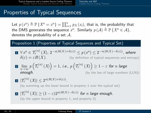
Let p (xn) ≜ P {Xn = xn} =∏n

i=1 pX (xi), that is, the probability thatthe DMS generates the sequence xn. Similarly p (A) ≜ P {Xn ∈ A},denotes the probability of a set A.

Proposition 1 (Properties of Typical Sequences and Typical Set)

1 ∀ xn ∈ T (n)ε (X), 2−n(H(X )+δ(ε)) ≤ p (xn) ≤ 2−n(H(X )−δ(ε)), where

δ(ε) = εH (X ). (by definition of typical sequences and entropy)

2 limn→∞

p(T (n)ε (X)

)= 1, i.e., p

(T (n)ε (X)

)≥ 1− ε for n large

enough. (by the law of large numbers (LLN))

3 |T (n)ε (X)| ≤ 2n(H(X )+δ(ε)).

(by summing up the lower bound in property 1 over the typical set)

4 |T (n)ε (X)| ≥ (1− ε)2n(H(X )−δ(ε)) for n large enough.

(by the upper bound in property 1, and property 2)




Asymptotic Equipartition Property (AEP)

Xn T (n)� (X)

p�T (n)

� (X)�

� 1

|T (n)� (X)| � 2nH(X)

typical xn

p (xn) ⇡ 2�nH(X)

Observation:1 The typical set has probability approach 1 as n→∞, while its size is

roughly equal to 2nH(X ), significantly smaller than |X n| = 2n log|X |.2 Within the typical set, all typical sequences have roughly the same

probability 2−nH(X ).




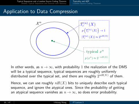
Application to Data Compression

Xn T (n)� (X)

p�T (n)

� (X)�

� 1

|T (n)� (X)| � 2nH(X)

typical xn

p (xn) ⇡ 2�nH(X)

In other words, as n→∞, with probability 1 the realization of the DMSwill be a typical sequence, typical sequences are roughly uniformlydistributed over the typical set, and there are roughly 2nH(X ) of them.Hence, we can use roughly nH (X ) bits to uniquely describe each typicalsequence, and ignore the atypical ones. Since the probability of gettingan atypical sequence vanishes as n→∞, so does error probability.




Lossless Source Coding: Problem Setup

Source Encoder


s[1 : N ] b[1 : K] bs[1 : N ]

1 A(2NR,N

)lossless source code consists of

an encoding function (encoder) encN : SN → {0, 1}K that mapseach source sequence sN to a bit sequence bK, where K ≜ ⌊NR⌋.a decoding function (decoder) decN : {0, 1}K → SN that maps eachbit sequence bK to a reconstructed source sequence sN.

2 The error probability for a(2NR,N

)lossless source code is defined

as P(N)e ≜ P

{SN = SN

}.

3 A rate R is said to be achievable if there exist a sequence of(2NR,N

)codes such that P(N)

e → 0 as N→∞. The optimalcompression rate R∗ ≜ inf {R | R : achievable}.




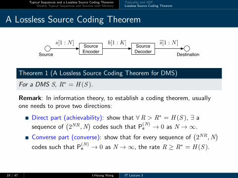
A Lossless Source Coding Theorem

Source Encoder


s[1 : N ] b[1 : K] bs[1 : N ]

Theorem 1 (A Lossless Source Coding Theorem for DMS)For a DMS S, R∗ = H (S ).

Remark: In information theory, to establish a coding theorem, usuallyone needs to prove two directions:

Direct part (achievability): show that ∀R > R∗ = H (S ), ∃ asequence of

(2NR,N


e → 0 as N→∞.Converse part (converse): show that for every sequence of

(2NR,N


e → 0 as N→∞, the rate R ≥ R∗ = H (S ).




Lossless Source Coding Theorem: Achievability Proof (1)

Source Encoder


s[1 : N ] b[1 : K] bs[1 : N ]

pf: Here we provide a simple proof based on typical sequences.Codebook Generation: Let us choose an ε > 0 and set R = H (S ) + δ (ε)such that NR ∈ Z, where δ (ε) = εH (S ). By property 3 of Proposition 1, wehave an upper bound on the # of typical sequences:|T (N)

ε (S)| ≤ 2N(H(S )+δ(ε)) = 2NR.

Encoding: Hence, we are able to label each typical sequence with a length NRbit sequence, which defines the encoding function ∀ sN ∈ T (N)

ε . For sN /∈ T (N)ε ,

the encoding function maps them to the all 0 sequence.

Decoding: The decoding function simply maps the received bit sequence backto the typical sequence labeled by the bit sequence.




Lossless Source Coding Theorem: Achievability Proof (2)

Source Encoder


s[1 : N ] b[1 : K] bs[1 : N ]

Error Probability Analysis: Obviously an error occurs iff the generatedsequence sN /∈ T (N)

ε , since all typical sequence can be reconstructed uniquelyand perfectly. Hence,

P(N)e ≤ P(N)

e ≜ P{

SN /∈ T (N)ε

}= 1− p

(T (N)ε

)→ 1− 1 = 0 as N → ∞,

due to property 2 of Proposition 1.

Finally, since δ (ε) can be made arbitrarily small, we have shown that∀R > R∗ = H (S ), ∃ a sequence of

(2NR,N


e → 0 asN → ∞.




Reflections

In proving the achievability, essentially we give an upper bound on P(N)e

for some coding scheme; by asserting that the upper bound → 0 asN→ 0, we show that the rate of the coding scheme is achievable.For the achievability of the lossless source coding problem, indeed we findan upper bound for the error probability – note that the typicalityencoder needs not be optimal. Hence, the optimal probability of errorP(N)

e ≤ P(N)

e = P{

SN /∈ T (N)ε

}= 1− p

(T (N)ε

), and it tends to 0 as

N→∞ due to LLN.Next, to prove the converse, we need to develop a lower bound on P(N)

efor all possible coding schemes; by forcing this the lower bound → 0 asN→ 0 because we require P(N)

e → 0, we show that any achievable ratehas to satisfy certain necessary condition.In the following, we introduce an important lemma due to Robert Fano(Fano’s inequality). Fano’s inequality is widely used in converse proofs.




Fano’s Inequality

Lemma 1 (Fano’s Inequality)For jointly distributed r.v.’s (U,V), let Pe ≜ P {U = V}. Then,

H (U |V ) ≤ Hb (Pe) + Pe log|U|.

pf: Let us define E ≜ 1 {U = V}, the indicator function of the errorevent {U = V}. Hence, E ∼ Ber (Pe), and H (E ) = Hb (Pe).Using chain rule and the non-negativity of conditional entropy, we haveH (U |V ) ≤ H (U,E |V ) = H (E |V ) + H (U |V,E ).Note that H (E |V ) ≤ H (E ) = Hb (Pe), and

H (U |V,E ) = P {E = 1}︸︷︷︸=Pe

H (U |V,E = 1 )︸︷︷︸≤log|U|

+P {E = 0}H (U |V,E = 0 )︸︷︷︸=0, ∵U=V

Hence, H (U |V ) ≤ Hb (Pe) + Pe log|U|.




Lossless Source Coding Theorem: Converse Proof (1)

Recall: we would like to show that for every sequence of(2NR,N

)codes

such that P(N)e → 0 as N→∞, the rate R ≥ R∗ = H (S ).

pf: Note that BK is a r.v. because it is generated by another r.v, SN.

K = NR ≥ H(BK )

≥ I(

BK ; SN)

(1)

≥ I(

SN ; SN)= H

(SN )

−H(

SN∣∣∣SN

)(2)

≥ H(SN )

−(1 + P(N)

e log|SN|)

(3)

(1) is due to the upper bound of entropy and mutual information.(2) is due to SN − BK − SN and the data processing inequality.(3) is due to Fano’s inequality




Lossless Source Coding Theorem: Converse Proof (2)

We have the following inequality for all length N and source codes:

NR ≥ H(SN )

−(1 + P(N)

e log|SN|).

Since the source is a DMS, we have H(SN )

= NH (S ).Dividing both sides of the above inequality by N, we get

R ≥ H (S )− 1N − P(N)

e log|S|.

If the rate R is achievable, then by definition, P(N)e → 0 as N→∞.

Taking N→∞, we conclude that R ≥ H (S ) if it is achievable.

Exercise 2Prove the lossless source coding theorem for DMS by using Theorem 1 in Lecture 2.



Entropy Rate of Random ProcessesTypicality for Sources with Memory






Beyond Memoryless Sources

Recap: So far we have establish a coding theorem for (block-to-block)lossless source coding with discrete memoryless sources (DMS):

Achievability: we use typical sequences to construct a simple codeachieving every rate R > H (S ).Converse: we use Fano’s inequality and data processing inequality toshow that every rate that is achievable must satisfy R ≥ H (S ).

Question: What if the source is not memoryless? (In other words, wecannot use a single p.m.f. pS to describe the random process.)

Affected: Entropy, AEP.Unaffected: Fano and data processing in the converse proof.

For sources with memory, we should develop the following two so that alossless source coding theorem can be established:

1 A measure of uncertainty for random processes2 A general AEP for random processes with memory




Discrete Stationary Source

A (discrete-time) random process {Xi | i = 1, 2, . . .} consists of aninfinite sequence of r.v.’s. Such a random process is characterized by alljoint p.m.f.’s pX1,X2,...,Xn , ∀n = 1, 2, . . ..

Definition 2 (Stationary Random Process)A random process {Xi} is stationary if for all shift l ∈ N,

pX1,X2,...,Xn = pX1+l,X2+l,...,Xn+l , ∀n ∈ N

When extending the source coding theorem, instead of discretememoryless sources (DMS), we focus on discrete stationary sources(DSS), where the source process {Si | i ∈ N} is stationary (but notnecessarily memoryless).




Entropy Rate

For a discrete random process {Xi}, how do we measure its uncertainty?Since there are infinitely many r.v.’s in a random process {Xi}, it ismeaningless to directly use H (X1,X2, . . . ). (∵ it is likely to be ∞)Instead, we should measure the amount of uncertainty per symbol!Or, we can measure the marginal amount of uncertainty of thecurrent symbol conditioned on all the past symbols

We give the following intuitive definitions.

Definition 3 (Entropy Rate)The entropy rate of a random process {Xi} is defined byH ({Xi} ) := limn→∞

1n H (X1,X2, . . . ,Xn ) if the limit exists.

Alternatively, we can also define it byH ({Xi} ) := limn→∞ H

(Xn

∣∣Xn−1)

if the limit exists.




Example 2 (Entropy Rate of i.i.d. Process)Consider a random process {Xi} where X1,X2, . . . are i.i.d. according topX. Does the entropy rate exist? If so, compute it.

sol: Since the r.v.’s are i.i.d., for all n ∈ N, H (X1, . . . ,Xn ) = nH (X1 )and H

(Xn

∣∣Xn−1)= H (Xn ) = H (X1 ).

Hence, H ({Xi} ) = H ({Xi} ) = H (X1 ) = EpX [− log pX (X)].

Exercise 3 (H and H May be Different)Consider a random process {Xi} where X1,X3, . . . are i.i.d. and X2k = X2k−1 for allk ∈ N. Show that H ({Xi} ) exists, but H ({Xi} ) does not.




The Two Notions of Entropy Rate

In Definition 2, we have defined two notions of entropy rate: H and H.In Exercise 3, we see that the two notions are not equivalent in general.Note: Let an := 1

n H (X1, . . . ,Xn ) and bn := H(Xn

∣∣Xn−1):

an = 1n∑n

k=1 bk due to chain rule.H ({Xi} ) = limn→∞ an and H ({Xi} ) = limn→∞ bn.

The following lemma from Calculus sheds some light on the relationshipbetween these two notions.Lemma 2 (Cesàro Mean)lim

n→∞bn = c =⇒ lim

n→∞an = c, where an := 1

n∑n

k=1 bk.The reverse direction is not true in general.

As a corollary, if H exists, so does H and H = H.




Entropy Rate of Stationary Process

Lemma 3For a stationary random process {Xi}, H

(Xn

∣∣Xn−1)

is decreasing in n.

pf: Due to the fact that conditioning reduces entropy, we haveH (Xn+1 |Xn ) = H (Xn+1 |X[2 : n],X1 ) ≤ H (Xn+1 |X[2 : n] ).Since {Xi} is stationary, H (Xn+1 |X[2 : n] ) = H

(Xn

∣∣Xn−1).

Theorem 2For a stationary random process {Xi}, H ({Xi} ) = H ({Xi} ).

pf: Since bn := H(Xn

∣∣Xn−1)

is decreasing in n, and bn ≥ 0 is boundedfrom below, we conclude that bn converges as n→∞.Since 1

n H (X1, . . . ,Xn ) = 1n∑n

k=1 bk, by Lemma 2, proof complete.




Exercise 4Show that for a stationary random process {Xi},

1n H (X1, . . . ,Xn ) is decreasing in n.

H(Xn

∣∣Xn−1)≤ 1

n H (X1, . . . ,Xn ).




Markov Process and its Entropy Rate

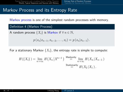
Markov process is one of the simplest random processes with memory.

Definition 4 (Markov Process)A random process {Xi} is Markov if ∀n ∈ N,

p (xn|xn−1, xn−2, . . . , x1) = p (xn|xn−1) .

For a stationary Markov {Xi}, the entropy rate is simple to compute:

H ({Xi} ) = limn→∞

H(Xn

∣∣Xn−1) Markovity

= limn→∞

H (Xn |Xn−1 )

Stationarity= H (X2 |X1 ) .




Typicality for Sources with Memory

How to extend typicality to sources with memory?

Observation:A random process with memory is characterized by joint distributionswith arbitrary length, because the depth of the memory is arbitrary.Empirical distribution π (a|xn) is insufficient to determine if thesequence is typical or not, because it only describes the marginalp.m.f. pX , not joint distributions of other lengths.

We should ask: what properties are critical for us to extend typicality tosources with memory?Recall: the most important feature of typical sequences is theAsymptotic Equipartition Property (AEP).




Xn T (n)� (X)

p�T (n)

� (X)�

� 1

|T (n)� (X)| � 2nH(X)

typical xn

p (xn) ⇡ 2�nH(X)

Suppose now we would like to give another definition of typicality andtypical set A(n)

ε . The key properties we would like to keep are:1 ∀ xn ∈ A(n)

ε , 2−n(H(X )+δ(ε)) ≤ p (xn) ≤ 2−n(H(X )−δ(ε)). (definition)

2 limn→∞

p(A(n)

ε

)= 1. (by LLN)

Why? Because the other two regarding the size of A(n)ε can be derived

from the above two properties.




Weakly Typical Sequences (for i.i.d. Random Process)

Idea: why not directly define typical sequences as those that satisfy

2−n(H(X )+δ(ε)) ≤ p (xn) ≤ 2−n(H(X )−δ(ε)) ?

Again, let p (xn) := P {Xn = xn} =∏n

i=1 pX (xi), that is, the probabilitythat the DMS generates the sequence xn.

Definition 5 (Weakly Typical Sequences for i.i.d. Random Process)For X ∼ pX and ε ∈ (0, 1), a sequence xn is called weakly ε-typical if∣∣− 1

n log p (xn)−H (X )∣∣ ≤ ε.

The weakly typical set is defined as the collection of all weakly ε-typicallength-n sequences, denoted by A(n)

ε (X).




Typical vs. Weakly Typical Sequences

Comparisons in Definition:

Typical Sequence Weakly Typical Sequence

π (·|xn) =1

n

n∑i=1

1 {xi = ·} ←→ − 1

n log p (xn) =1

n

n∑i=1

log 1

pX (xi)

pX (·) ←→ H (X )

Exercise 5Show that T (n)

ε ⊆ A(n)δ where δ = εH (X ), where in general for some ε > 0, there is

no δ′ > 0 such that A(n)δ′ ⊆ T (n)

ε .




AEP with i.i.d. Source and Weakly Typical Sequences

Proposition 2

1 ∀ xn ∈ A(n)ε (X), 2−n(H(X )+ε) ≤ p (xn) ≤ 2−n(H(X )−ε). (by definition)

2 limn→∞

p(A(n)

ε (X))= 1. (by LLN)

3 |A(n)ε (X)| ≤ 2n(H(X )+ε). (by 1 and 2)

4 |A(n)ε (X)| ≥ (1− ε)2n(H(X )−ε) for n large enough. (by 1 and 2)

Note: We only need to check that Property 2 holds, since Property 1 isautomatic by definition, and Property 3 and 4 are due to 1 and 2.This is true due to LLN: as n→∞,

− 1

n log p (xn) =1

n

n∑i=1

log 1

pX (xi)

p−→ E[log 1

pX (X)

]= H (X ) .




Stationary Ergodic Random Processes

Let’s turn to one of our original goals: finding AEP and the definition ofweakly typical sequences for random processes with memory.In other words, we would like to establish the following LLN-like keyproperty for random processes with memory: as n→∞,

− 1

n log p (xn)p−→ H ({Xi} ) .

It turns out that this is true for stationary ergodic processes.Roughly speaking, a stationary process {Xi} is ergodic if the timeaverage (empirical average) converges to the ensemble average withprobability 1. More specifically, ∀ k1, k2, . . . , km ∈ N, f measurable,

P

{lim

n→∞

1

n

n−1∑l=0

f (Xk1+l, . . . ,Xkm+l) = E [f (Xk1 , . . . ,Xkm)]

}= 1




AEP for Stationary Ergodic Processes

Theorem 3 (Shannon-McMillan-Breiman)If H ({Xi} ) is the entropy rate of a stationary ergodic process {Xi}, then

P{

limn→∞

− 1

n log p (xn) = H ({Xi} )}

= 1,

which implies that − 1n log p (xn)

p−→ H ({Xi} ) as n→∞.

With the above theorem, we can re-define weakly typical sequences as wedid in the i.i.d. case, with the following substitution: H (X )→ H ({Xi} )and derive corresponding properties. As we discussed before, the four keyproperties in Proposition 1 and 2 remain the same.




Lossless Source Coding Theorem for Ergodic DSS

Source Encoder


s[1 : N ] b[1 : K] bs[1 : N ]

Theorem 4 (A Lossless Source Coding Theorem for Ergodic DSS)For a discrete stationary ergodic source {Si}, R∗ = H ({Si} ).

Achievability can be proved as that in the DMS case, based onweakly typical sequences. The proof is identical.Converse is also the same as that in the DMS case, except that weshall make use of the following fact from Exercise 4:

1

NH(SN )

↓ H ({Si} ) as n→∞.



Summary



Lossless source coding theorem: R∗ = H, where1 H = H (S ) for DMS {Si}.2 H = H ({Si} ) for ergodic DSS {Si}.

Typical Sequence T (n)ε vs. Weakly Typical Sequence A(n)

ε

Asymptotic Equipartition Property (AEP) for both typical sequenceswith DMS and weakly typical sequences with ergodic DSS:

1 ∀ xn ∈ T (n)ε (X), 2−n(H(X )+δ(ε)) ≤ p (xn) ≤ 2−n(H(X )−δ(ε)).

∀ xn ∈ A(n)ε ({Xi}), 2−n(H({Xi} )+ε) ≤ p (xn) ≤ 2−n(H({Xi} )−ε).

2 limn→∞ p(T (n)ε (X)

)= 1. limn→∞ p

(A(n)

ε ({Xi}))= 1.

3 |T (n)ε (X)| ≤ 2n(H(X )+δ(ε)). |A(n)

ε (X)| ≤ 2n(H({Xi} )+ε).4 |T (n)

ε (X)| ≥ (1− ε)2n(H(X )−δ(ε)) for n large enough.|A(n)

ε ({Xi})| ≥ (1− ε)2n(H({Xi} )−ε) for n large enough.

Fano’s inequality


lecture 3 lossless source coding -...

Documents