lecture 21: major types of satellite imagery by austin troy university of vermont ------using gis--...

Lecture 21:Major Types of Satellite Imagery

By Austin TroyUniversity of Vermont

------Using GIS--Introduction to GIS

©2005 Austin Troy

Major satellite imagery products•SPOT

•Landsat TM

•Landsat MSS

•IKONOS

Introduction to GIS

©2005 Austin Troy

SPOT•Launched by France

• Stands for Satellite Pour l'Observation de la Terre

•Operated by the French Space Agency, Centre National d'Etudes Spatiales (CNES).

Introduction to GIS

©2005 Austin Troy

SPOT•SPOT 1 launched 1986, decommissioned and the reactivated in 1997

•SPOT 2 launched 1990, still going

•SPOT 3 launched 1993 and stopped functioning 1996

•SPOT 4 launched in 1998, still going

•SPOT 5 scheduled for April 2002

Introduction to GIS

©2005 Austin Troy

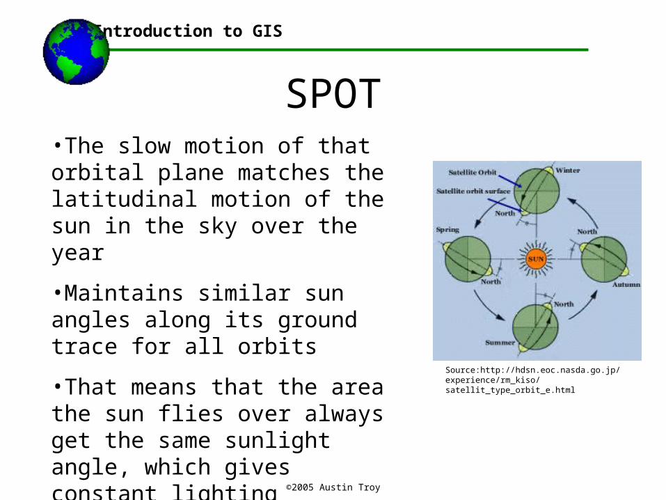
SPOT•SPOT satellites are in sun-synchronous orbit

•The satellite passes over the same part of the Earth at roughly the same local time each day

•Its “inclination” is about 8 degrees off of polar orbit

•The fact that the earth is not perfect sphere makes the orbital plane rotate slowly around the earth (this would not happen if it were perfectly polar)

Introduction to GIS

©2005 Austin Troy

SPOT•The slow motion of that orbital plane matches the latitudinal motion of the sun in the sky over the year

•Maintains similar sun angles along its ground trace for all orbits

•That means that the area the sun flies over always get the same sunlight angle, which gives constant lighting

Introduction to GIS

Source:http://hdsn.eoc.nasda.go.jp/experience/rm_kiso/satellit_type_orbit_e.html

©2005 Austin Troy

SPOT

Introduction to GIS

Source:http://ltpwww.gsfc.nasa.gov/IAS/handbook/handbook_htmls/chapter6/chapter6.html

This is for LANDSAT, but the idea is the same for SPOT

©2005 Austin Troy

SPOT•Each SPOT satellite carries two HRV (high-resolution visible) sensors, constructed with multilinear array detectors, or “pushbroom scanners”, also known as “along track scanners”

•These record multispectral image data along a wide swath

Introduction to GIS

Source: http://www.sci-ctr.edu.sg/ssc/publication/remotesense/spot.htm

©2005 Austin Troy

SPOT•Pushbroom uses a “linear array” of detectors, so it senses single column at a time, and uses forward motion to generate second dimension

•GSD (ground sampled distance), or resolution is set by sampling interval . Normally results in just-touching square pixels making up the image

•Each spectral band of sensing requires its own array.

•Pushbroom scanners generally have higher radiometric resolution because they have longer “dwell time” than across-track scanners, which move laterally across landscape as also move forward

Introduction to GIS

©2005 Austin Troy

SPOT•The position of each HRV unit can be changed by ground control to observe a region of interest that is at an oblique angle to the satellite—up to ±27º relative to the vertical.

•Off-nadir viewing allows for acquisition of stereoscopic imagery (because of the parallax created) and provides a shorter revisit interval of 1 to 3 days.

Introduction to GIS

Source: http://www.sci-ctr.edu.sg/ssc/publication/remotesense/spot.htm

©2005 Austin Troy

SPOT•Oblique viewing capacity allows it to image any area within a 900 kilometer swath; can be used to increase the viewing frequency for a given point during a given cycle. The frequency varies with latitude: at the equator, a given area can be imaged 7 times during the same 26-day orbital cycle. At latitude 45 degrees, a given area can be imaged 11 times during the orbital cycle, i.e. 157 times yearly and an average of 2.4 days, with an interval ranging from a maximum of 4 days to a minimum of 1 day.

•Any point on 95% of the earth may be imaged any day by one of the three satellites.

Introduction to GIS

Source:http://www.spot.com/home/system/introsat/acquisi/welcome.htm

©2005 Austin Troy

SPOT•Two modes: panchromatic and multispectral

•Panchromatic: single spectral band, corresponding to the visible part of the EM spectrum without the blue, from 0.51 to 0.73 µm. Single channel imaging mode, so yields black and white images. Resolution is 10 m. Pixels per line is 6000. Good for fine geometrical detail.

•Multispectral mode: three spectral bands are XS1 covering 0.50 to 0.59 µm (green), XS2 covering 0.61 to 0.68 µ m (red) and XS3 covering 0.79 to 0.89 µm (near infrared). Resolution is 20 m. Pixels per line is 3000.

Introduction to GIS

©2005 Austin Troy

SPOT•Some examples: mosaic false color tiles of Australia

Introduction to GIS

©2005 Austin Troy

SPOT

Introduction to GIS

©2005 Austin Troy

LANDSAT•first started by NASA in 1972 but later turned over to NOAA

•Since 1984 satellite operation and data handling are managed by a commercial company EOSAT

Introduction to GIS

Source: http://www.sci-ctr.edu.sg/ssc/publication/remotesense/landsat.htm

©2005 Austin Troy

LANDSAT•LANDSAT-1 launched 1972 and lasted until 1978.

•LANDSAT-2 launched 1975

•Three more satellites were launched in 1978, 1982, and 1984 (LANDSAT-3, 4, and 5 respectively).

•LANDSAT-6 was launched on October 1993 but the satellite failed to obtain orbit.

•LANDSAT-7 launched in 1999

•Only 7 and 5 are still working

Introduction to GIS

©2005 Austin Troy

LANDSAT•Like SPOT, LANDSAT is sun-synchronous, and is about 8 degrees off a polar orbit

•Its repeat cycle is about 16 days and always crosses equator at around 10 AM.

•Orbit takes about 99 minutes (14.5 per day)

•Distance between ground tracks of consecutive orbits is 2752 km at equator because of the earth’s rotation

•By following earth’s rotation with each pass, it can keep crossing the equator at the same time

Introduction to GIS

©2005 Austin Troy

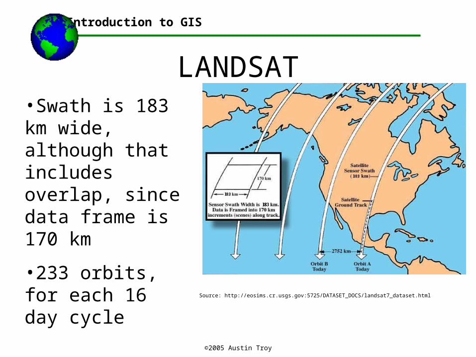
LANDSAT•Swath is 183 km wide, although that includes overlap, since data frame is 170 km

•233 orbits, for each 16 day cycle

Introduction to GIS

Source: http://eosims.cr.usgs.gov:5725/DATASET_DOCS/landsat7_dataset.html

©2005 Austin Troy

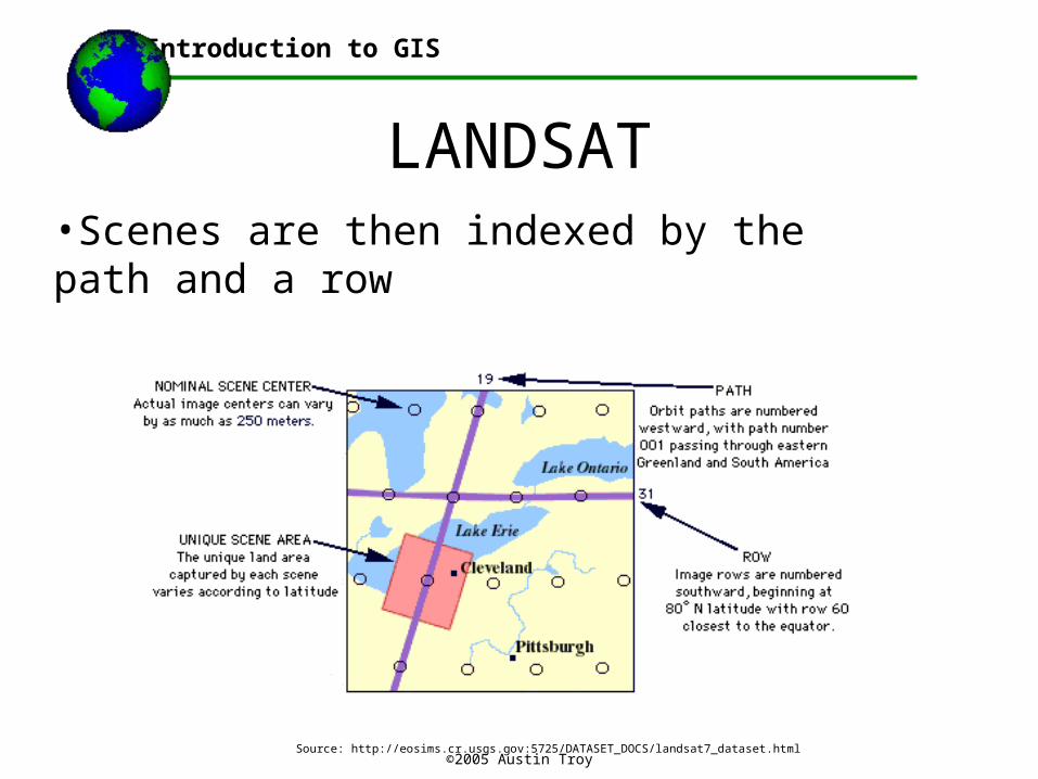
LANDSAT•Scenes are then indexed by the path and a row

Introduction to GIS

Source: http://eosims.cr.usgs.gov:5725/DATASET_DOCS/landsat7_dataset.html

©2005 Austin Troy

LANDSAT•LANDSAT 4 and 5 had two types of sensors, MSS (multi-spectral scanner) and TM (thematic mapper):

•MSS:Started on LANDSAT 1, terminated in late 1992. 80 m resolution with four spectral bands from the visible green to the near-infrared (IR) wavelengths. Only Landsat 3’s MSS sensor had a fifth band in the thermal-IR.

Introduction to GIS

©2005 Austin Troy

LANDSAT•TM: started with LANDSAT 4. Wavelength range for the TM sensor is from the visible (blue), through the mid-IR, into the thermal-IR portion of the EM spectrum. 16 detectors for the visible and mid-IR wavelength bands in the TM sensor provide 16 scan lines on each active scan. Four detectors for the thermal-IR band provide four scan lines on each active scan. The TM sensor has a spatial resolution of 30 m for the visible, near-IR, and mid-IR wavelengths and a spatial resolution of 120 m for the thermal-IR band.

Introduction to GIS

©2005 Austin Troy

LANDSAT 4 and 5MSS:

•TM:

Introduction to GIS

*

*

* Mid infra red

©2005 Austin Troy

LANDSAT MSS•MSS has a square instantaneous field of view (IFOV), with an 11.56 ° field of view.

Introduction to GIS

Source: http://edcwww.cr.usgs.gov/glis/hyper/guide/landsat

©2005 Austin Troy

LANDSAT MSS•This is a “whiskbroom” rather than “pushbroom” scanner. AKA Across track scanning

•Satellite motion provides one axis of the image and other axis provided for by oscillating mirror

•Uses four sensor arrays of six sensors each, one array for each band; six sensors are included because this allows the ground coverage rate to be achieved at one-sixth the single line scan rate.

•The analog signal is converted to digital onboard.

•Has poor radiometric resolution- only 6 bit, or 64 values

Introduction to GIS

©2005 Austin Troy

LANDSAT TM•Thematic Mapper: more bands, better spatial and radiometric resolution(256 DNs instead of 64)

•Both resolution improvements, plus the fact that the green and red bands are narrower make it better for vegetation discrimination than MSS; also near IR in TM is narrower and centered in a region that is highly sensitive to plant vigor.

Introduction to GIS

©2005 Austin Troy

LANDSAT TM•TM is also whiskbroom scanner, but collects data during both west to east and east to west sweeps of the scan mirror, unlike MSS, which only does the former

•Allows time individual detector can dwell on an area

•Scans through a field of view of 15.4°

•7 scans per second; that slow rate limits acceleration of mirror, which improves geometric integrity and boosts signal relative to noise.

•TM uses 16 detectors per band, except thermal (four)

Introduction to GIS

©2005 Austin Troy

LANDSAT TM: applications

Introduction to GIS

Band Nominal Spectral location

applications

1 Blue Water body penetration, soil-water discrimination, forest type mapping, cultural feature ID

2 Green Green reflectance peak of veg, for veg ID and assessment of vigor, cultural feature ID

3 Red Chlorophyll absorption region, plant species differentiation, cultural feature ID

4 Near infra red Veg types, vigor and biomass content, dilineating water bodies, soil moisture assessment

5 mid infra red (1.55-1.75 m)

Veg moisture, soil moisture, diff of soil from clouds

6 Thermal infra red Veg stress analysis, soil moisture, thermal mapping

7 mid infra red(2.08-2.35 m)

Discriminating mineral and rock types, veg moisture

©2005 Austin Troy

LANDSAT TM•An example:August 14, 1999 (left) and October 17, 1999 (right) images of the Salt Lake City area

• differences in color due to growing season

Introduction to GIS

©2005 Austin Troy

LANDSAT 7•Uses a new sensor called Enhanced Thematic Mapper Plus (ETM+)

•Stresses continuity with LANDSAT 4 and 5 in that uses similar orbit and repeat patterns, as well as a similar 185 km swath width for imaging

•Check out the movie

Introduction to GIS

Source: http://ltpwww.gsfc.nasa.gov/IAS/handbook/handbook_htmls/chapter2/chapter2.html

Full info at http://ltpwww.gsfc.nasa.gov/IAS/handbook/handbook_toc.html

©2005 Austin Troy

LANDSAT 7•Spatial resolution of bands

Introduction to GIS


Table 6.1 Image Dimensions for a Landsat 7 0R Product

BandNumber

Resolution(meters)

Samples(columns)

Data Lines(rows)

Bits perSample

1-5, 7 30 6,600 6000 8

6 60 3,300 3,000 8

8 15 13,200 12,000 8

©2005 Austin Troy

LANDSAT 7•Spatial resolution of bands

Introduction to GIS

LANDSAT-7 ETM+ BAND CHARACTERISTICS

Band Number

Nominal spectrum

Spectral Range (µ)

Ground Resolution

(m)

Data Lines Per Scan

Data Line Length (bytes)

1 Blue .450 to .515 30 16 6,600

2 green .525 to .605 30 16 6,600

3 red .630 to .690 30 16 6,600

4 Near IR .775 to .900 30 16 6,600

5 mid IR 1.550 to 1.750 30 16 6,600

6 Thermal IR 10.40 to 12.50 60 8 3,300

7 mid IR 2.090 to 2.35 30 16 6,600

8 panchromatic .520 to .900 15 32 13,200

Band wavelength spectrums are slightly different from LANDSAT 5

©2005 Austin Troy

LANDSAT Products•All data older than 2 years return to "public domain" and are distributed by the Earth Resource Observation System (EROS) Data Center of the US Geological Servey

•Available at http://edcwww.cr.usgs.gov/products/satellite/landsat7.html

•The LANDSAT Reference system catalogues the world into 57,784 scenes, each 115 miles (183 kilometers) wide by 106 miles (170 kilometers) long.

Introduction to GIS

©2005 Austin Troy

LANDSAT Imagery

Introduction to GIS

Composite of shortwave infrared, Near-Infrared and Red. Shows manmade features as well as densely forested areas and agricultural lands

©2005 Austin Troy

LANDSAT Imagery

Introduction to GIS

Same bands: light yellow-green color represents northern hardwood forest. The dark green patches represent various conifer species

©2005 Austin Troy

IKONOS data

Introduction to GIS

•High resolution satellite developed by Space Imaging, launched 1999

•Has sun-synchronous orbit and crosses equator at 10:30 AM

•Ground track repeats every 11 days

•Highly maneuverable: can point at a new target and stabilize itself in seconds, enabling it to follow meandering features

•The entire spacecraft moves, not just the sensors

©2005 Austin Troy

IKONOS data•Can collect data at angles of up to 45° from the along track and across track axes

•This allows for side by side and fore and aft stereoscopic imaging

•At its nadir it has 11 km swath width

•11 km by 11 km image size, but user specified strips and mosaics can be ordered

•Employs a linear array scanner

Introduction to GIS

©2005 Austin Troy

IKONOS data•IKONOS collects panchromatic band (.45 to .90 m) at 1 m resolution

•Collects four multispectral bands at 4 m resolution

•Bands include blue (.45 to .52 m) , green (.51 to .60 m) , red (.63 to .70 m), near IR (.76 to .85 m)

•Radiometric resolution is 11 bits, or 2048 values

Introduction to GIS

©2005 Austin Troy

IKONOS data•Here is 1m IKONOS view of suburbs, near winter Olympics

Introduction to GIS

Source: spaceimaging.com

lecture 21: major types of satellite imagery by austin troy university of vermont ------using gis--...

Documents

spot slide

austin troy spot introduction

gis slide

austin troy spot pushbroom

austin troy spot oblique

gis source

polar introduction

wide swath introduction