Surfing  the  Ring  

B.  Nash  27  Jan.  2015  

Outline  

•  Storage  ring  parameters  and  components  -­‐-­‐-­‐dipoles  and  orbit  

•  Linear  dynamics  

 -­‐quadrupoles  and  transverse  dynamics  

 -­‐RF  cavity  and  longitudinal  dynamics  

•  Non-­‐linear  dynamics  

•  Codes  

Storage  Ring  parameters  

gamma = 11,800 T0=2.8 microsecond

this lecture! Also: Dispersion Beta functions synchrotron tune

Dynamic aperture! “A Low-Emittance Lattice for the ESRF”, Synchrotron Radiation News, Volume 27, Issue 6, 2014

Storage  ring  components  

dipole

quadrupole

sextupole

RF cavity

Dipoles  bend  electrons  

64 dipoles, 2 per cell

2.16 m 0.29 m

B=0.85 T 92.3 mrad bend

B=0.40 T 6 mrad bend

hard bend soft bend ESRF dipoles

0.0983*64=2*pi

Closed  Orbit  from  dipoles  

How do we measure orbit?

BPM

B=.85 T p/c=6.04 GeV

ρ = 23m

Note however that for ESRF C= 844m, r=134 m This is because of straight sections: closed orbit is a 64 sided polygon

224 BPMs 7 in each cell

Bρ =Pe

B

Reference  system  

X

Y

Z

s=position along closed orbit

local coordinate system to describe electron dynamics

Global coordinates for alignment

x

y z

Phase  space  

time

phase space x vs. p

configuration space x vs. time

x=0

x

px,y = γmvx,yfor electron, we normalize with

P0 = γmvsand use

x ' = pxP0

=dxds

Phase  space  descripJon  allows  

Matrix formulation of linear optics

Hamiltonian formulation of equations of motion

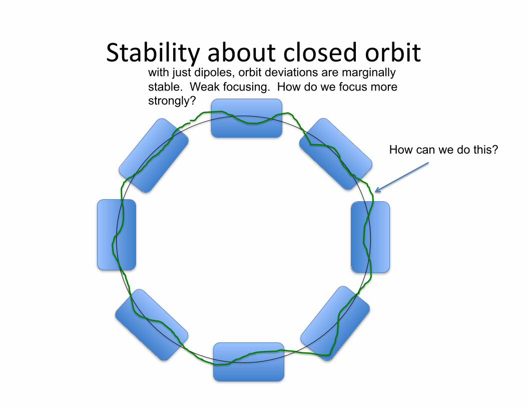
Stability  about  closed  orbit  with just dipoles, orbit deviations are marginally stable. Weak focusing. How do we focus more strongly?

How can we do this?

Quadrupoles  for  strong  focusing  of    electrons  

Bx = B1yBy = B1xBz = 0

Field in body given by

¼ of an ESRF quadrupole

∇ •!B = 0

∇ ×!B = 0

However, when we allow B1(s)We pick up Bz = B1

'xy

EquaJons  of  moJon  

x ''+ kx (s)x = 0y ''+ ky (s)y = 0

H (x, x ', y, y ') =12kxx

2 + kyy2 + x ' 2 + y' 2( )

kx = −B1Bρ

ky =B1Bρ

Can be derived from this Hamiltonian

x ' = pxP0

=dxds

Harmonic oscillator with s-dependent, periodic spring constant. Known as Hill’s equation.

kx,y (s) = kx,y (s + C)recall Bρ =Pe

!"P = e(vz ×

#B) = ev(−B1x + B1y)

divide by P0 and change time derivative to s- derivative, take v=c, and we have:

Apply Newton’s 2nd law for Lorentz force:

y ' =pyP0

=dyds

Quadrupole  focusing  

kx = −B1Bρ

ky =B1Bρ

Focusing in two planes has opposite sides!

How can we use quadrupoles so that they provide focusing in both planes?

(example of Earnshaw’s theorem- no magnetic bottles)

Simple  example  of  strong  focusing  laOce:  FODO  

F O

QF QD QF

horizontal

vertical

D O

QD QF QD

QD

QF

Matrix  Formalism  Consider a line of elements: drift spaces, dipoles, quadrupoles

1 0k 1

⎛⎝⎜

⎞⎠⎟

1 L0 1

⎛⎝⎜

⎞⎠⎟

B=0, drift length L

thin lens quad

TQF =cos kL 1

ksin kL

− k sin kL cos kL

⎛

⎝

⎜⎜⎜

⎞

⎠

⎟⎟⎟

TQD =cosh k L 1

ksinh k L

− k sinh k L cosh k L

⎛

⎝

⎜⎜⎜⎜

⎞

⎠

⎟⎟⎟⎟

k>0

k<0

xx '

⎛⎝⎜

⎞⎠⎟ 2

= a bc d

⎛⎝⎜

⎞⎠⎟

xx '

⎛⎝⎜

⎞⎠⎟ 1

thick lens quads

Matrix  formalism  can  be  generalized  to  4-­‐D  and  even  6-­‐D  

e.g. quadrupole rotated by angle theta:

TSQ = Rθ

TQF ,x 00 TQF ,y

⎛

⎝⎜⎜

⎞

⎠⎟⎟R−θ

We will find that an RF cavity can be represented with a matrix

TRF =

1 0 0 0 0 00 1 0 0 0 00 0 1 0 0 00 0 0 1 0 00 0 0 0 a b0 0 0 0 c d

⎛

⎝

⎜⎜⎜⎜⎜⎜

⎞

⎠

⎟⎟⎟⎟⎟⎟

with 6-D phase space xx 'yy 'zδ

⎛

⎝

⎜⎜⎜⎜⎜⎜⎜

⎞

⎠

⎟⎟⎟⎟⎟⎟⎟

δ =ΔEE0

Rθ =

cosθ 0 sinθ 00 1 0 0

− sinθ 0 cosθ 00 0 0 1

⎛

⎝

⎜⎜⎜⎜

⎞

⎠

⎟⎟⎟⎟

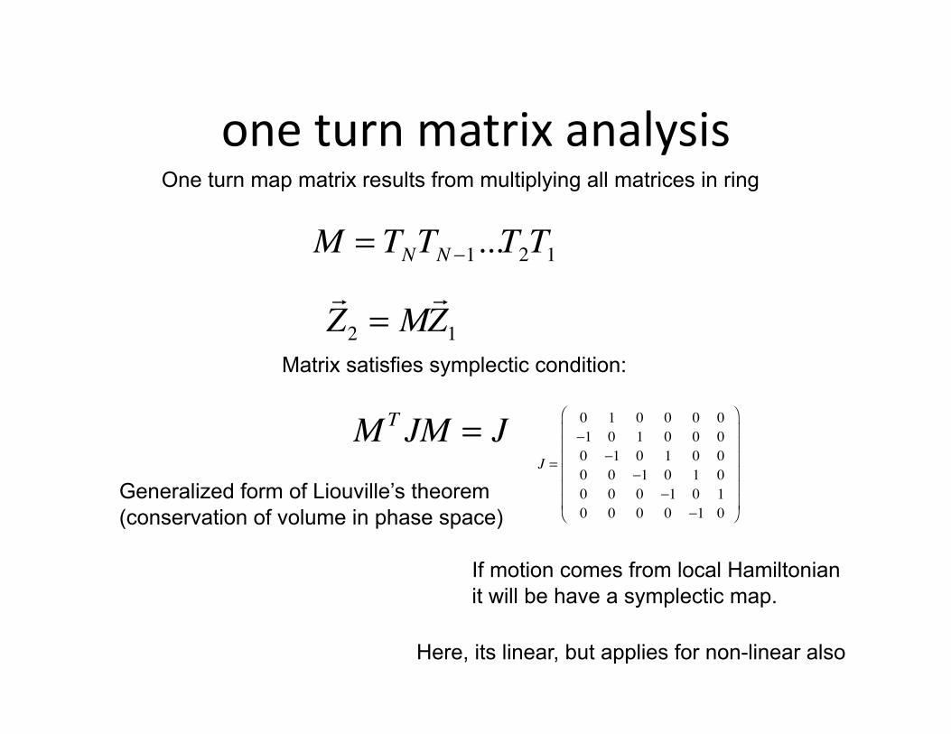
one  turn  matrix  analysis  One turn map matrix results from multiplying all matrices in ring

!Z2 = M

!Z1

Matrix satisfies symplectic condition:

MT JM = JJ =

0 1 0 0 0 0−1 0 1 0 0 00 −1 0 1 0 00 0 −1 0 1 00 0 0 −1 0 10 0 0 0 −1 0

⎛

⎝

⎜⎜⎜⎜⎜⎜

⎞

⎠

⎟⎟⎟⎟⎟⎟

Generalized form of Liouville’s theorem (conservation of volume in phase space)

If motion comes from local Hamiltonian it will be have a symplectic map.

Here, its linear, but applies for non-linear also

M = TNTN −1...T2T1

Stability  analysis  for  matrix  

µ j = 2πυ j

One can prove that eigenvalues of a symplectic matrix come in

fractional tunes! If tunes are real, then the motion is stable. If imaginary, motion is unstable.

That’s all there is to linear stability analysis!!!

λ, 1λ

pairs

λ± j = e± iµ j

or pairs of

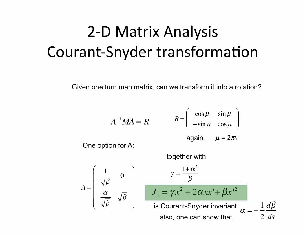
2-­‐D  Matrix  Analysis  Courant-­‐Snyder  transformaJon  

Given one turn map matrix, can we transform it into a rotation?

A−1MA = R R =cosµ sinµ− sinµ cosµ

⎛

⎝⎜

⎞

⎠⎟

One option for A:

A =

1β

0

αβ

β

⎛

⎝

⎜⎜⎜⎜⎜

⎞

⎠

⎟⎟⎟⎟⎟

Jx = γ x2 + 2αxx '+ βx '2

together with

γ =1+α 2

β

again, µ = 2πν

is Courant-Snyder invariant also, one can show that

α = −12dβds

Geometric  interpretaJon  of  Twiss  Parameters  

slope: tune is defined by number of oscillations about closed orbit over 1 turn around ring. Note that the matrix only captures fractional part.

measuring the position over time, it will oscillate

This is at one position in the ring.

invariant with position around ring!

turn 1 turn 2

turn 3

α(s)β(s)γ (s)

⎛

⎝

⎜⎜⎜

⎞

⎠

⎟⎟⎟

are known as ‘Twiss Parameters’

Transverse  dynamics  

turn 1 turn 2

turn 3

tune = phase advance per turn

position 1

position 2

position 3

Bending  with  energy  variaJon:  Dispersion  

Energy dependence of bending affects orbit: Dispersion is energy dependence of closed orbit

η ''+ k(s)η =1ρ

If no coupling, only horizontal dispersion.

ρ1ρ1 + δρbetatron oscillation with

driving term from dipoles

xCO = η(s)δ

ESRF  laOce  funcJons  

Resonances  

Integer resonance half integer

This means ν = nand map is identity

ν = n +1 / 2

Then any dipole perturbation causes an instability.

even turns

odd turns

x

x’

x

x’

Now any quadrupole perturbation causes an instability.

Eigenvalue  picture  of  linear  resonances  

integer resonance

half integer resonance

in 4-D, we have another possibility: ν x ± ν y = n

ν x + ν y = nActually only sum res. is unstable!

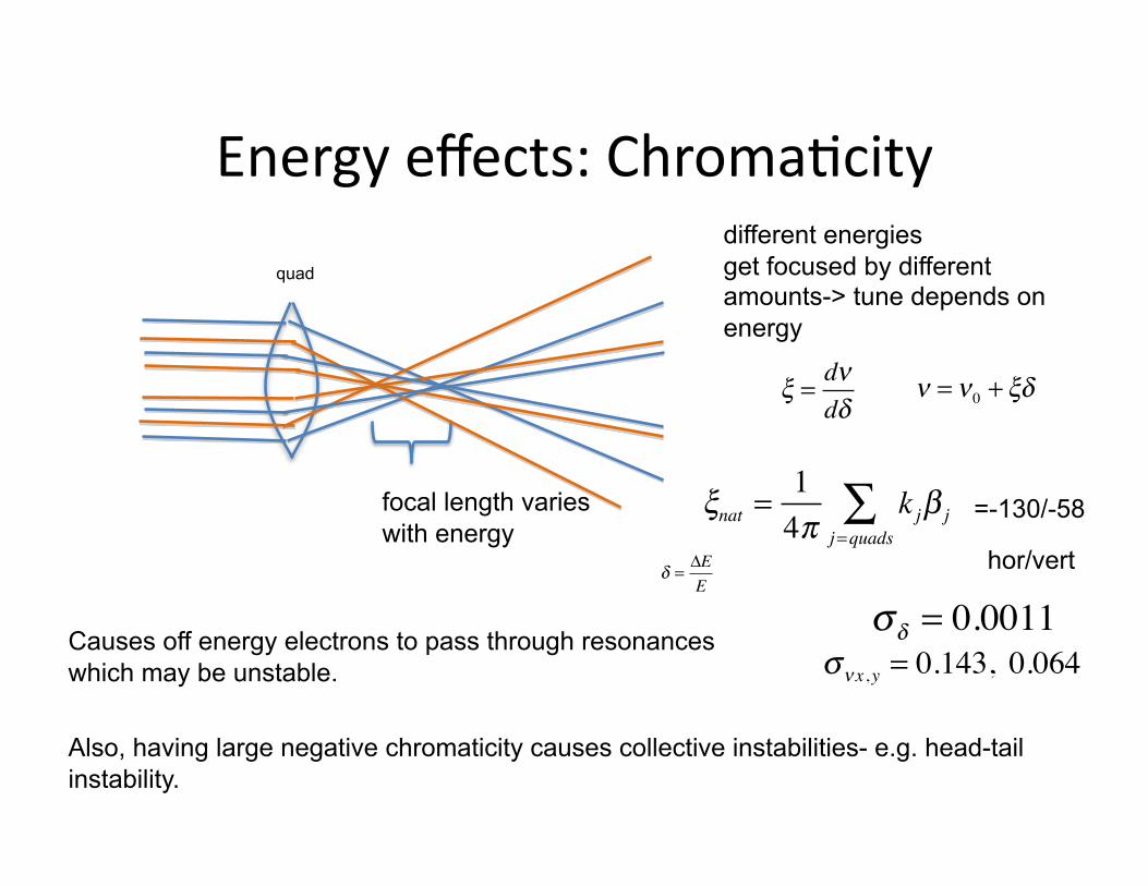
Energy  effects:  ChromaJcity  different energies get focused by different amounts-> tune depends on energy

Causes off energy electrons to pass through resonances which may be unstable.

quad

focal length varies with energy

Also, having large negative chromaticity causes collective instabilities- e.g. head-tail instability.

ξnat =14π

kjj=quads∑ β j =-130/-58

hor/vert

ξ =dνdδ

ν = ν0 + ξδ

δ =ΔEE

σδ = 0.0011σνx,y = 0.143, 0.064

Sextupoles  

Sextupoles may be used to correct chromaticity.

ChromaJcity  correcJon  with  sextupoles  

•  Dispersive  orbits  arrive  at  different  locaJons  in  sextupole  and  thus  focus  differently.  

energy dependence of focusing abberation

Bx = B2xy

By =12B2 (x

2 − y2 )

ξtot = ξnat + ξsext

ξnat =14π

kjj=quads∑ β j

ξsext =14π

η jj= sexts∑ B2 j

=-130/-58

AT ESRF, we have 7 families of sextupoles Why do we do something so complicated?

If  we  only  correct  chromaJcity…  

S. Liuzzo, PhD thesis, University of Rome, Tor Vergata (2014) Fig. 1.4

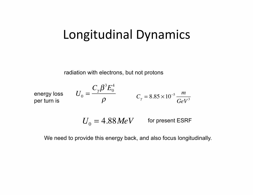
Longitudinal  Dynamics  

radiation with electrons, but not protons

We need to provide this energy back, and also focus longitudinally.

U0 =Cγ β

3E04

ρ Cγ = 8.85 ×10−5 mGeV 3

energy loss per turn is

U0 = 4.88MeV for present ESRF

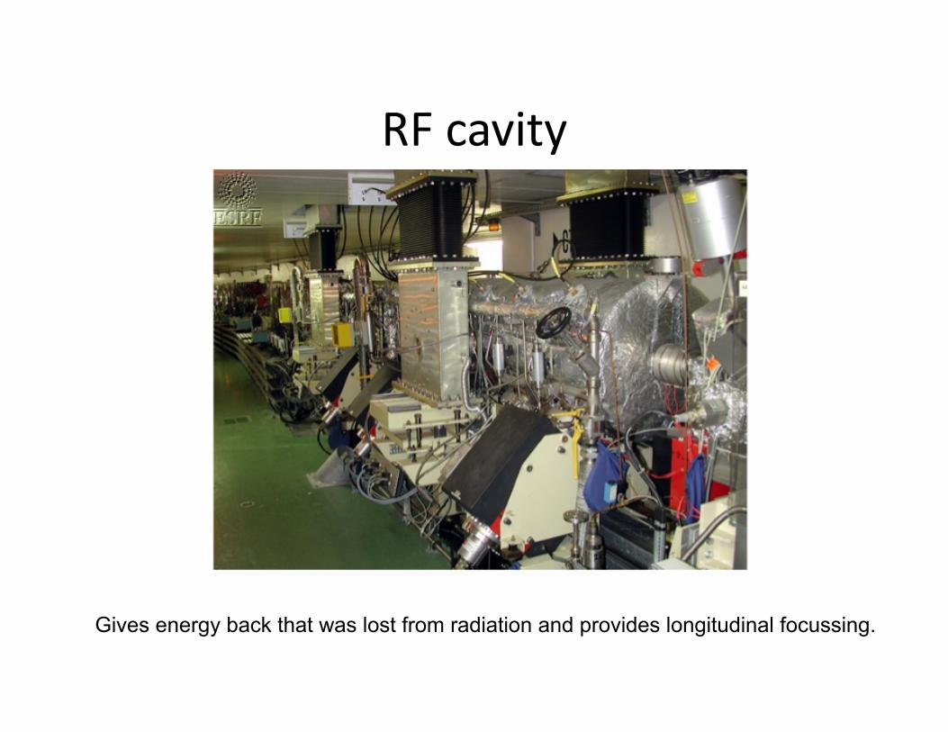
RF  cavity    

Gives energy back that was lost from radiation and provides longitudinal focussing.

RF  Buckets  

fRF=352.2 MHz h = 992

ct

dp/p RF buckets

f0=355.3KHz

harmonic number is the number of ‘RF buckets’ one can store the electrons in.

bucket 1 bucket 2 bucket 3

…

bucket 992

RF  cavity  dynamics  

V (t) = ε sin(φRF (t) + φ0 )

φRF (t) = hω0t

ΔE = eεgT sinφs = eVRF sinφsg=gap T=transit time

To energy constant, we need

ΔE =U0

energy loss from synchrotron radiation (here we assume just one

cavity)

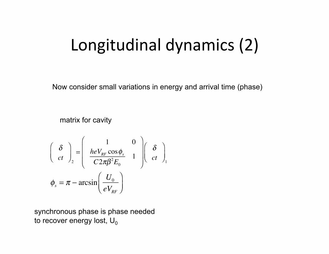
Longitudinal  dynamics  (2)  

Now consider small variations in energy and arrival time (phase)

matrix for cavity

synchronous phase is phase needed to recover energy lost, U0

φs = π − arcsin U0

eVRF

⎛⎝⎜

⎞⎠⎟

δct

⎛⎝⎜

⎞⎠⎟ 2

=1 0

heVRF cosφsC2πβ 2E0

1

⎛

⎝

⎜⎜⎜

⎞

⎠

⎟⎟⎟

δct

⎛⎝⎜

⎞⎠⎟ 1

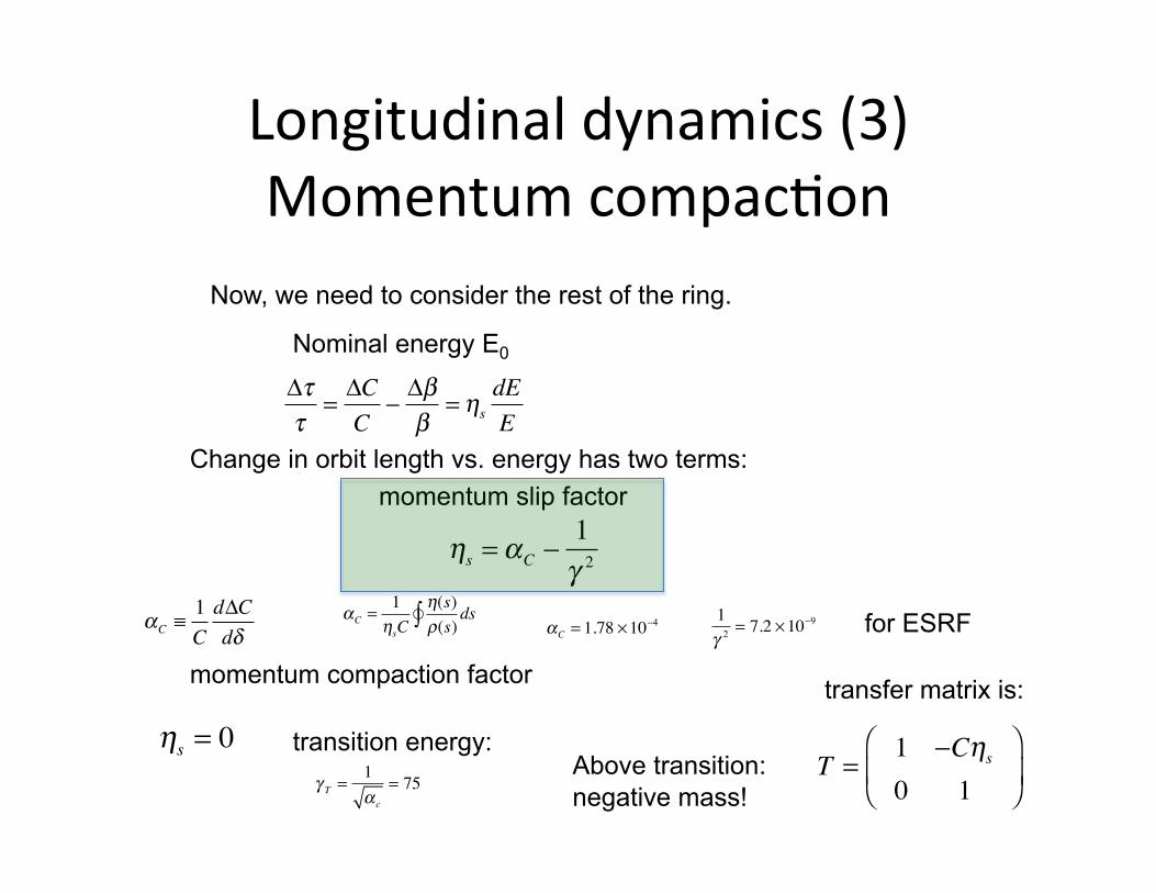
Longitudinal  dynamics  (3)  Momentum  compacJon  

Now, we need to consider the rest of the ring.

αC =

1ηsC

η(s)ρ(s)

ds!∫

T =1 −Cηs

0 1

⎛

⎝⎜

⎞

⎠⎟

momentum compaction factor

αC ≡1CdΔCdδ

ηs = αC −1γ 2

momentum slip factor

αC = 1.78 ×10−4 1γ 2 = 7.2 ×10

−9

Change in orbit length vs. energy has two terms:

for ESRF

Nominal energy E0

ηs = 0 transition energy: γ T =

1α c

= 75Above transition: negative mass!

transfer matrix is:

Δττ

=ΔCC

−Δββ

= ηsdEE

Synchrotron  tune  

ν z = 6 ×10−3

or 1 oscillation every 166 turns

δct

⎛⎝⎜

⎞⎠⎟ 2

=1 −Cηs

heVRF cosφsC2πβ 2E0

1

⎛

⎝

⎜⎜⎜

⎞

⎠

⎟⎟⎟

δct

⎛⎝⎜

⎞⎠⎟ 1

Multiplying cavity matrix with matrix for rest of ring, we find

One can now analyze this analogously as to the transverse

We derive the synchrotron tune:

µZ = 2πν z

ν z =heVRFηcosφs2πβ 2E0

and a longitudinal ‘beta function’

βz =CαC

µz

for VRF=8MV

Dynamic  Aperture  

Stored beam oscillates at small amplitudes. Linear stability analysis mainly adequate.

Not adequate for injection or beam lifetime.

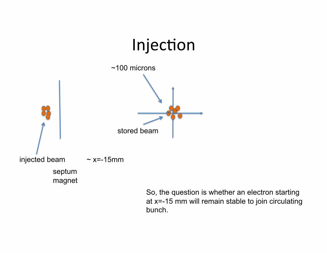
InjecJon  

stored beam

septum magnet

~ x=-15mm

~100 microns

injected beam

So, the question is whether an electron starting at x=-15 mm will remain stable to join circulating bunch.

Sextupole  non-­‐linearity  

+ =

dynamic aperture

Stable

unstable

Actually s-dependent potential.

Could add additional sextupoles and octupoles.

Dynamic  Aperture  and  frequency  map  analysis  

Frequency map by Simone Liuzzo for new lattice- S28

colors give tune diffusion related to Lyaponov exponent

Review of single particle dynamics for third generation light sources through frequency map analysis Phys. Rev. ST Accel. Beams 6, 114801 L. Nadolski, J. Laskar (2003)

2048 turns

x-y space dynamic aperture

“tune footprint” of dynamic aperture

reference

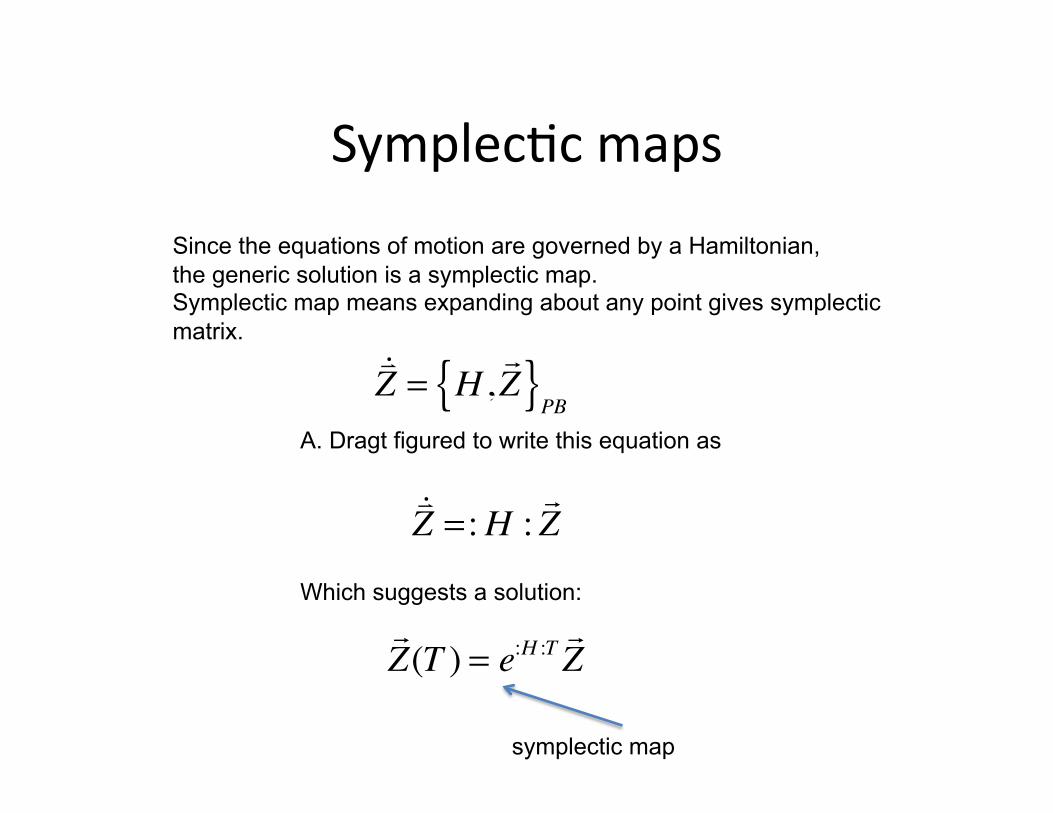
SymplecJc  maps  

Since the equations of motion are governed by a Hamiltonian, the generic solution is a symplectic map. Symplectic map means expanding about any point gives symplectic matrix.

!"Z = H ,

#Z{ }PB

A. Dragt figured to write this equation as

!"Z = :H :

#Z

Which suggests a solution:

!Z(T ) = e:H :T

!Z

symplectic map

General  SymplecJc  Maps  

Dragt and Finn proved that a general symplectic map could be written in the form

M = e:H j :

j∏

This is called Dragt-Finn factorization.

Nice, but we still don’t know how to find the dynamic aperture.

Alex Dragt, John Finn ‘Lie series and invariant functions for analytic symplectic maps J. Math. Phys. 17, 2215 (1976)

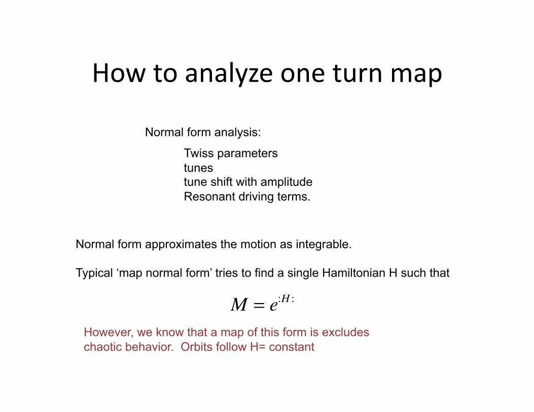
How  to  analyze  one  turn  map  

Twiss parameters tunes tune shift with amplitude Resonant driving terms.

Normal form analysis:

Normal form approximates the motion as integrable.

Typical ‘map normal form’ tries to find a single Hamiltonian H such that

M = e:H :

However, we know that a map of this form is excludes chaotic behavior. Orbits follow H= constant

Normal  Form  (2)  

E. Forest, M. Berz, J. Irwin, “Normal form methods for complicated periodic systems "A complete solution using differential algebra and lie operators." Particle Accelerators,24-91,1989

U −1MU = N where N is “as simple as possible”

General solution for arbitrary power series map

implemented in E. Forest’s LieLib Fortran90 library and used in code PTC

Given map M, find canonical transformation U, such that

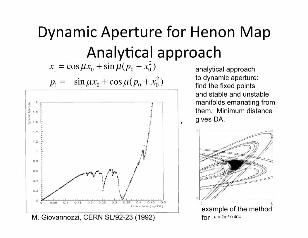
Dynamic  Aperture  for  Henon  Map  AnalyJcal  approach  

M. Giovannozzi, CERN SL/92-23 (1992)

x1 = cosµx0 + sinµ(p0 + x02 )

p1 = − sinµx0 + cosµ(p0 + x02 )

x1 = cosµx0 + sinµ(p0 + x02 )

p1 = − sinµx0 + cosµ(p0 + x02 )

analytical approach to dynamic aperture: find the fixed points and stable and unstable manifolds emanating from them. Minimum distance gives DA.

example of the method for µ = 2π *0.404

AddiJonal  effects  complicaJng  moJon  

•  damping-­‐  several  thousand  turns  (actually  helps  us  a  lot,  vs.  Hadron  machines)  

•  quantum  diffusion  (not  a  big  effect  on  DA)  

•  longitudinal  moJon  

(can  be  an  important  effect)  

SymplecJc  Integrators  •  Approximate  element  by  exactly  solvable  segments  and  

combine.    Yoshida  method  gives  a  way  to  get  an  arbitrary  order  integrator.    Typically  one  uses  4th  order.  

•  This  method  is  extended  by  Wu,  Forest  and  Robin  to  include  wigglers,  undulators  and  fringe  fields.  

•  StarJng  from  a  general  magneJc  field  representaJon  of  the  undulator,  one  uses  the  kick  map  method  of  Elleaume.  

• Construction of higher order symplectic integrators H. Yoshida, Phys. Lett. A, 150, (5-7), 262 (1990) • Y Wu, E. Forest, and D. S. Robin, “Explicit higher order symplectic integrator for s-dependent magnetic fields”, Phys. Rev. E, 68 (2003) • P. Elleaume, A New Approach to the Electron Beam Dynamics in Undulators and Wigglers

some references

Tracking  Code  Example:  Accelerator  Toolbox  

Elegant (APS, M. Borland et. al.) MadX (CERN, well organized module structure)

PTC (E. Forest, MADX interface)

developed by A. Terebilo at SLAC originally, now an ESRF version with some collaboration with other labs: atcollab http://sourceforge.net/projects/atcollab/ Other commonly used codes

Lattice is represented in Matlab in a cell array

Example of one cell:

>> S28{6}

ans =

FamName: 'QF1A' PassMethod: 'QuadMPoleFringePass' Class: 'Quadrupole' Length: 0.2950 K: 0 PolynomB: [0 2.7224] MaxOrder: 1 PolynomA: [0 0] NumIntSteps: 20 RefRadius: 0.0130 Energy: 6.0000e+09

integration routine written in C. We modify these to try to improve model, but keep speed.

ringpass(S28,[.005 0 0 0 0 0]',1000)

tracks a particle offset in x by 5 mm for 1000 turns

Scanning  sextupole  seOngs  

M. Borland et. al. ‘Multi-objective direct optimization of dynamic acceptance and lifetime for potential upgrades of the Advanced Photon Source’ ANL/APS/LS-319

N. Carmignani, PhD thesis, Univ. Pisa/ESRF (2014). Tracking code Elegant was used. Sextupole parameter space was searched using a genetic algorithm

see also for further reference

red dot is original configuration.

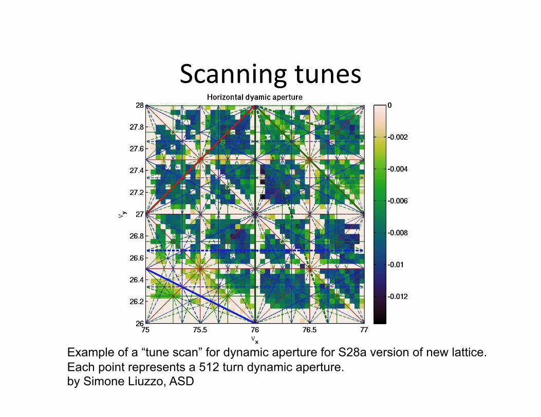
Scanning  tunes  

Example of a “tune scan” for dynamic aperture for S28a version of new lattice. Each point represents a 512 turn dynamic aperture. by Simone Liuzzo, ASD

Summary  

•  Closed  orbit  determined  by  dipoles  •  Focusing  provided  by  quadrupoles  •  Linear  stability  problem  treated  by  matrix  formulaJon  

•  Longitudinal  dynamics  treated  by  matrices  also  (synchrotron  tune)  

•  Sextupoles  needed  to  correct  chromaJcity  

•  Dynamic  aperture  opJmizaJon  sJll  a  challenging  non-­‐linear  dynamics  problem  

wave image on first slide from http://www.wallpaperbod.com/wp-content/uploads/2013/05/Sea-Water-Waves-Nature.jpg

General References

Klaus Wille, ‘The Physics of Particle Accelerators’, Oxford University Press, 1996

S.Y. Lee, ‘Accelerator Physics’, World Scientific, 1999

Helmut Wiedemann, ‘Particle Accelerator Physics’, Springer-Verlag, 1993

Next  Jme:  

•  RadiaJon  damping  and  diffusion  •  Scadering  off  of  other  electrons  and  stray  atoms  leads  to  beam  lifeJme  

•  InteracJon  with  vacuum  chamber  couples  parJcle  moJon  together  and  can  lead  to  collecJve  instabiliJes  

Thank you for your attention!!

Extra  Slides  

Hamiltonian  formulaJon  of  equaJons  of  moJon  

�

H( ! x , ! p ) = eφ + c m2c 2 + ! p − e! A c

⎛ ⎝ ⎜

⎞ ⎠ ⎟ 2

�

d! P

dt= e(! E +! v c×! B )

�

! E = −

! ∇ φ −

1c∂! A ∂t

�

! B =! ∇ ×! A

Lorentz  Force  equaJon  

(Ruth,  SLAC-­‐PUB-­‐3836)  

�

˙ x i =∂H∂pi

˙ p i = −∂H∂xi

including terms up to sextupoles:

(Bengtsson, SLS tech note, p8)

gauge  freedom  of  A  We have some freedom in choosing A. Suppose

A−1MA = R

Now, define

A = Ar for some arbitrary rotation, r

Then r−1A−1MAr = RA−1MA = rRr−1 = r

So, A−1MA = R

So A and A are equivalent canonical transformations.