lecture 2

Model PDEs PDE problem Classification Hyperbolic equations Parabolic equations Elliptic equations Numerical discretization

Lecture 2Model equations, Classification of PDEs

Introduction to Computational Fluid DynamicsThe University of New Mexico

ME 461/561

1 / 26


Outline

Model PDEs

PDE problem

Classification

Hyperbolic equations

Parabolic equations

Elliptic equations

Numerical discretizationSpectralFinite elementFinite difference and finite volume

2 / 26


Model equations

Why do we need them:

Represent essential features of full governing equations

Easier to solve numerically – can be used to develop numericalmethods

Can be solved analytically; The exact analytical solutions canbe used to verify numerical models

3 / 26


Model equations

Heat equation: ∂u∂t = a2∇2u

1D heat equation: ∂u∂t = a2 ∂2u

∂x2

Poisson (Laplace) equation: ∇2u = f (x)

2D Poisson (Laplace) equation: ∂2u∂x2 + ∂2u

∂y2 = f (x , y)

Wave equation: ∂2u∂t2 = a2∇2u

1D wave equation: ∂2u∂t2 = a2 ∂2u

∂x2

Linear convection equation: ∂u∂t + c ∂u

∂x = 0

Burgers equation: ∂u∂t + u ∂u

∂x = µ∂2u∂x2

Generic transport equation: ∂φ∂t + u ∂φ∂x = µ∂

2φ∂x2

4 / 26


Representing convection

ρ

(∂V

∂t+ (V · ∇)V

)= ρF−∇p + µ∇2V

ρC

(∂T

∂t+ V · ∇T

)= κ∇2T

Material derivative:

DΦ

Dt=∂Φ

∂t+ V · ∇Φ =

∂Φ

∂t+ u

∂Φ

∂x+ v

∂Φ

∂y+ w

∂Φ

∂z

Model analogy:

Linear convection equation:∂u

∂t+ c

∂u

∂x= 0

5 / 26


Representing diffusion

Viscous or diffusion terms in the right-hand sides:

ρ∂V

∂t+ . . . = µ∇2V

ρC∂T

∂t+ . . . = κ∇2T

Model analogy:

Heat equation:∂u

∂t= a2∇2u

If steady-state:

∇2T = f (x, t) - Poisson equation

6 / 26


Formulation of a PDE problem

A PDE problem includes:

Equation

Domain of solution

Boundary and initial conditions

Domain

Ω∂Ω

y

x

t

tend

t0

7 / 26


Types of boundary conditions

Dirichlet:u(x, t)|∂Ω = g at t0 < t < tend

Neumann:∂u(x, t)

∂n

∣∣∣∣∂Ω

= g at t0 < t < tend

Robin (mixed):(a1∂u(x, t)

∂n+ a2u(x, t)

)∣∣∣∣∂Ω

= g at t0 < t < tend

Periodic (cyclic):

u(x, t)|x0= u(x, t)|x0+L at t0 < t < tend

8 / 26


Initial conditions:

Marching problems: Time-dependent solution at t0 ≤ t ≤ tend ;Represents evolution in time. Examples: Wave, heat,linear convection, Burgers, transport

Equilibrium problems: Time-independent solution; Representssteady (equilibrium) state of the system. Examples:Laplace, Poisson

In marching problems, we need initial conditions at t = t0:

u(x, t0) = h(x) in Ω

and, in some cases,

∂u

∂t(x, t0) = f (x) in Ω

9 / 26


1D heat equation

x

u(x,t)

L

t= 0

t= ∝

T1

T2

T= T2T= T1

∂u

∂t= a2∂

2u

∂x2

Initial conditions:

u(x , t0) = u0(x) at 0 < x < L

Possible boundary conditions:

Constant end temperature – Dirichlet:u(0, t) = u0, u(L, t) = u1 at t > t0

Constant end heat flux – Neumann:∂u∂x (0, t) = u0,

∂u∂x (L, t) = u1 at t > t0

Periodic: u(0, t) = u(L, t) at t > t0

10 / 26


Poisson and Laplace equations

∇2Φ = f (x, t) or ∇2Φ = 0

Examples of possible physical situations:

Steady-state heat conduction: Φ - temperature

Steady-state acoustics: Φ - velocity potential

Incompressible fluid flows: Φ - pressure


Φ|∂Ω = g or∂Φ

∂n

∣∣∣∣∂Ω

= f

11 / 26


1D wave equation

y

x

y= u(x,t)

0L

∂2u

∂t2= a2∂

2u

∂x2

Initial conditions at t = t0:

u(x , 0) = f (x)

and

∂u

∂t(x , 0) = g(x)


u(0, t) = u1 at t > t0,

or∂u

∂x(L, t) = u2 at t > t0.

12 / 26


Mathematical classification of linear PDE of second order

Done according to existence and type of characteristics in thesolution

Different classes⇓

Different solution properties⇓

Different numerical methods

13 / 26


Characteristics

General linear equation of second order:

Aφxx + Bφxy + Cφyy + Dφx + Eφy + Fφ = G

Characteristic - a curve on the x − y plane, on whichsecond derivatives φxx, φyy, φyy are not uniquelydefined

Slope of a characteristic is:

h(x) =dy

dx=

B ±√B2 − 4AC

2A.

14 / 26


Classification

B2 − 4AC > 0 – There are two real characteristics intersecting atthis point. The equation is hyperbolic

B2 − 4AC = 0 – There is one real characteristic. The equation isparabolic

B2 − 4AC < 0 – No real characteristics exist at this point. Theequation is elliptic

15 / 26


Examples of classification

Heat equation: t → y ; A = a2, B = 0, and C = 0, soB2 − 4AC = 0 ⇒ equation is parabolic

Wave equation: t → y ; A = a2, B = 0, and C = −1, soB2 − 4AC = 4a2 ⇒ equation is hyperbolic

2D Poisson/Laplace: A = 1, B = 0, C = 1, andB2 − 4AC = −4 < 0 ⇒ equations are elliptic

16 / 26


Hyperbolic equations

Illustration: 1D wave equation ∂2u∂t2 = a2 ∂2u

∂x2

Slope of characteristics:

h =dt

dx=

0±√0 + 4a2

2a2= ±1

a

Two families of characteristics: left-running x + at = const andright-running x − at = const

D’Alembert solution:

u(x , t) = F1(x + at) + F2(x − at)

17 / 26


Wave equation: D’Alembert solution

For initial conditions u(x , 0) = f (x), ∂tu(x , 0) = g(x):

u(x , t) =f (x + at) + f (x − at)

2+

1

2a

∫ x+at

x−atg(τ)dτ.



u(x , t) =f (x + at) + f (x − at)

2+

1

2a

∫ x+at

x−atg(τ)dτ.

0

x

t

x

x−at=x

0

x+at=x

f(x)

u(x,t)

(a)

0 0

x

t

x

x−at=x

0

x+at=x

u(x,t)

(b)

0

g(x)

Oleg Zikanov (UM-Dearborn) Essential Computational Fluid Dynamics December 28, 2011 18 / 26



u(x , t) =f (x + at) + f (x − at)

2+

1

2a

∫ x+at

x−atg(τ)dτ.

0

x

t

x

x−at=x

0

x+at=x

f(x)

u(x,t)

(a)

0 0

x

t

x

x−at=x

0

x+at=x

u(x,t)

(b)

0

g(x)

Oleg Zikanov (UM-Dearborn) Essential Computational Fluid Dynamics December 28, 2011 18 / 26

18 / 26


Main property of hyperbolic systems.

Wave-like solutions: Any perturbation propagates with finite speedalong the characteristics

0

x−at=x0x+at=x0t

0t LL/a

Observer

of dependenceDomain

Domain

P

x

of influence

19 / 26


Other examples

Linear convection equation

∂u

∂t+ c

∂u

∂x= 0

Formally not hyperbolic but has wave-like solution:

u(x , t) = F (x − ct)

x = ct – right-running characteristics

Burgers equation with zero viscosity

∂u

∂t+ u

∂u

∂x= 0

Similar to linear convection, but the slope of characteristic u(x , t)is not a constant

20 / 26


Parabolic equations

Illustration: 1D heat equation ∂u∂t = a2 ∂2u

∂x2

Slope of characteristics:

h =dt

dx=

0±√0 + 0

2a2= 0

Characteristics are lines t = const

t

0tP

L

Domainof dependence

of influenceDomain

Characteristic

x(a)

0 (b)

of y

Characteristic

Pof dependence

Domain

Boundary layer

Flow

21 / 26


Elliptic equations

Illustration: 2D Laplace and Poisson equations

∂2u

∂x2+∂2u

∂y2= 0,

∂2u

∂x2+∂2u

∂y2= f (x , y)

No real characteristics

Any perturbation is felt immediately and fully in the entiredomain

22 / 26


Concept of numerical discretization

Discretization - replacement of an exact solution of aPDE problem in a continuum domain by an approximatenumerical solution in a discrete domain

Some common types of discretization:

Spectral

Finite element

Finite difference and finite volume

23 / 26


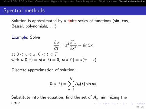
Spectral methods

Solution is approximated by a finite series of functions (sin, cos,Bessel, polynomials, . . .)

Example: Solve∂u

∂t= a2∂

2u

∂x2+ sin 5x

at 0 < x < π, 0 < t < Twith u(0, t) = u(π, t) = 0, u(x , 0) = x(π − x)

Discrete approximation of solution:

u(x , t) =N∑

n=1

An(t) sin nx

Substitute into the equation, find the set of An minimizing theerror

24 / 26


Finite element methods

Divide the solution domain into small elements (rectangular,tetrahedral, . . .)

Approximate solution in each element by a series of few (2 or3 in each direction) functions

25 / 26


Finite difference and finite volume methods

Cover the solutiondomain by a grid ofpoints

Approximate thesolution at the gridpoints

Ω∂Ω

y

x

ttend

t0

(x,y)3(x,y)1 (x,y)2

(x,y)N

(x,y)1 (x,y)2

(x,y)3(x,y)1 (x,y)2

t1

t2

tM

tM-1

t4

t3

(x,y)3

(x,y)N

(x,y)N

26 / 26

lecture 2

Documents

t ux

pde problema pde problem

t0 t tend8

t0 t tendrobin

t0 t tendneumann

vctt v t

burgers equation

t0 t tendperiodic cyclic