Lecture 22017/2018

2C/1L, MDCR Attendance at minimum 7 sessions (course + laboratory) Lectures- assistant professor Radu Damian Monday 16-18, P2 E – 50% final grade problems + (? 1 topic teory) + (2p atten. lect.) + (3 tests) +

(bonus activity)▪ 3p=+0.5p

all materials/equipments authorized Laboratory – assistant professor Radu Damian Monday 18-20 II.12 even weeks Thursday 8-14 odd weeks II.12 ? L – 25% final grade P – 25% final grade

RF-OPTO

http://rf-opto.etti.tuiasi.ro

David Pozar, “Microwave Engineering”, Wiley; 4th edition , 2011

1 exam problem Pozar

Photos

sent by email: rdamian@etti.tuiasi.ro

used at lectures/laboratory

Not customized

ADS 2016 EmPro 2015 pe baza de IP din exterior

“Engineering” Sinapses

> 2010 < 1950

Complex numbers arithmetic!!!! z = a + j · b ; j2 = -1

standard unit for angles – radians microwaves traditional unit for angles –

degrees in decimal form (55.89°)

rad 180

180

rad

0,2

,2

0,0,arctan

0,0,arctan

0,arctan

arg

anedefinit

baa

b

baa

b

aa

b

z

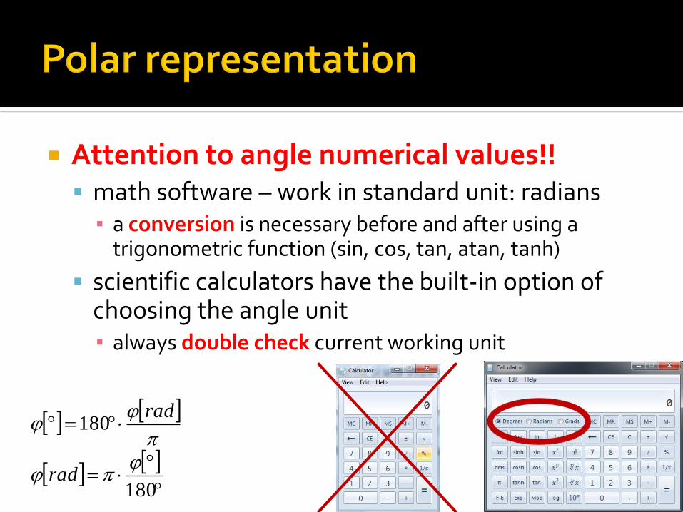
Attention to angle numerical values!! math software – work in standard unit: radians

▪ a conversion is necessary before and after using a trigonometric function (sin, cos, tan, atan, tanh)

scientific calculators have the built-in option of choosing the angle unit▪ always double check current working unit

rad 180

180

rad

0 dBm = 1 mW

3 dBm = 2 mW5 dBm = 3 mW10 dBm = 10 mW20 dBm = 100 mW

-3 dBm = 0.5 mW-10 dBm = 100 W-30 dBm = 1 W-60 dBm = 1 nW

0 dB = 1

+ 0.1 dB = 1.023 (+2.3%)+ 3 dB = 2+ 5 dB = 3+ 10 dB = 10

-3 dB = 0.5-10 dB = 0.1-20 dB = 0.01-30 dB = 0.001

dB = 10 • log10 (P2 / P1) dBm = 10 • log10 (P / 1 mW)

[dBm] + [dB] = [dBm]

[dBm/Hz] + [dB] = [dBm/Hz]

[x] + [dB] = [x]

Constitutive equationst

BE

Jt

DH

D

0 B

tJ

ED

HB

EJ

• Vacuum

mH7

0 104

mF12

0 10854,8

smc 8

00

0 1099790,21

If one of the media is a perfect conductor (metal) all fields are annulled inside

2 , 2

2 , 2

n S0

S

h

C

l n S

h

1 , 1 1 , 1

a) b)

021 EEn

SJHHn 21

SDDn 21

021 BBn

Maxwell’s Equations more simple

122 JjEE

JHH 22

Xjt

XeXX tj

0

dtetfg tj

degtf tj

E

0 H

particular cases where analytical solution exists

harmonic signals, Fourier Transform, frequency spectrum

Xjt

XeXX tj

0

dtetfg tj

degtf tj

FG

dtetfg tj

dtetfF tj

deGtg tj FG

022 EE

022 HH

j 22

γ – propagation constant (known also as phase constant or wave number)

Medium void of free electric charges

Helmoltz equations or Wave equations

Electric field only in Oy direction, through judicious choice wave traveling after Oz direction of the coordinate system

zz

y eEeEE

jj2

If we have only the positive direction wave E+=> A

zj

y eAE

Harmonic Field

ztjz

y eeAE

Amplitude

Attenuation

Wave Propagation(simultaneous space and time variation)

Wave Propagation

Circular Polarization

HjE

Lossless Medium, σ = 0

y

x

EjH

j

x

y

H

Eintrinsic impedance of the medium

ztjz

y eeAE constant phase points: const zt

Phase velocity

1

dt

dzvp

Group velocity

d

d

dt

dzvg in dispersive media where β = β(ω)

In vacuum

refractive index of a medium

3770

00

smc 8

00

0 1099790,21

0cvv g

rr

cc

0

000

11

rn

Space periodicity

f

c00

2

fT

12

Time periodicity

f

c

2

fT

12

rr f

c

00

n

cc 0

In a non-dispersive medium, εr

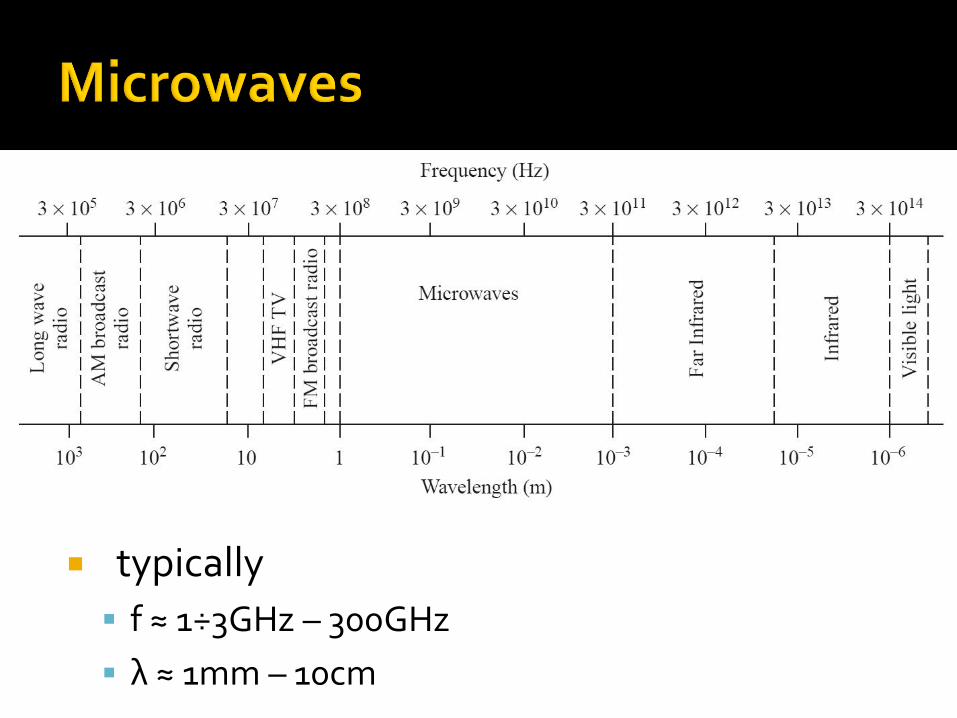
typically

f ≈ 1÷3GHz – 300GHz

λ ≈ 1mm – 10cm

Electrical Length (Phase Length) l – physical length

E = β·l – electrical Length

Dependency antenna gain

Radar cross-section

lllE 2

2

rflc

lE

0

2

V, I vary~ useless

Behavior (and description) of any circuit depends on his electrical length at the particular frequency of interest E≈0 Kirchhoff

E>0 wave propagation

lllE 2

2

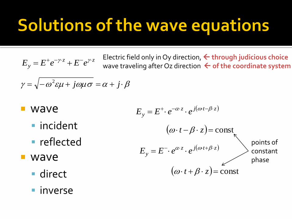
wave

incident

reflected

wave

direct

inverse

zzy eEeEE

jj2

ztjzy eeEE

ztjzy eeEE

const zt

const zt

points of constant phase

Electric field only in Oy direction, through judicious choice wave traveling after Oz direction of the coordinate system

wave

incident

reflected

wave

direct

inverse

ztjzztjzy eeEeeEE

ztjzztjzz eeHeeHH

ztjzztjz eeVeeVzV

ztjzztjz eeIeeIzI

ztjztj eVeVzV

Câmpuri electromagnetice cu variaţie armonică în timp

simplificarea ecuatiilor lui Maxwell

In medii delimitate solutiile ecuatiilor luiMaxwell trebuie sa verifice conditiile la limita

solutiile trebuie sa respecte anumite conditiisuplimentare

Xjt

XeXX tj

0

dtetfg tj

degtf tj

Campul electric trebuie sa fie perpendicular pe un peretemetalic sau nul

Campul magnetic trebuie safie tangent la un peretemetalic sau nul

2 , 2

2 , 2

n S0

S

h

C

l n S

h

1 , 1 1 , 1

a) b)

Similar cu transformata Fourier

dtetfg tj

degtf tj

1

, ii ModAEE ii ModEA ,

particular cases where analytical solution exists

harmonic signals, Fourier Transform, frequency spectrum

Xjt

XeXX tj

0

dtetfg tj

degtf tj

FG

dtetfg tj

dtetfF tj

deGtg tj FG

particular cases where analytical solution exists

wave

▪ incident

▪ reflected

wave

▪ direct

▪ inverse

zz

IN eEeEE

11

ztjzztjzy eeEeeEE

zz

OUT eEeEE

22

INE

zeE

1

zeE

1

zeE

2

zeE

2

OUTE

particular cases where analytical solution exists

modes in delimited media

1

ii ModAE ii ModEA ,

INEOUTE

N

iiOUT ModBE1

1A

NA

1B

NB

iINi ModEA ,

Source matched to load ?

Ei

Zi

ZL

I

V

impedance values ? existence of

reflections ?

Source matched to load

Ei

Ri

RL

I

V

Li

i

RR

EI

Li

Li

RR

REV

2IRP LL

22

Li

iLL

RR

ERP

Power dissipated on load Ri = 50Ω

RL = 0 PL = 0

RL = ∞ PL = 0

22

Li

iLL

RR

ERP

2IRP LL

Source matched to load

Ei

Zi

ZL

I

V

Li

i

ZZ

EI

Li

Li

ZZ

ZEV

2Re IZP LL

2

ReLi

iLL

ZZ

EZP

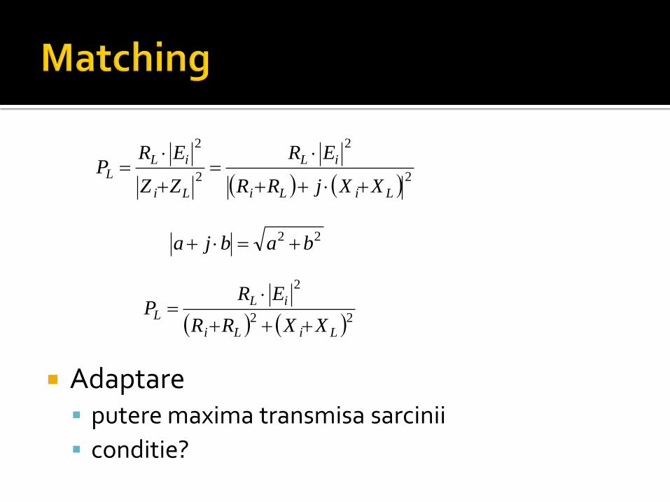
Adaptare putere maxima transmisa sarcinii

conditie?

2

2

2

2

LiLi

iL

Li

iLL

XXjRR

ER

ZZ

ERP

22 babja

22

2

LiLi

iLL

XXRR

ERP

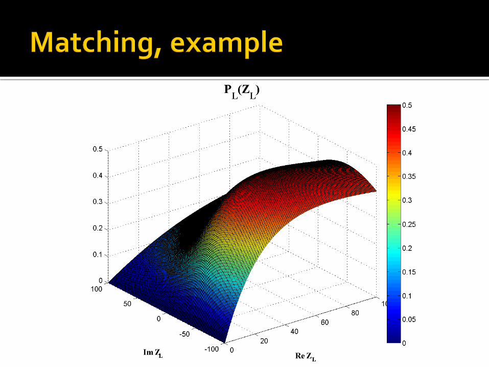
E = 10V Zi = 50 Ω +j·50Ω PL(ZL) ?

Ei

Zi

ZL

22

2

LiLi

iLL

XXRR

ERP

Pa : Available Power

L

Li

L

Lii

iL

R

XX

R

RRR

EP

22

2

4

0,0 Li RR

a

i

iL P

R

EP

4

2

max iLiL XXRR ,

*iL ZZ

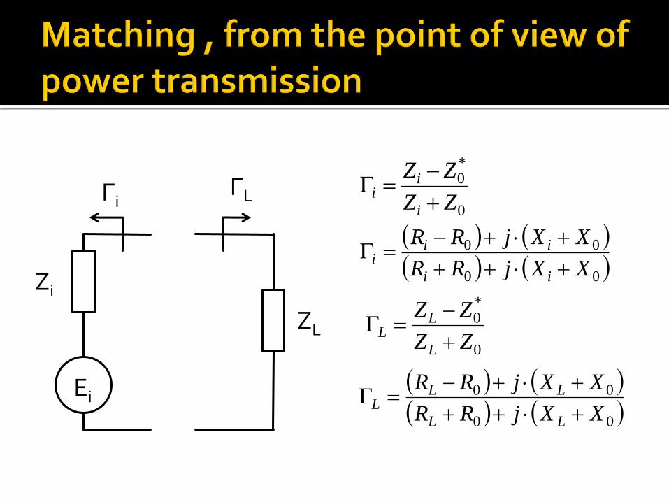
Any impedance Z0 chosen as reference

0

*0

ZZ

ZZ

Z

Γ

ZZ0

Γ

0

*0

ZZ

ZZ

i

ii

0

*0

ZZ

ZZ

L

LL

00

00

XXjRR

XXjRR

ii

iii

00

00

XXjRR

XXjRR

LL

LLL

Ei

Zi

ZL

ΓLΓi

Ei

Zi

ZL

0

*00

0

*0 1

ZZ

ZZ

ZZ

ZZ

ii

ii

ΓLΓi

0

*00

0

*0 1

ZZ

ZZ

ZZ

ZZ

LL

LL

*0

0*0

*0

*

0*0* 11

ZZ

ZZ

ZZ

ZZ

Li

i

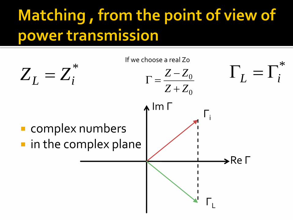
complex numbers in the complex plane

*iL ZZ

*iL

Re Γ

Im ΓΓi

ΓL

If we choose a real Z0

0

0

ZZ

ZZ

Power reflection Power of the reflected wave

Ei

Zi

ZLPa

PL

Pr

*iL ZZ

The source has the ability to sent to the load a certain maximum power (available power) Pa

For a particular load the power sent to the load is less than the maximum (mismatch) PL < Pa

The phenomenon is “as if” (model) some of the power is reflected Pr = Pa – PL

The power is a scalar !

Ei

ZiPa

aL

iL

PP

ZZ

*

Ei

Zi ZL

PL

Ei

Zi

ZL

Pa PL

Pr

+

ΓL

Zi ZL

Γi

ZiZL

Li

Lii

ZZ

ZZ

*

iL

iLL

ZZ

ZZ

*

LiLi

LiLii

XXjRR

XXjRR

iLiL

iLiLL

XXjRR

XXjRR

L

LiLi

LiLi

LiLi

LiLii

XXRR

XXRR

XXjRR

XXjRR

22

22

Li

Ei

Zi

ZLPa

PL

Pr

i

ia

R

EP

4

2

22

2

LiLi

iLL

XXRR

ERP

22

2

22

224

144

LiLi

iL

i

i

LiLi

iL

i

iLar

XXRR

RR

R

E

XXRR

ER

R

EPPP

|Γ|2 is a power reflection coefficient

2

22

222

4

a

LiLi

LiLi

i

ir P

XXRR

XXRR

R

EP

Microwave and Optoelectronics Laboratory http://rf-opto.etti.tuiasi.ro rdamian@etti.tuiasi.ro