Lecture 171

Lecture 17

Multi-Trait SelectionReference

Walsh and Lynch Ch 23, 24Xu and Muir (1992)

Lecture 172

Three Methods

• Independent Culling Levels• Tandem• Index• Combination

– Independent Culling and Index• Multi-stage Selection Index Updating • Xu and Muir (1992)

Lecture 173

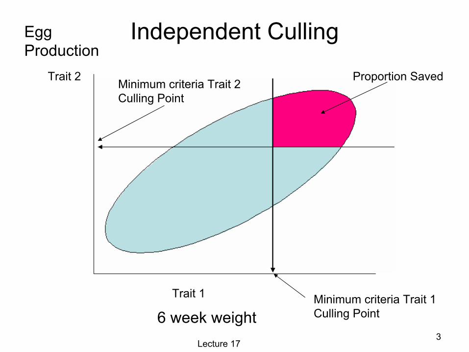
Independent Culling

Trait 1

Trait 2

Minimum criteria Trait 1Culling Point

Minimum criteria Trait 2Culling Point

Proportion Saved

6 week weight

Egg Production

Lecture 174

Tandem Culling

Trait 1

Trait 2

Minimum criteria Trait 1Culling Point

Proportion SavedGeneration 1

6 week weight

Egg Production

Lecture 175

Tandem Culling

Trait 1

Trait 2 Proportion SavedGeneration 2Minimum criteria Trait 2Culling Point

6 week weight

Egg Production

Lecture 176

Index Culling

Trait 1

Trait 2 Proportion Saved

Low Trait 2High Trait 1

Low Trait 1High Trait 2

Disadvantage in one trait off set by advantage in the other

Index line

6 week weight

Egg Production

Lecture 177

Index Updating

Trait 1

Trait 2

Index Stage 1Young Age

Proportion SavedStage 1

6 week weight

Egg Production

Lecture 178

Index Updating

Trait 1

Trait 2

Index Stage 2Later Age

Proportion Saved

6 week weight

Egg Production

Lecture 179

Theoretical Comparisons

• Same total Number of Individuals Measured – Genetic Gain

• Index Selection > Index Updating > Independent Culling > Tandem Selection

– So Why Use Anything Else But Index?• Economics• Selection Intensity

Lecture 1710

EconomicsTraits Measured At Different Life Stages

• 6 Week Weight and Egg production in Broiler Dam Lines

• Index Selection– Must Keep ALL animals until ALL traits are

Measured– Cull in one stage

• Independent Culling and Index Updating– Cull Animals As Traits Become Available– Independent Culling has NO advantages over

Index Updating

Lecture 1711

EconomicsTraits Differ Greatly in Costs to Measure

• Genotypic and Phenotypic Measures– Genotyping More Expensive than Phenotype

• Meat Quality• Measure Phenotype First• Measure Genotype on Remainder

– Phenotype More Expensive than Genotype• Annual Egg Number• Measure Genotype First• Measure Phenotype on Remainder

• Use Index Updating

Lecture 1712

Selection Intensity

• Limitations of Facilities may be different for different ages– Total Number of Individuals Measured Can be

Greater For Independent Culling or Index Updating Than Index

– Selection Intensity may be Greater for multi-stage Selection

– Depending on Selection Intensity• Index Updating > Independent Culling> Index

Selection

Lecture 1713

Example

• Limited Facilities– Index Updating or Independent

Culling• 2 Stage• Measure 10,000 chicks Stage 1• 1000 Hens Stage 2

– Index• Single Stage• Measure 1,000 chicks• Same 1000 Hens Later

• Index Selection is More Accurate• Index Updating or Independent

Culling May Have Greater Selection Intensity

Lecture 1714

Prediction of Response to Selection: Single Trait

Prediction is a process of going from a known to an unknown– Know parental values, want to

predict offspring performance– Linear Regression: Method of

Choice• Simple• Accurate within bounds• Taylor Expansion

Lecture 1715

PredictionPrior Information needed to develop calibration curve

Parental Averages

Offs

prin

g

X1

Y1

by.x

iX ,1

iY

( )mpiXYi XXbYY ,1,1.1,1 11ˆ −+= mpX ,1

1Y

X and Y same trait Measured in Different Generations

iiXYi eXbbY ,1,11,0,1 11++=

Lecture 1716

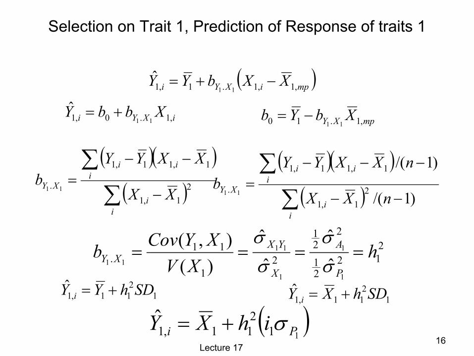
Selection on Trait 1, Prediction of Response of traits 1

( )mpiXYi XXbYY ,1,1.1,1 11ˆ −+=

( )( )( )∑

∑−

−−=

ii

iii

XYXX

XXYYb 2

1,1

1,11,1

. 11

212

21

221

21

11.

1

1

1

11

11 ˆˆ

ˆˆ

)(),( h

XVXYCovb

P

A

X

YXXY ====

σσ

σσ

1211,1 SDhXY i +=

( )11

211,1 Pi ihXY σ+=

iXYi XbbY ,1.0,1 11ˆ +=

mpXY XbYb ,1.10 11−=

1211,1 SDhYY i +=

( )( )( )∑

∑−−

−−−=

ii

iii

XYnXX

nXXYYb

)1/(

)1/(

21,1

1,11,1

. 11

Lecture 1717

In Matrix Terms: Normal Equations

=

∑∑

∑∑∑

ii

i

XYii

i

YXY

bb

XXXn

,1,1

,1

.

02,1,1

,1

11

Lecture 1718

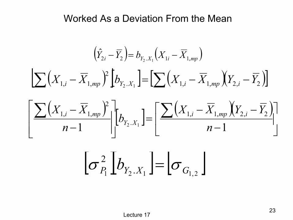
Worked As a Deviation From the Mean

( ) ( )mpiXYi XXbYY ,1,1.11 11ˆ −=−

[ ][ ] [ ]2.2

1111 GXYP b σσ =

Normal Equations

Lecture 1719

Prediction of a Second TraitPrior Information needed to develop calibration curve

Parental Averages

Offs

prin

g

Y2

iX ,1

iY2

( )mpiXYii XXbYY ,1,1.22 12ˆ −=−

mpX ,1

2Y

X and Y Different traits Measured in Different Generations

12 .XYb

1X

iiXYi eXbbY ,2,12,0,2 12++=

Lecture 1720

( )mpiXYii XXbYY ,1,1.22 12ˆ −+=

The Mean of trait 2 in the offspring can be predicted from the deviation of trait 1 in the parents

( )( )( )∑

∑−

−−=

ii

iii

XYXX

XXYYb 2

1,1

1,12,2

. 12

221

2,1

1

12.

1

2,1

12 ˆˆ

ˆˆ

)(),(

P

A

x

yxXY XV

XYCovbσ

σ

σσ

===

( )mpiP

Ai XXYY ,1,122,2

1

2,1

ˆˆˆ −+=σ

σ

1

1

2,1 ˆˆˆˆ

122,2 PP

Ai iYY σ

σ

σ+= 12,2

1

2,1

ˆˆˆ iYYP

Ai σ

σ+=

Lecture 1721

The Mean of trait 2 in the offspring can be predicted from the deviation of trait 1 in the parents

12,21

2,1

ˆˆˆ iYYP

Ai σ

σ+=

2

21

2,1 ˆˆˆ

ˆˆ12,2 P

PP

Ai iYY σ

σσ

σ+=

2

2

2

1

1

21

2,1 ˆˆˆ

ˆˆ

ˆˆˆˆ

12,2 PA

A

A

A

PP

Ai iYY σ

σσ

σσ

σσ

σ

+=

Lecture 1722

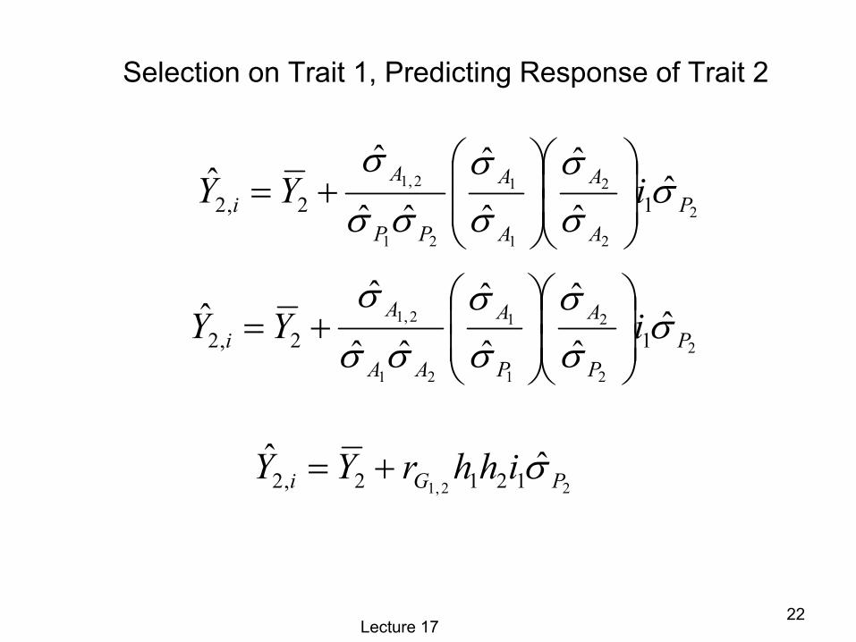
Selection on Trait 1, Predicting Response of Trait 2

2

2

2

1

1

21

2,1 ˆˆˆ

ˆˆ

ˆˆˆˆ

12,2 PA

A

A

A

PP

Ai iYY σ

σσ

σσ

σσ

σ

+=

2

2

2

1

1

21

2,1 ˆˆˆ

ˆˆ

ˆˆˆˆ

12,2 PP

A

P

A

AA

Ai iYY σ

σσ

σσ

σσ

σ

+=

22,1ˆˆ

1212,2 PGi ihhrYY σ+=

Lecture 1723

Worked As a Deviation From the Mean

( )[ ][ ] ( )( )[ ]∑∑ −−=− 2,2,1,1.2

,1,1 12YYXXbXX impiXYmpi

( ) ( )mpiXYi XXbYY ,11.22 12ˆ −=−

( ) [ ] ( )( )

−

−−=

−

− ∑∑11

2,2,1,1.

2,1,1

12 nYYXX

bnXX impi

XYmpi

[ ][ ] [ ]2,1121 .

2GXYP b σσ =

Lecture 1724

Select on Traits 1 and 2Predict Response of Trait 1

iiii eXbXbbY ,1,22.1,11.10.1,1 +++=

( ) ( ) ( ) iiii eXXbXXbYY ,12,22.11,11.11,1 +−+−=−

( ) ( )( )( )( ) ( )

( )( )( )( )

−−−−

=

−−−

−−−

∑∑

∑∑∑∑

1,12,2

1,11,1

2.1

1.12

2,22,21,1

2,21,12

1,1

YYXXYYXX

bb

XXXXXXXXXXXX

ii

ii

iii

iii

Normal Equations

Divide Both sides by n-1

=

2,1

1

22,1

2,11

2

2.1

1.12

2

A

A

PP

PP

bb

σσ

σσσσ

Lecture 1725

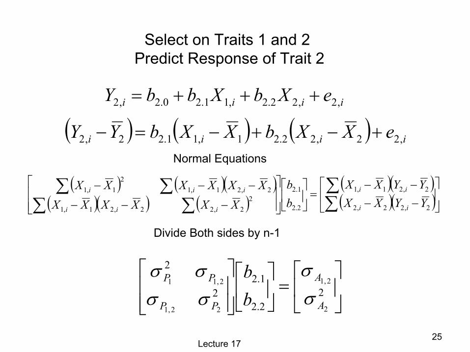
Select on Traits 1 and 2Predict Response of Trait 2

( ) ( ) ( ) iiii eXXbXXbYY ,22,22.21,11.22,2 +−+−=−

( ) ( )( )( )( ) ( )

( )( )( )( )

−−−−

=

−−−

−−−

∑∑

∑∑∑∑

2,22,2

2,21,1

2.2

1.22

2,22,21,1

2,21,12

1,1

YYXXYYXX

bb

XXXXXXXXXXXX

ii

ii

iii

iii

Normal Equations

Divide Both sides by n-1

=

2

2.2

1.22

2

2

2,1

22,1

2,11

A

A

PP

PP

bb

σσ

σσσσ

iiii eXbXbbY ,2,22.2,11.20.2,2 +++=

Lecture 1726

Select on Traits 1 and 2Predict Response of Traits 1 and 2

( ) ( )( )( )( ) ( )( )( ) ( )( )( )( ) ( )( )

−−−−−−−−

=

−−−

−−−

∑∑∑∑

∑∑∑∑

2,22,21,12,2

2,22,21,11,1

2.22.1

1.21.12

2,22,21,1

2,21,12

1,1

YYXXYYXXYYXXYYXX

bbbb

XXXXXXXXXXXX

iiii

iiii

iii

iii

Normal Equations

( ) ( ) ( ) iiii eXXbXXbYY ,12,22.11,11.11,1 +−+−=−

( ) ( ) ( ) iiii eXXbXXbYY ,22,22.21,11.22,2 +−+−=−

+

∆∆

=

∆∆

2

1

2

1

2.21.2

2.11.1

2

1

ee

XX

bbbb

YY

( ) EXBY +∆=∆

Lecture 1727

Select on Traits 1 and 2Predict Response of Traits 1 and 2

( ) ( )( )( )( ) ( )( )( ) ( )( )( )( ) ( )( )

−−−−−−−−

=

−−−

−−−

∑∑∑∑

∑∑∑∑

2,22,21,12,2

2,22,21,11,1

2.22.1

1.21.12

2,22,21,1

2,21,12

1,1

YYXXYYXXYYXXYYXX

bbbb

XXXXXXXXXXXX

iiii

iiii

iii

iii

Divide Both sides by n-1

=

2

2

2.2

1.2

2.1

1.12

2

2

2,1

2,1

1

22,1

2,11

A

A

A

A

PP

PP

bb

bb

σσ

σσ

σσσσ

GPB =

Lecture 1728

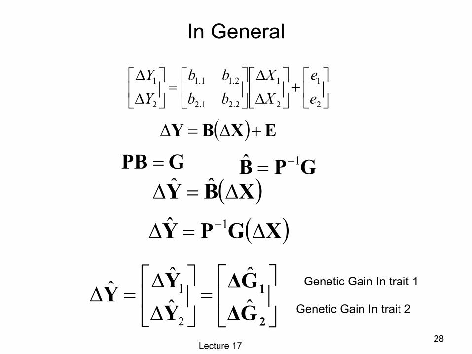
In General

GPB 1ˆ −=GPB =

+

∆∆

=

∆∆

2

1

2

1

2.21.2

2.11.1

2

1

ee

XX

bbbb

YY

( ) EXBY +∆=∆

( )XBY ∆=∆ ˆˆ

( )XGPY ∆=∆ −1ˆ

=

∆∆

=∆2

1

G∆G∆

YYY ˆ

ˆˆˆˆ2

1 Genetic Gain In trait 1

Genetic Gain In trait 2

Lecture 1729

Determining Which Traits to Select for And How Much

• Economics– Which Traits

• will produce the greatest profits?• will Respond Most Rapidly?• Are Economical to Measure?• Are some traits which are easy to measure but

with low or no economic value predictors of other more difficult or expensive to measure?

Lecture 1730

Economic Weights

Economic return that will result for each unit increase in the ith traitia

jH∆ Aggregate economic breeding value of the jth individual

∑ ∆=∆i

ijij GaH ˆ

( )XGPG ∆=∆ −1ˆ For a given individual, assume the value of the mate is the population mean, then predict the effect of selecting that individual on the offspring

Economic Breeding Value of the jth Individual

Simply Chose those individuals with the highest EBV

Lecture 1731

Breeding Program

• Method of simply choosing individuals with highest EBV’s is easy to implement but does not address the mode difficult theoretical question of which traits to measure

• Need a more theoretical predictive approach

Lecture 1732

Traits Measured and Selection Objective

• Selection Criterion – Traits Measured and selected upon

• Selection Objective– Traits Improved

• Criterion and Objective may Not be the Same– Back Fat

• Selection Criterion• easy to measure

– Feed Efficiency• Selection Objective• expensive to measure

Lecture 1733

Optimal Selection Index

mmXwXwXwZ ++= L2211

Let Z be the Selection CriterionAn index with arbitrary weights on each of m traits

pp GaGaGaQ ∆+∆+∆= L2211

Let Q be the Selection ObjectiveThe aggregate Economic Gain in p traits From Selecting

On Index Z

Problem: Find Z such that genetic gain for Q is maximum

Lecture 1734

Find Z such that genetic gain for Q is maximum

mmXwXwXwZ ++= L2211

pp GaGaGaQ ∆+∆+∆= L2211

Xw'=Z

∆Ga'=Q

Think of Z at a trait which has several sub-components

Think of Q at another trait which has several sub-components

Want to Predict Change in Q from Selection on Z

Usual Single Trait Selection Problem

Lecture 1735

Predict Change in Q from Selection on Z

∆Ga'=Q Xw'=Z

( )ZZQ ibQQ σ1.ˆ +=

Where

1)(),(ˆ i

VCovQQ

XwXw∆Ga

'

''

+=

( ) 1),(ˆ i

VCovQQ

wXwaX∆Gw

'

'

+=

1)(),(ˆ i

ZVZQCovQQ +=

Lecture 1736

),( X∆GCov Genetic Variance Covariance Matrix between all traits measured and all traits in the objective

( )XV Phenotypic Variance Covariance Matrix between all traits measured

( ) 1),(ˆ i

VCovQQ

wXwaX∆Gw

'

'

+=

G

P

PwwGaw

'

'

=

=

)(),(

ZVZQCOV

Lecture 1737

We want the regression to be maximum

1ˆ iQQ

PwwGaw'

'

+=

Maximize

PwwGaw'

'

=RLet

( ) ( ) ( )PwwGaw '' lnlnln −=R

Lecture 1738

Maximize Response in Aggregate Economic Gain

0)ln(=

wδδ R

Set

Solve for w=w

( ) ( ) ( )PwwGaw '' lnlnln 21−=R

( ) 0211)ln(21 =

−

= Pw

Pww'Ga

Gaw'wδδ R

PwGa k=

GaPw 1−= Optimal Weights

Lecture 1739

Predicting Genetic Gain in Each Trait

( )XGPG ∆=∆ −1ˆ

For any arbitrary set of weights w (including optimal)

mmXwXwXwZ ++= L2211

Xw'=Z

ZiPwwGwG'

'

=∆ ˆ

Lecture 1740

Choice of Traits

Now You can play around with different traits in the index and examine theoretical impacts

Lecture 1741

Example Broilers

Note Hi Cost to Measure Feed Efficiency and Egg Production

Lecture 1742

Economic Weights

Lecture 1743

Genetic Parameters

Lecture 1744

Optimal Index Weight and Eggs

15.75.10.65.15.10.10.09.35.6

6

RRPRwt

RRPRwt−−

23

22

21

3,23,1

3,22,1

3,12,16

6

hrrRRrhrPRrrhwtRRPRwt

PP

GP

GG

−−

−−=

6.481.144.581.146.93.234.583.236958

G

=

6.481088.253108648.1128.2538.11219881

P

=

5.5.022.

a

Lecture 1745

Optimal Weights

GaPw 1−=

Traits measured = wt6 and PR

Find optimal weights on the two traits for total economic gain and gain in each trait

−

−−= 1.146.93.23

4.583.236958G

= 648.112

8.11219881P

RR missing value but can predict

1ˆ iQQ

PwwGaw'

'

=−Optimal Weights

Genetic Gain in Economic Value

ZiPwwGwG'

'

=∆ ˆ

Genetic Gain in each trait

Lecture 1746

SAS PROGRAM

proc iml;start main;

P={19881 112.8 ,112.8 64 };

G={6958 -23.3 -58.4,-23.3 9.6 14.1};

a={.022,.5,.5};

w=inv(P)*G*a;cov=w`*G*a;VZ=w`*p*w;SZ=sqrt(vz);DH=cov*inv(SZ);DG=w`*G*inv(SZ);print w DH DG;finish main;run;quit;

Lecture 1747

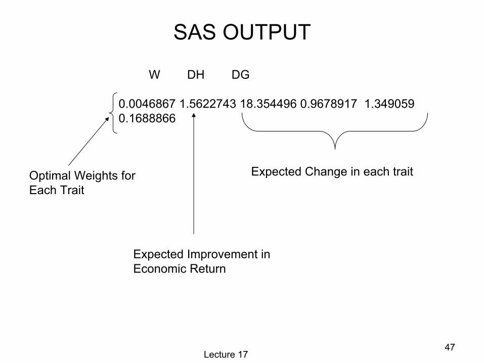
SAS OUTPUT

W DH DG

0.0046867 1.5622743 18.354496 0.9678917 1.3490590.1688866

Optimal Weights forEach Trait

Expected Improvement in Economic Return

Expected Change in each trait

Lecture 1748

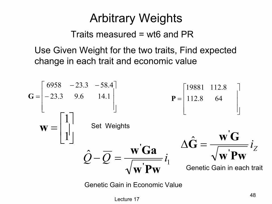
Arbitrary Weights

=11

w

Traits measured = wt6 and PR

Use Given Weight for the two traits, Find expected change in each trait and economic value

−

−−= 1.146.93.23

4.583.236958G

= 648.112

8.11219881P

1ˆ iQQ

PwwGaw'

'

=−

Set Weights

Genetic Gain in Economic Value

ZiPwwGwG'

'

=∆ ˆ

Genetic Gain in each trait

Lecture 1749

SAS PROGRAMproc iml;start main;

P={19881 112.8 ,112.8 64 };

G={6958 -23.3 -58.4,-23.3 9.6 14.1};

a={.022,.5,.5};

W={1,1};

cov=w`*G*a;VZ=w`*p*w;SZ=sqrt(vz);DH=cov*inv(SZ);DG=w`*G*inv(SZ);print w DH DG;finish main;run;quit;

Lecture 1750

SAS Output

W DH DG

1 0.8700224 48.827925 -0.096463 -0.3119211

Note Change in Economic Value Much Less than Optimal

Expected Change in each traitSet Weights forEach Trait

Lecture 1751

Lab Problem 1

• If one measure Wt6, VLDL(fat), and PR– A. What are the optimal weights– B. What is the expected change in aggregate

economic gain considering all traits of economic importance

• If one measured all traits except RR– A. What are the optimal Weight– B. What is the expected change in aggregate

economic gain considering all traits of economic importance

• Considering the costs of both programs which one do you think would be more profitable?

Lecture 1752

******************************************************* INDUPDAT ** Selection Index Updating for Maximum ** Economic Return Using the EM Type Algorithm ** By * * Shizhong Xu ** Rutgers University ** July 4, 1992 *******************************************************;OPTION LINESIZE=79;PROC IML;* P IS AN NXN PHENOTYPIC VARIANCE-COVARIANCE MATRIX;P={10816.000 13344.240 148.928 -.593 66.56,13344.240 19881 252.39 -.932 112.8,148.928 252.39 12.816 .010 4.296,-.593 -.932 .010 .003 0,66.56 112.8 4.296 0 64};* G IS AN NXK GENETIC COVARIANCE MATRIX;G={3244.8 4133.961 50.982 -.459 166.787 -8.825 -27.798,4133.961 6958.35 89.59 -.726 220.981 -23.261 -58.153,50.982 89.59 3.204 -.014 -1.622 .555 1.248,-.459 -.726 -.014 .002 .155 0 0,-8.825 -23.261 .555 0 -2.16 9.6 14.04};* W IS A KX1 VECTOR OF ECONOMIC WEIGHTS;W={0, .0011, .0148, 0, 0, .5, .5};* TOTAL PROPORTION SELECTED ;PT=1/15;* N IS AN 1XM VECTOR OF NUMBER OF TRAITS WITHIN STAGES;N={2 2 1};*N={5};* MAXIMIZE GAIN OR RATIO OR PROFIT?;MAX='PROFIT';* VCOST IS AN NX1 VECTOR OF COST PER TRAIT;VCOST={.15, .150 ,.57, 1.15,5.4};KAPA=50;BETA=1;

*PROGRAM STARTS;

m=ncol(n);c=n`;ii=n[1]; c[1]=sum(vcost[1:ii]);do jj=2 to m;ii=ii+n[jj];c[jj]=sum(vcost[ii-n[jj]+1:ii]);end;PI=3.1415926;X=PROBIT(1-PT); T=EXP(-X*X/2)/SQRT(2*PI);I=T/PT;PRINT 'VARIANCE COVARIANCE MATRICES AND ECONOMIC WEIGHTS';PRINT P; PRINT G; PRINT W c;PRINT 'TOTAL PROPORTION AND SELECTION INTENSITY';PRINT PT I;B=P**-1*G*W;DG=G`*B*I/SQRT(B`*P*B); DH=W`*DG;PRINT 'ONE STAGE INDEX SELECTION';E=PT*BETA*KAPA;COST=C[+];PROFIT=E*DH-COST;RATIO=DH/COST;START MOD;IF MAX='RATIO' THEN GOTO R;IF MAX='PROFIT' THEN GOTO P;PRINT B DG DH;GOTO G;R:PRINT B DG DH COST RATIO;GOTO G;P:PRINT B DG DH COST PROFIT;

G:I1=I;B=P[1:N[1],1:N[1]]**-1*G[1:N[1],]*W; I=N[1];DO J=2 TO M;I=I+N[J] ;QII=P[1:I,1:I]; QIJ=P[1:I-N[J],1:I]; AI=G[1:I,];BI=(I(I)-QII**-1*QIJ`*B*(B`*QIJ*QII**-1*QIJ`*B)**-1*B`*QIJ)

*QII**-1*AI*W;B=(B//J(N[J],J-1,0))||BI;END; VI=B`*P*B;B=B*SQRT(DIAG(VI))**-1;A=W`*G`*B;PRINT 'MULTI-STAGE SELECTION';PRINT B;

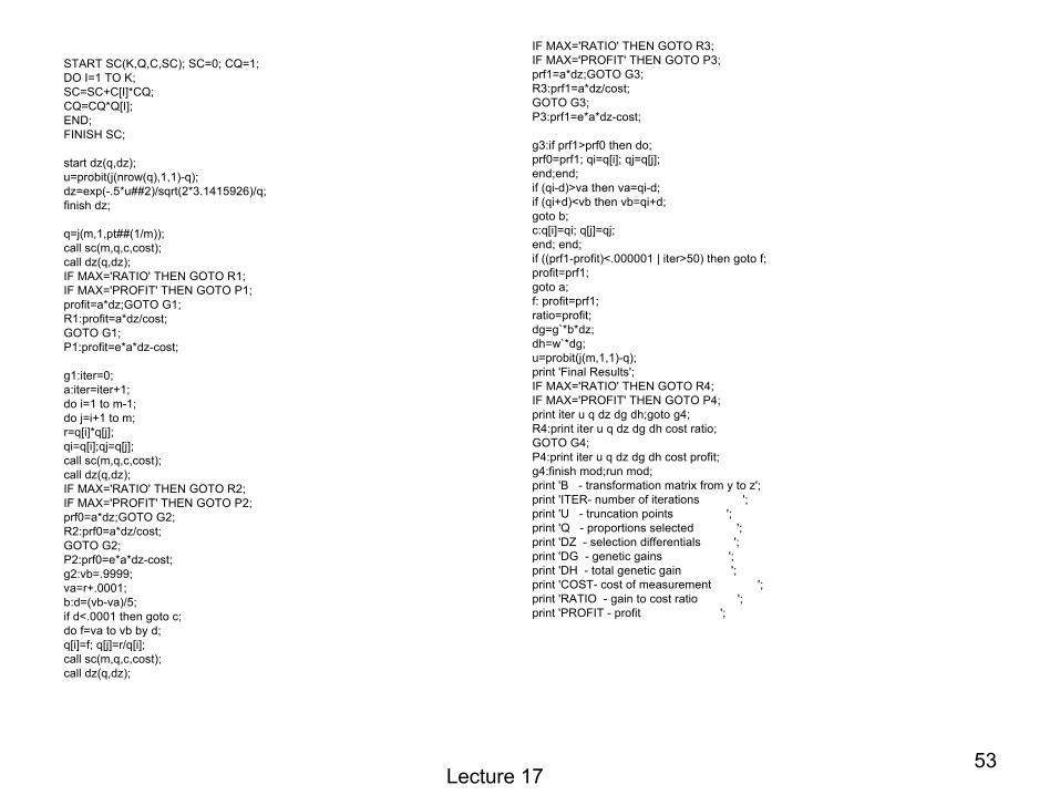
Lecture 1753

START SC(K,Q,C,SC); SC=0; CQ=1;DO I=1 TO K;SC=SC+C[I]*CQ;CQ=CQ*Q[I];END;FINISH SC;

start dz(q,dz);u=probit(j(nrow(q),1,1)-q);dz=exp(-.5*u##2)/sqrt(2*3.1415926)/q;finish dz;

q=j(m,1,pt##(1/m));call sc(m,q,c,cost);call dz(q,dz);IF MAX='RATIO' THEN GOTO R1;IF MAX='PROFIT' THEN GOTO P1;profit=a*dz;GOTO G1;R1:profit=a*dz/cost;GOTO G1;P1:profit=e*a*dz-cost;

g1:iter=0;a:iter=iter+1;do i=1 to m-1;do j=i+1 to m;r=q[i]*q[j];qi=q[i];qj=q[j];call sc(m,q,c,cost);call dz(q,dz);IF MAX='RATIO' THEN GOTO R2;IF MAX='PROFIT' THEN GOTO P2;prf0=a*dz;GOTO G2;R2:prf0=a*dz/cost;GOTO G2;P2:prf0=e*a*dz-cost;g2:vb=.9999;va=r+.0001;b:d=(vb-va)/5;if d<.0001 then goto c;do f=va to vb by d;q[i]=f; q[j]=r/q[i];call sc(m,q,c,cost);call dz(q,dz);

IF MAX='RATIO' THEN GOTO R3;IF MAX='PROFIT' THEN GOTO P3;prf1=a*dz;GOTO G3;R3:prf1=a*dz/cost;GOTO G3;P3:prf1=e*a*dz-cost;

g3:if prf1>prf0 then do;prf0=prf1; qi=q[i]; qj=q[j];end;end;if (qi-d)>va then va=qi-d;if (qi+d)<vb then vb=qi+d;goto b;c:q[i]=qi; q[j]=qj;end; end;if ((prf1-profit)<.000001 | iter>50) then goto f;profit=prf1;goto a;f: profit=prf1;ratio=profit;dg=g`*b*dz;dh=w`*dg;u=probit(j(m,1,1)-q);print 'Final Results';IF MAX='RATIO' THEN GOTO R4;IF MAX='PROFIT' THEN GOTO P4;print iter u q dz dg dh;goto g4;R4:print iter u q dz dg dh cost ratio;GOTO G4;P4:print iter u q dz dg dh cost profit;g4:finish mod;run mod;print 'B - transformation matrix from y to z';print 'ITER- number of iterations ';print 'U - truncation points ';print 'Q - proportions selected ';print 'DZ - selection differentials ';print 'DG - genetic gains ';print 'DH - total genetic gain ';print 'COST- cost of measurement ';print 'RATIO - gain to cost ratio ';print 'PROFIT - profit ';

Lecture 1754

Index Updating

ONE STAGE INDEX SELECTION

B DG DH COST PROFIT0.0066673 -11.11706 3.063772 7.42 2.7925732-0.008675 -31.080970.1146971 0.0764045-2.094819 -0.003140.1850733 -2.1065552.4353458

Lecture 1755

MULTI-STAGE SELECTION

MULTI-STAGE SELECTIONB

0.0150606 0.0036846 0.0002105-0.015502 -0.006832 -0.000383

0 0.3278797 -0.0373480 -4.189784 0.04724020 0 0.12649

DG DH COST PROFIT

-16.81431 2.4499631 2.4854298 5.6811138-50.37834-0.182759-0.001648-2.5147021.91988493.0962833

Lecture 1756

Lab Problem 2

• Examine Alternative Multi-Stage selection programs to optimize profits