lecture 15 - the university of manchestersf/20912lecture15.pdflecture 15 sergei fedotov ......
TRANSCRIPT
Lecture 15
Sergei Fedotov
20912 - Introduction to Financial Mathematics
Sergei Fedotov (University of Manchester) 20912 2010 1 / 6
Lecture 15
1 Black-Scholes Equation and Replicating Portfolio
2 Static and Dynamic Risk-Free Portfolio
Sergei Fedotov (University of Manchester) 20912 2010 2 / 6
Replicating Portfolio
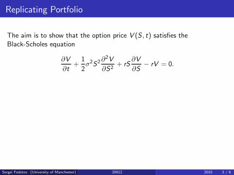
The aim is to show that the option price V (S , t) satisfies theBlack-Scholes equation
∂V
∂t+
1
2σ2
S2 ∂2V
∂S2+ rS
∂V
∂S− rV = 0.
Sergei Fedotov (University of Manchester) 20912 2010 3 / 6

Replicating Portfolio
The aim is to show that the option price V (S , t) satisfies theBlack-Scholes equation
∂V
∂t+
1
2σ2
S2 ∂2V
∂S2+ rS
∂V
∂S− rV = 0.
Consider replicating portfolio of ∆ shares held long and N bonds heldshort.
Sergei Fedotov (University of Manchester) 20912 2010 3 / 6

Replicating Portfolio
The aim is to show that the option price V (S , t) satisfies theBlack-Scholes equation
∂V
∂t+
1
2σ2
S2 ∂2V
∂S2+ rS
∂V
∂S− rV = 0.
Consider replicating portfolio of ∆ shares held long and N bonds heldshort. The value of portfolio: Π = ∆S − NB . Recall that a pair (∆,N) iscalled a trading strategy.
How to find (∆,N) such that Πt = Vt?
• SDE for a stock price S(t) : dS = µSdt + σSdW .
• Equation for a bond price B (t) : dB = rBdt.
Sergei Fedotov (University of Manchester) 20912 2010 3 / 6
Derivation of the Black-Scholes Equation
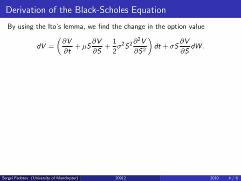
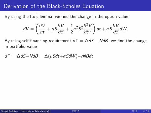
By using the Ito’s lemma, we find the change in the option value
dV =
(
∂V
∂t+ µS
∂V
∂S+
1
2σ2
S2 ∂2V
∂S2
)
dt + σS∂V
∂SdW .
Sergei Fedotov (University of Manchester) 20912 2010 4 / 6
Derivation of the Black-Scholes Equation
By using the Ito’s lemma, we find the change in the option value
dV =
(
∂V
∂t+ µS
∂V
∂S+
1
2σ2
S2 ∂2V
∂S2
)
dt + σS∂V
∂SdW .
By using self-financing requirement dΠ = ∆dS −NdB , we find the changein portfolio value
dΠ = ∆dS−NdB = ∆(µSdt+σSdW )−rNBdt
Sergei Fedotov (University of Manchester) 20912 2010 4 / 6

Derivation of the Black-Scholes Equation
By using the Ito’s lemma, we find the change in the option value
dV =
(
∂V
∂t+ µS
∂V
∂S+
1
2σ2
S2 ∂2V
∂S2
)
dt + σS∂V
∂SdW .
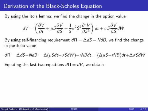
By using self-financing requirement dΠ = ∆dS −NdB , we find the changein portfolio value
dΠ = ∆dS−NdB = ∆(µSdt+σSdW )−rNBdt = (∆µS−rNB)dt+∆σSdW
Sergei Fedotov (University of Manchester) 20912 2010 4 / 6
Derivation of the Black-Scholes Equation
By using the Ito’s lemma, we find the change in the option value
dV =
(
∂V
∂t+ µS
∂V
∂S+
1
2σ2
S2 ∂2V
∂S2
)
dt + σS∂V
∂SdW .
By using self-financing requirement dΠ = ∆dS −NdB , we find the changein portfolio value
dΠ = ∆dS−NdB = ∆(µSdt+σSdW )−rNBdt = (∆µS−rNB)dt+∆σSdW
Equating the last two equations dΠ = dV , we obtain
Sergei Fedotov (University of Manchester) 20912 2010 4 / 6

Derivation of the Black-Scholes Equation
By using the Ito’s lemma, we find the change in the option value
dV =
(
∂V
∂t+ µS
∂V
∂S+
1
2σ2
S2 ∂2V
∂S2
)
dt + σS∂V
∂SdW .
By using self-financing requirement dΠ = ∆dS −NdB , we find the changein portfolio value
dΠ = ∆dS−NdB = ∆(µSdt+σSdW )−rNBdt = (∆µS−rNB)dt+∆σSdW
Equating the last two equations dΠ = dV , we obtain
∆ = ∂V
∂S,
Sergei Fedotov (University of Manchester) 20912 2010 4 / 6

Derivation of the Black-Scholes Equation
By using the Ito’s lemma, we find the change in the option value
dV =
(
∂V
∂t+ µS
∂V
∂S+
1
2σ2
S2 ∂2V
∂S2
)
dt + σS∂V
∂SdW .
By using self-financing requirement dΠ = ∆dS −NdB , we find the changein portfolio value
dΠ = ∆dS−NdB = ∆(µSdt+σSdW )−rNBdt = (∆µS−rNB)dt+∆σSdW
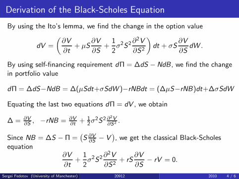
Equating the last two equations dΠ = dV , we obtain
∆ = ∂V
∂S, −rNB = ∂V
∂t+ 1
2σ2S2 ∂2V
∂S2 .
Sergei Fedotov (University of Manchester) 20912 2010 4 / 6
Derivation of the Black-Scholes Equation
By using the Ito’s lemma, we find the change in the option value
dV =
(
∂V
∂t+ µS
∂V
∂S+
1
2σ2
S2 ∂2V
∂S2
)
dt + σS∂V
∂SdW .
By using self-financing requirement dΠ = ∆dS −NdB , we find the changein portfolio value
dΠ = ∆dS−NdB = ∆(µSdt+σSdW )−rNBdt = (∆µS−rNB)dt+∆σSdW
Equating the last two equations dΠ = dV , we obtain
∆ = ∂V
∂S, −rNB = ∂V
∂t+ 1
2σ2S2 ∂2V
∂S2 .
Since NB = ∆S − Π =(
S∂V
∂S− V
)
, we get the classical Black-Scholesequation
∂V
∂t+
1
2σ2
S2 ∂2V
∂S2+ rS
∂V
∂S− rV = 0.
Sergei Fedotov (University of Manchester) 20912 2010 4 / 6
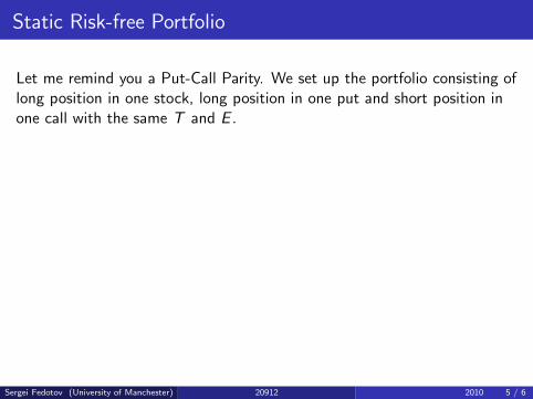
Static Risk-free Portfolio
Let me remind you a Put-Call Parity. We set up the portfolio consisting oflong position in one stock, long position in one put and short position inone call with the same T and E .
Sergei Fedotov (University of Manchester) 20912 2010 5 / 6

Static Risk-free Portfolio
Let me remind you a Put-Call Parity. We set up the portfolio consisting oflong position in one stock, long position in one put and short position inone call with the same T and E . The value of this portfolio isΠ = S + P − C .
Sergei Fedotov (University of Manchester) 20912 2010 5 / 6
Static Risk-free Portfolio
Let me remind you a Put-Call Parity. We set up the portfolio consisting oflong position in one stock, long position in one put and short position inone call with the same T and E . The value of this portfolio isΠ = S + P − C .The payoff for this portfolio is
ΠT = S + max (E − S , 0) − max (S − E , 0)
Sergei Fedotov (University of Manchester) 20912 2010 5 / 6
Static Risk-free Portfolio
Let me remind you a Put-Call Parity. We set up the portfolio consisting oflong position in one stock, long position in one put and short position inone call with the same T and E . The value of this portfolio isΠ = S + P − C .The payoff for this portfolio is
ΠT = S + max (E − S , 0) − max (S − E , 0) = E
The payoff is always the same whatever the stock price is at t = T .
Sergei Fedotov (University of Manchester) 20912 2010 5 / 6

Static Risk-free Portfolio
Let me remind you a Put-Call Parity. We set up the portfolio consisting oflong position in one stock, long position in one put and short position inone call with the same T and E . The value of this portfolio isΠ = S + P − C .The payoff for this portfolio is
ΠT = S + max (E − S , 0) − max (S − E , 0) = E
The payoff is always the same whatever the stock price is at t = T .
Using No Arbitrage Principle, we obtain
St + Pt − Ct = Ee−r(T−t),
where Ct = C (St , t) and Pt = P (St , t).
This is an example of complete risk elimination.
Definition: The risk of a portfolio is the variance of the return.Sergei Fedotov (University of Manchester) 20912 2010 5 / 6

Dynamic Risk-Free Portfolio
Put-Call Parity is an example of complete risk elimination when we carryout only one transaction in call/put options and underlying security.
Sergei Fedotov (University of Manchester) 20912 2010 6 / 6

Dynamic Risk-Free Portfolio
Put-Call Parity is an example of complete risk elimination when we carryout only one transaction in call/put options and underlying security.
Let us consider the dynamic risk elimination procedure.
We could set up a portfolio consisting of a long position in one call optionand a short position in ∆ shares.
The value is Π = C − ∆S .
Sergei Fedotov (University of Manchester) 20912 2010 6 / 6
Dynamic Risk-Free Portfolio
Put-Call Parity is an example of complete risk elimination when we carryout only one transaction in call/put options and underlying security.
Let us consider the dynamic risk elimination procedure.
We could set up a portfolio consisting of a long position in one call optionand a short position in ∆ shares.
The value is Π = C − ∆S .
We can eliminate the random component in Π by choosing
∆ =∂C
∂S.
This is a ∆-hedging! It requires a continuous rebalancing of a number ofshares in the portfolio Π.
Sergei Fedotov (University of Manchester) 20912 2010 6 / 6