Lecture 15

Applications in Internal Combustion Engines

15.-1

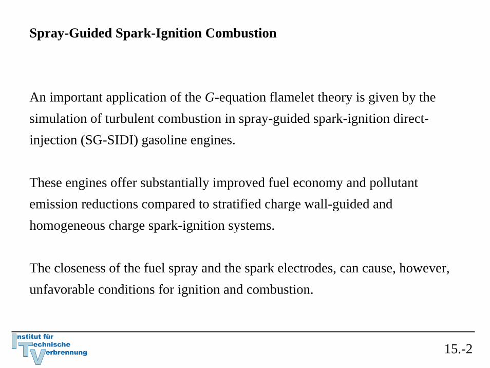
Spray-Guided Spark-Ignition Combustion

An important application of the G-equation flamelet theory is given by the simulation of turbulent combustion in spray-guided spark-ignition direct-injection (SG-SIDI) gasoline engines.

These engines offer substantially improved fuel economy and pollutant emission reductions compared to stratified charge wall-guided and homogeneous charge spark-ignition systems.

The closeness of the fuel spray and the spark electrodes, can cause, however, unfavorable conditions for ignition and combustion.

15.-2

15.-3

(a) Visualization of the mixture preparation process. A detailed 3D numerical simulation of the intake process with a deactivated left intake valve for enhanced swirl generation is performed. The direct fuel spray injection is modeled using a Lagrangian spray model. The spark plug is included in the engine mesh.

(b) Unstructured computational grid (~ 222,000 grid cells) of the engine including the model for the intake runner and the siamese port. (Reprinted with permission by R. Dahms).

A novel development of flamelet models to obtain a more comprehensive understanding of these SG-SIDI ignition processes is presented by the SparkCIMMmodel, recently developed by Dahms et al. (2009).

15.-4

The preparation of the combustible mixture at spark-timing is calculated with a three-dimensional CFD simulation of the gas exchange process, using a standard k-ε turbulence model.

The intake runner, the siamese port, and the spark plug are included in the engine model to capture the interactions of the fuel spray with the spark electrodes (b).

15.-5

The computational grids for the gas exchange and the spray-guided spark-ignition combustion process comprise ~ 222,000 and ~ 97,000 grid cells, respectively.

An enhanced swirl field is generated by the deactivation of the left intake valve (a).

The direct spray-injection is modeled with 25,000 stochastic Lagrangian spray parcels coupled to the gas phase via source terms.

An initial droplet size distribution (SMD=15 μm) is assumed instead of modeling the primary breakup.

More details can be found in Dahms et al. (2009).

15.-6

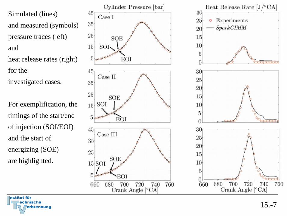
Simulated (lines) and measured (symbols) pressure traces (left) and heat release rates (right) for the investigated cases.

For exemplification, thetimings of the start/end of injection (SOI/EOI) and the start of energizing (SOE) are highlighted.

15.-7

15.-8

3D visualization of fuel spray injection (top row) and turbulent flame front prop-agationfor all investigated cases of the spray-guided gasoline engine.

The applied engine load and mixture dilution result in significant variations of the flame front-averaged value of the turbulent burning velocity in time.

Local flame front values show a substantial deviation from these averaged quantities due to distinctive mixture stratification induced in this engine operating mode.

15.-9

The partially-premixed combustion process of the investigated spray-guided gasoline engine may be classified, using the regime diagram for premixed turbulent combustion by Peters (2000), example for Case III.

15.-10

Although substantial temporal variations of turbulence and flame front velocity and length scales are observed, one recognizes that the operating conditions are located within the thin reaction zone regime throughout the whole combustion process.

This confirms the underlying flamelet assumption of scale separation between the chemical kinetics and the turbulence, and demonstrates the validity of the G-equation flamelet model to predict turbulent partially-premixed combustion in spray-guided spark-ignition direct-injection engines.

15.-11

Investigation of the velocity field close to the spark plug and at spark timing for case II.

15.-12

The flow field results from the direct fuel injection and the gas exchange process, which generates an intensive swirl by the deactivation of the left intake valve.

Local flow velocity magnitudes approach a Favre mean of 50 m/s.

Also steep gradients in the local velocities are shown, indicating high turbulence intensities.

15.-13

High-speed (24,000 frames/s) broadband visible luminosity images of the spark channel for two different individual engine cycles.

15.-14

They show the formation and the turbulent corrugation of the spark channel due to the local high-velocity flow, comparable to the computed velocity

Also, localized ignition spots along the spark channel are observed, which subsequently lead to flame kernel formation and flame front propagation.

Characteristic length scales are identified as the spark channel thickness (~ 0.05 mm)and the flame kernel length scale (~ 0.5 mm).

The spark can stretch up to ~ 10 mm from the spark plug before a restrike occurs.

15.-15

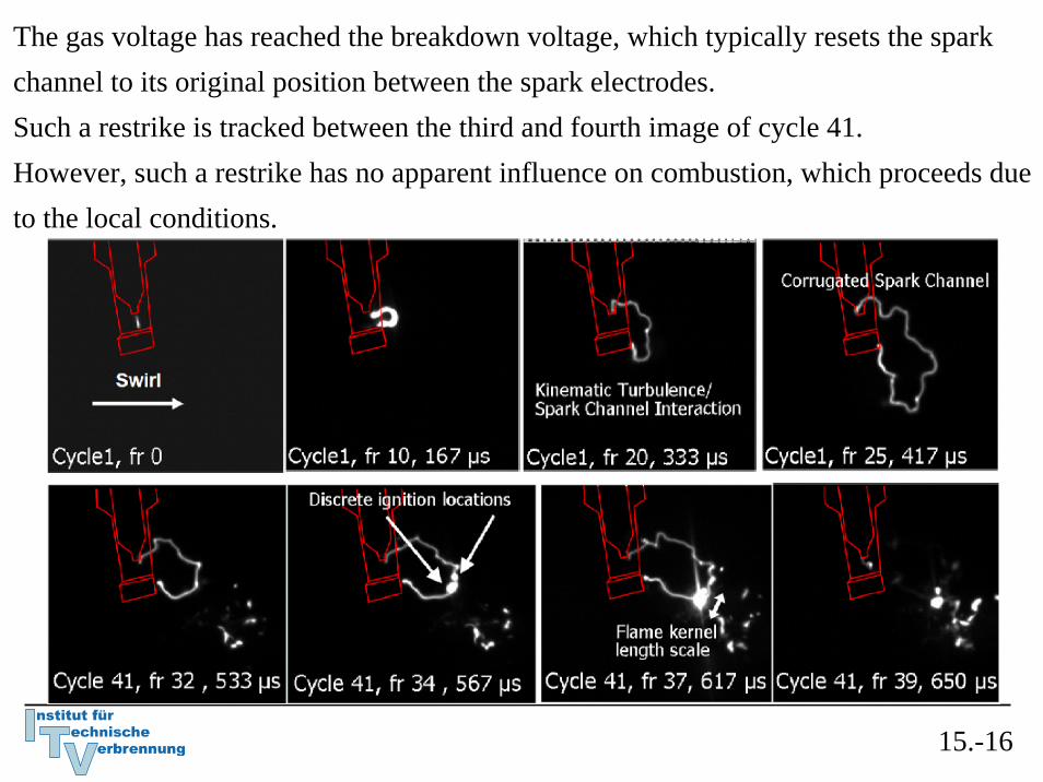
The gas voltage has reached the breakdown voltage, which typically resets the spark channel to its original position between the spark electrodes. Such a restrike is tracked between the third and fourth image of cycle 41. However, such a restrike has no apparent influence on combustion, which proceeds due to the local conditions.

15.-16

The scalar dissipation rates, conditioned on stoichiometric mixture fraction, along this stretched and wrinkled spark channel at ignition timing.

15.-17

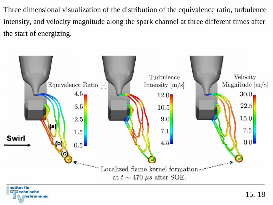
Three dimensional visualization of the distribution of the equivalence ratio, turbulence intensity, and velocity magnitude along the spark channel at three different times after the start of energizing.

15.-18

A side-view comparison of probabilities of finding an instantaneous flame front, - classical single flame kernel model, - high-speed laser-sheet Mie-scattering imaging data- SparkCIMM model

15.-19

A Gaussian distribution of the flame location is used to calculate the flame-location probability for the G-equation simulations.

Without the physical complexity of a detailed spark channel model, the characteristic non-spherical early flame shape cannot be reproduced, which leads to subsequent deficiencies in numerical simulation results.

15.-20

The turbulent Damköhler number, averaged over the early non-spherical mean turbulent flame front after spark advance

15.-21

The initial small Damköhler numbers result from rich and small scale turbulent mixtures, induced by the direct spray injection process, leading to low laminar burning velocities and thick laminar flame thicknesses.

In this regime (red ellipse), the contribution of the turbulence intensity to the turbulent burning velocity is significantly reduced, which in turn largely depends on molecular fuel properties.

15.-22

Injection-Rate Shaping in Diesel Engine Combustion

The concept of flamelet equations and Representative Interactive Flamelets(RIF) prove valuable in the simulation of turbulent combustion in diesel engines.

Here, it is applied to study the effect of top-hat and boot-shaped injection-rate shapes on ignition, combustion, and pollutant formation as an advanced technology to achieve the stringent emission standards in the near future.

15.-23

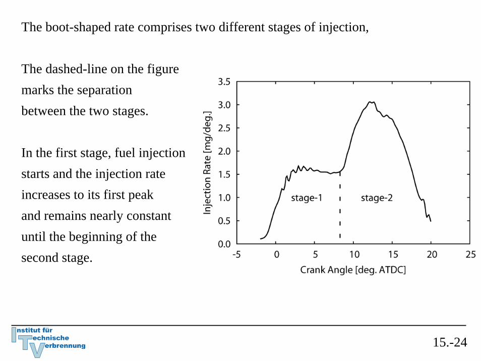
The boot-shaped rate comprises two different stages of injection,

The dashed-line on the figuremarks the separation between the two stages.

In the first stage, fuel injection starts and the injection rate increases to its first peak and remains nearly constant until the beginning of the second stage.

15.-24

In the second stage, the injection rate further increases from the first peak to the second peak, and then decreases till the end of injection time.

The peak injection-rate (referred to as height) in both stages of the boot injection-rate shape is the parameter of variation in this study.

15.-25

Owing to a constant total injected mass and spray momentum (and nearly constant overall injection duration), three different boot-shaped rates.

The figure shows the injection rate (in mg per degree CA) of the investigated boot-shaped rates over crank angle.

The increase in the injectionrates of the first stage meant the decrease in the injection rates of the second stage of a rate shape.

15.-26

The rate shapes are named as BH1, BH2, and BH3 according to their peak injection-rate (height) in the first stage.

Test case BH1 has the lowest peak injection-rate in the first stage and the highest peak injection-rate in the second stage among all.

Whereas, BH3 has the highest peak injection-rate in the first stage and the lowest peak injection-ratein the second stage, respectively.

Test case BH2 is in the middle of BH1 and BH3.

15.-27

Simulations were performed using the multiple-flamelet (M-RIF) model for all the rate shapes.

The contribution of each flamelet in the same computational cell , is calculated from the ratio of its mean mixture fraction and the total value of mixture fraction in the cell.

Turbulent mean values of these scalars are then obtained by using the pre-assumed shape PDF in each cell:

15.-28

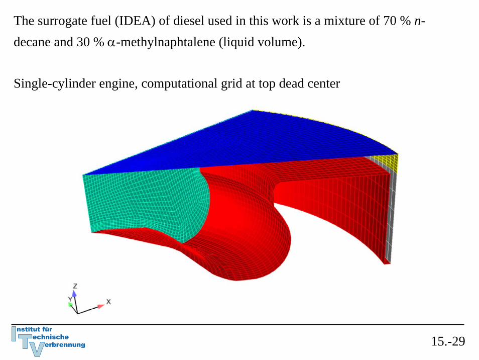
The surrogate fuel (IDEA) of diesel used in this work is a mixture of 70 % n-decane and 30 % α-methylnaphtalene (liquid volume).

Single-cylinder engine, computational grid at top dead center

15.-29

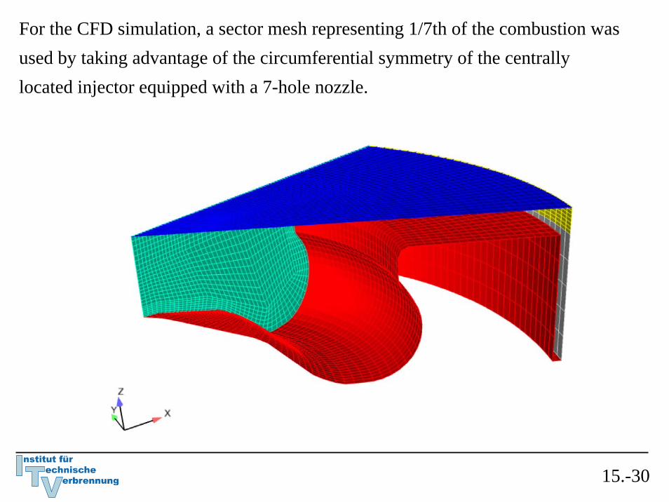
For the CFD simulation, a sector mesh representing 1/7th of the combustion was used by taking advantage of the circumferential symmetry of the centrally located injector equipped with a 7-hole nozzle.

15.-30

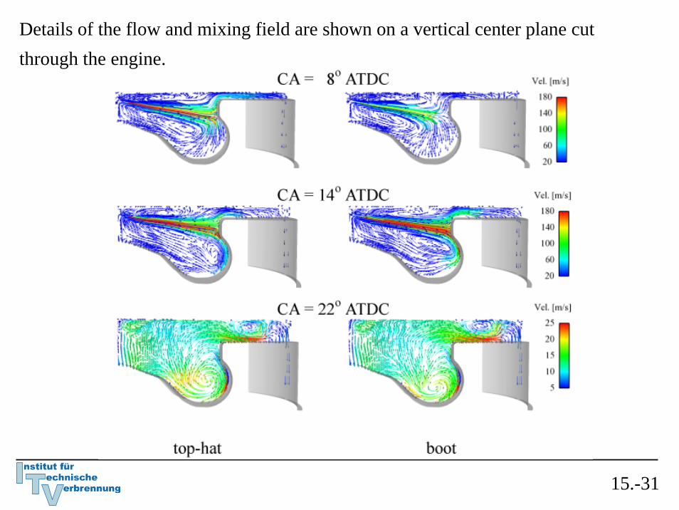
Details of the flow and mixing field are shown on a vertical center plane cut through the engine.

15.-31

The entrainment vortices generated by the spray plume can be clearly observed from the velocity field at 8 oCA ATDC for both rate-shapes.

The piston is traveling down and a strong squish flow is directed into the squish volume (reverse squish) from the piston bowl in both cases of top-hat and boot-shape injection profiles, respectively.

At this crank angle, about 39 % of the total fuel has been injected in the top-hat compared to about 32 % of the total fuel in the boot case.

As a result, the top-hat case has a higher spray center-line velocity.

15.-32

Spatial distributions of the mean mixture fraction

15.-33

In the top-hat, the initial mixing was superior due to the higher velocities (and spray momentum) and hence the vortex has moved deeper inside the bowl and the leading edges of the spray plume are better mixed and leaner compared to the boot case at this crank angle.

15.-34

Thus, in the beginning, the fuel has entered the cylinder with much higher injection velocities in the top-hat, and for the boot shape it happened in the latter crank angles.

A higher transport of fuel for a lower increment in the squish volume results in the richer fuel mixtures in the squish region for the boot case.

At 22 oCA ATDC, a comparison of the mixing field for both shapes shows that the fuel distribution is better for the boot shape allowing the higher mixing with the surrounding air.

15.-35

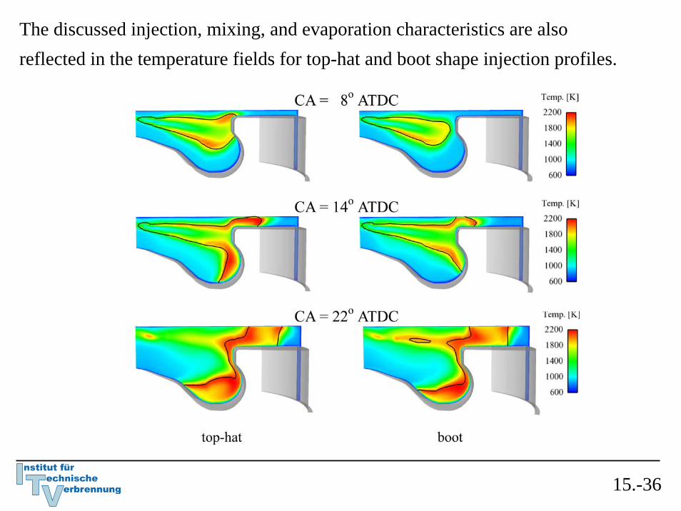
The discussed injection, mixing, and evaporation characteristics are also reflected in the temperature fields for top-hat and boot shape injection profiles.

15.-36

Computed heat release rates for both injection-rate shapes.

The effect of evaporation is evident in the heat release for both shapes.

Earlier start of evaporation in the boot shape shows also early rise in the heat release rates.

The top-hat shape shows the highest premixed peak in heat release rate due to higher evaporation rates during that period. Higher evaporation rates after 10 oCA ATDC in the boot shape results in the highest peak during diffusion-controlled combustion.

15.-37

Comparison of the simulated and measured pressures for both shapes.

The measured and computed pressure evolutions show the same trends and good agreement.

The model predicts an earlier ignition in the boot case as also seen in the experiments.

This trend could be associated with the early start of injection and fuel evaporation leading to early molecular level mixing for the boot case.

15.-38

Comparison of the simulated and measured soot (top) and CO (below) emissions at exhaust valve opening (EVO).

The indicated concentrations are scaled to one in the top-hat case.Similar to the experiments, the model predicts a significant reduction in both soot and CO emissions at EVO for the boot shape.

15.-39

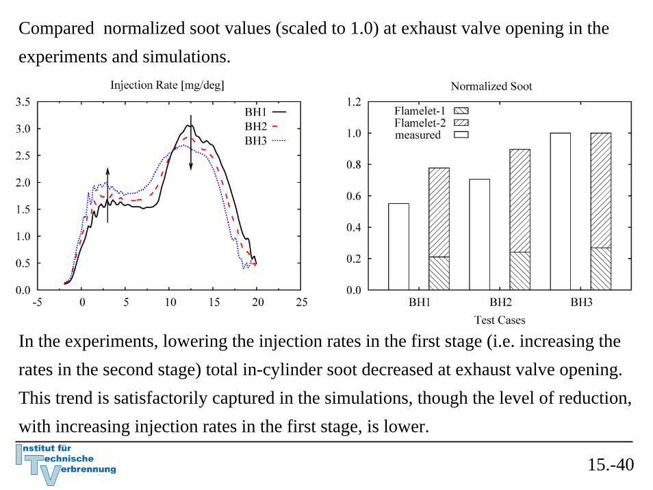
Compared normalized soot values (scaled to 1.0) at exhaust valve opening in the experiments and simulations.

In the experiments, lowering the injection rates in the first stage (i.e. increasing the rates in the second stage) total in-cylinder soot decreased at exhaust valve opening. This trend is satisfactorily captured in the simulations, though the level of reduction, with increasing injection rates in the first stage, is lower.

15.-40

History of soot formation for the mass belonging to the first stage.

BH3 has the lowest, and BH1 has the highest peak soot formation.

One can conclude that the higher injection rates in the first stage results in a lower peak in soot formation.

15.-41

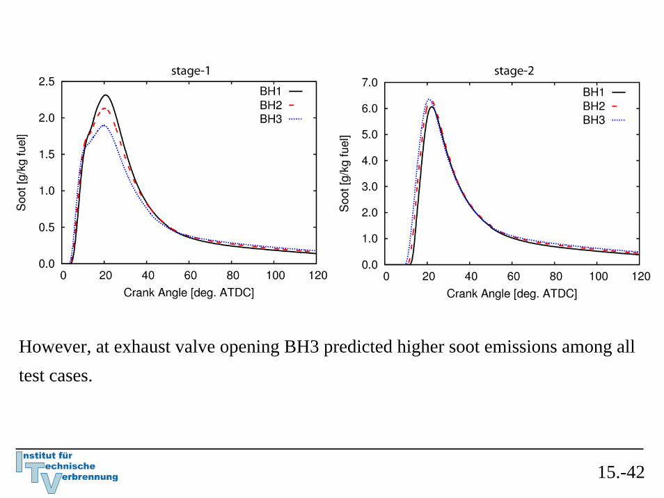
However, at exhaust valve opening BH3 predicted higher soot emissions among all test cases.

15.-42

The rate shape corresponding to BH1 shows the improved soot oxidation among the rate shapes.

15.-43