lecture 14 - stanford university
TRANSCRIPT
1
Intermediate Code & Local Optimizations
Lecture 14
Instructor: Fredrik KjolstadSlide design by Prof. Alex Aiken, with modifications
2
Lecture Outline
• Intermediate code
• Local optimizations
• Next time: global optimizations
3
Code Generation Summary
• We have discussed– Runtime organization– Simple stack machine code generation– Improvements to stack machine code generation
• Our compiler maps AST to assembly language– And does not perform optimizations
4
Optimization
• Optimization is our last compiler phase
• Most complexity in modern compilers is in the optimizer– Also by far the largest phase
• First, we need to discuss intermediate languages
5
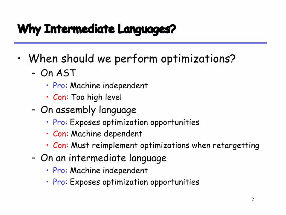
Why Intermediate Languages?
• When should we perform optimizations?– On AST
• Pro: Machine independent• Con: Too high level
– On assembly language• Pro: Exposes optimization opportunities• Con: Machine dependent• Con: Must reimplement optimizations when retargetting
– On an intermediate language• Pro: Machine independent• Pro: Exposes optimization opportunities
6
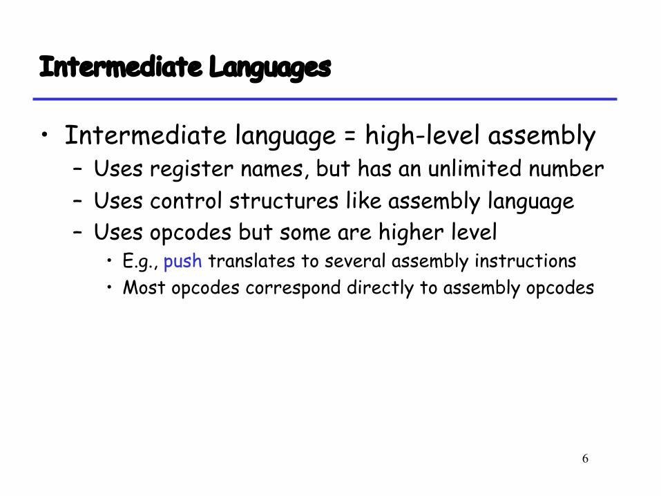
Intermediate Languages
• Intermediate language = high-level assembly – Uses register names, but has an unlimited number– Uses control structures like assembly language– Uses opcodes but some are higher level
• E.g., push translates to several assembly instructions• Most opcodes correspond directly to assembly opcodes
7
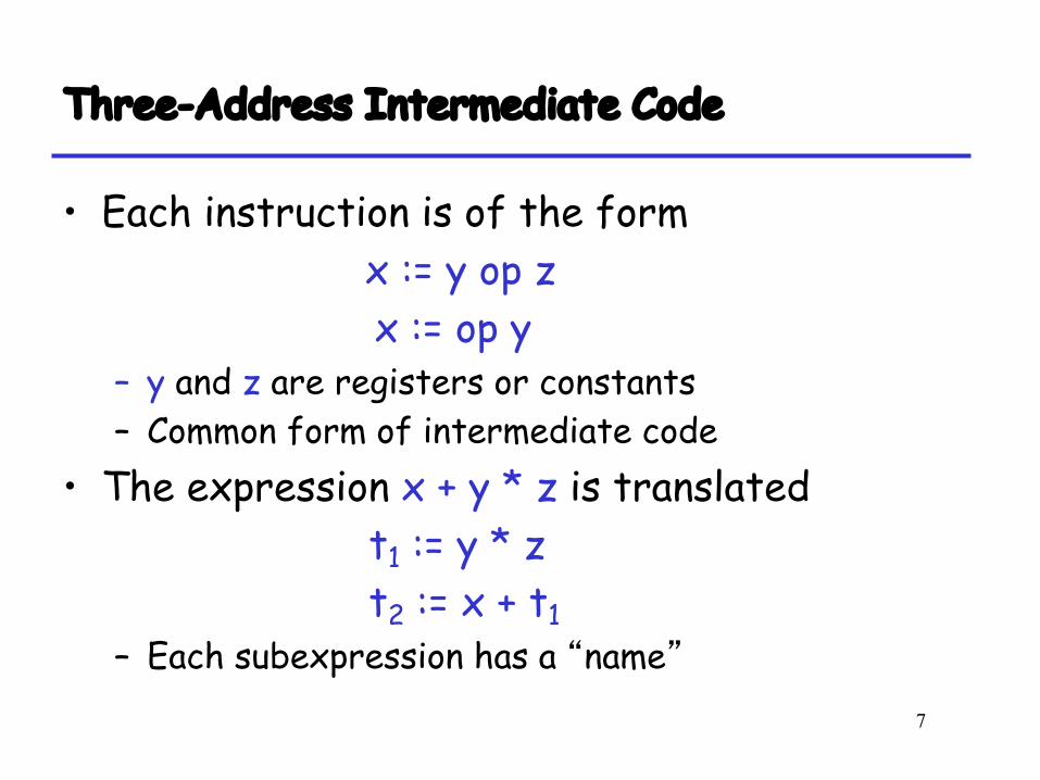
Three-Address Intermediate Code
• Each instruction is of the formx := y op zx := op y
– y and z are registers or constants– Common form of intermediate code
• The expression x + y * z is translatedt1 := y * zt2 := x + t1
– Each subexpression has a “name”
8
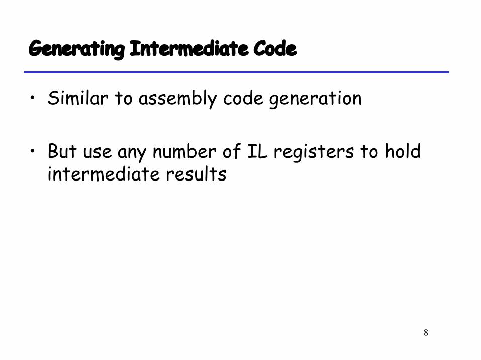
Generating Intermediate Code
• Similar to assembly code generation
• But use any number of IL registers to hold intermediate results
9
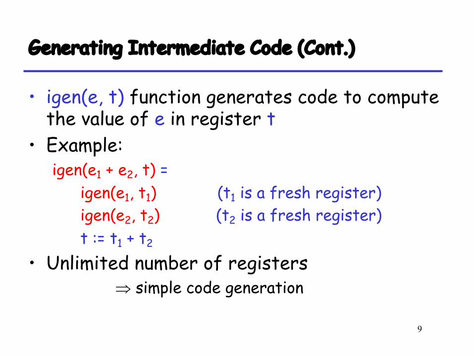
Generating Intermediate Code (Cont.)
• igen(e, t) function generates code to compute the value of e in register t
• Example:igen(e1 + e2, t) =
igen(e1, t1) (t1 is a fresh register)igen(e2, t2) (t2 is a fresh register)t := t1 + t2
• Unlimited number of registersÞ simple code generation
10
Intermediate Code Notes
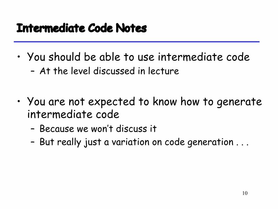
• You should be able to use intermediate code– At the level discussed in lecture
• You are not expected to know how to generate intermediate code– Because we won’t discuss it– But really just a variation on code generation . . .
11
An Intermediate Language
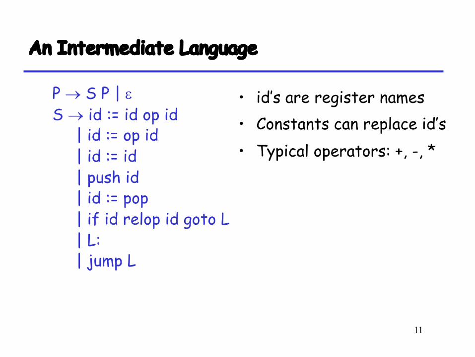
P ® S P | eS ® id := id op id
| id := op id| id := id| push id| id := pop| if id relop id goto L| L:| jump L
• id’s are register names• Constants can replace id’s• Typical operators: +, -, *
12
Definition. Basic Blocks
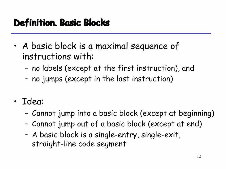
• A basic block is a maximal sequence of instructions with: – no labels (except at the first instruction), and – no jumps (except in the last instruction)
• Idea: – Cannot jump into a basic block (except at beginning)– Cannot jump out of a basic block (except at end)– A basic block is a single-entry, single-exit,
straight-line code segment
13
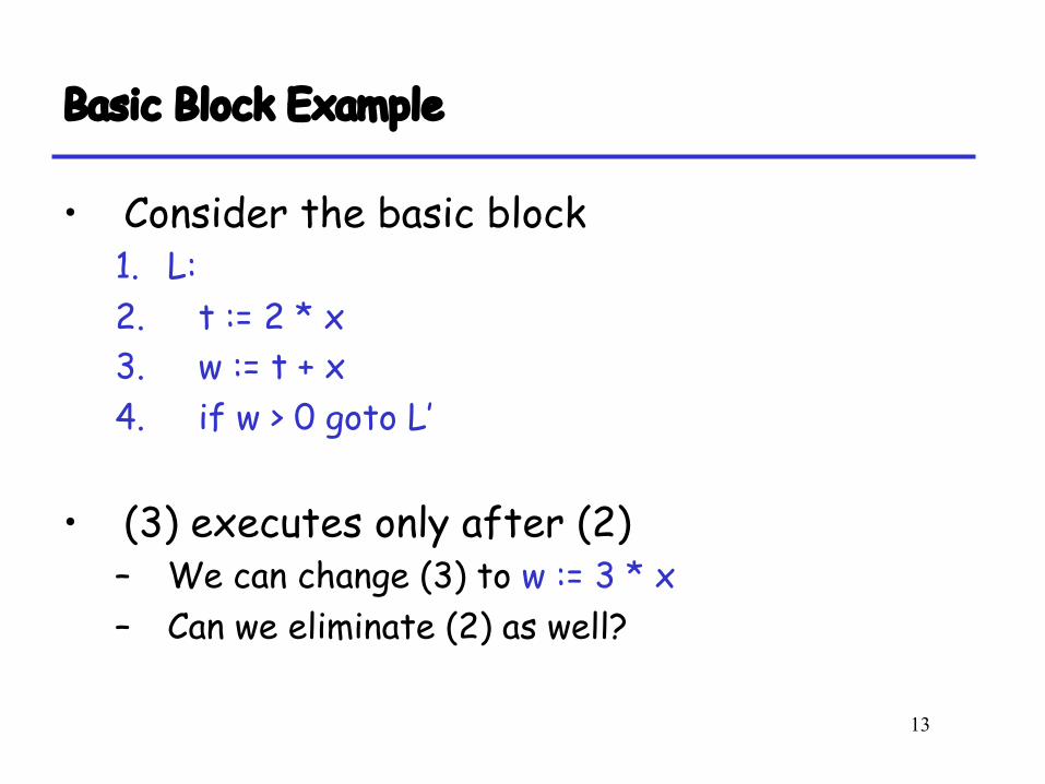
Basic Block Example
• Consider the basic block1. L: 2. t := 2 * x3. w := t + x4. if w > 0 goto L’
• (3) executes only after (2) – We can change (3) to w := 3 * x– Can we eliminate (2) as well?
14
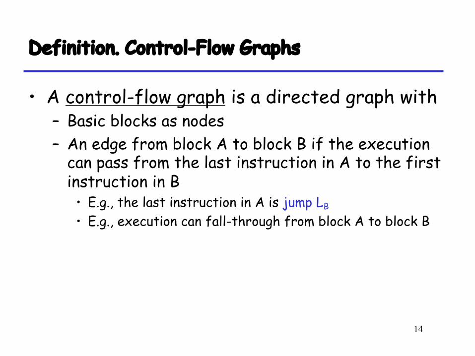
Definition. Control-Flow Graphs
• A control-flow graph is a directed graph with– Basic blocks as nodes– An edge from block A to block B if the execution
can pass from the last instruction in A to the first instruction in B
• E.g., the last instruction in A is jump LB
• E.g., execution can fall-through from block A to block B
15
Example of Control-Flow Graphs
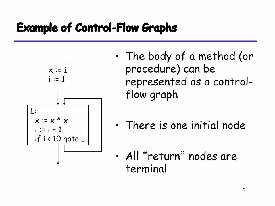
• The body of a method (or procedure) can be represented as a control-flow graph
• There is one initial node
• All “return” nodes are terminal
x := 1i := 1
L:x := x * xi := i + 1if i < 10 goto L
16
Optimization Overview
• Optimization seeks to improve a program’s resource utilization– Execution time (most often)– Code size– Network messages sent, etc.
• Optimization should not alter what the program computes– The answer must still be the same
17
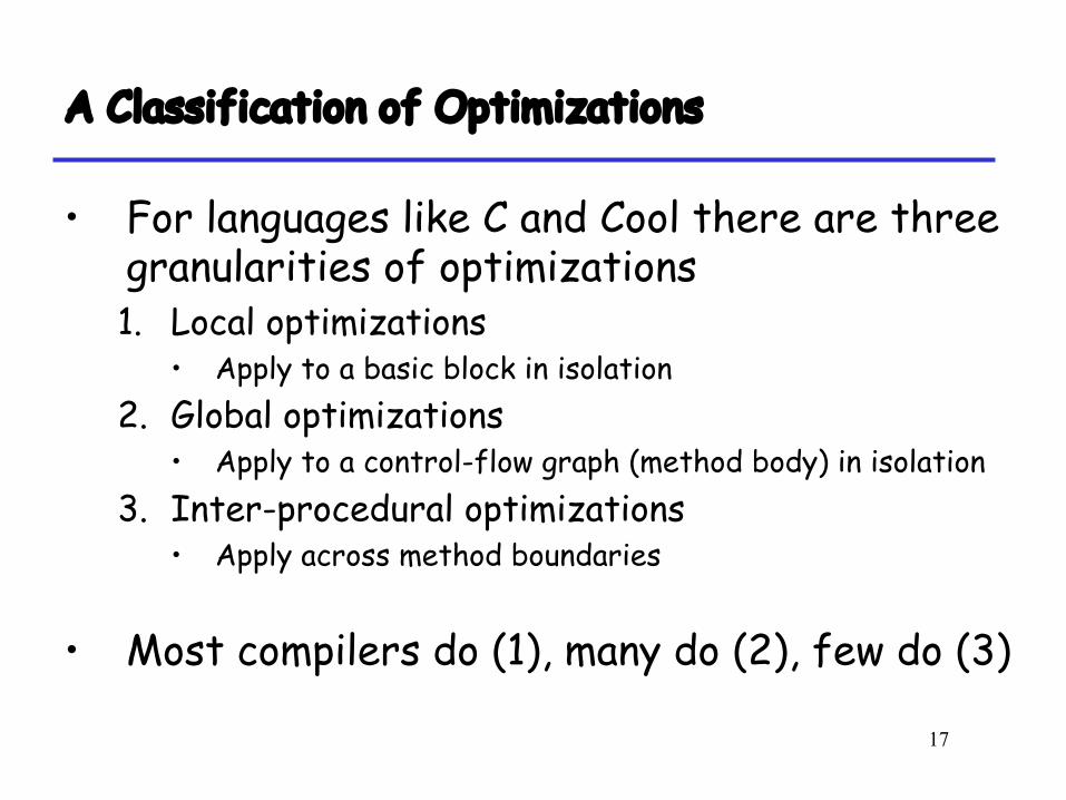
A Classification of Optimizations
• For languages like C and Cool there are three granularities of optimizations1. Local optimizations
• Apply to a basic block in isolation2. Global optimizations
• Apply to a control-flow graph (method body) in isolation3. Inter-procedural optimizations
• Apply across method boundaries
• Most compilers do (1), many do (2), few do (3)
18
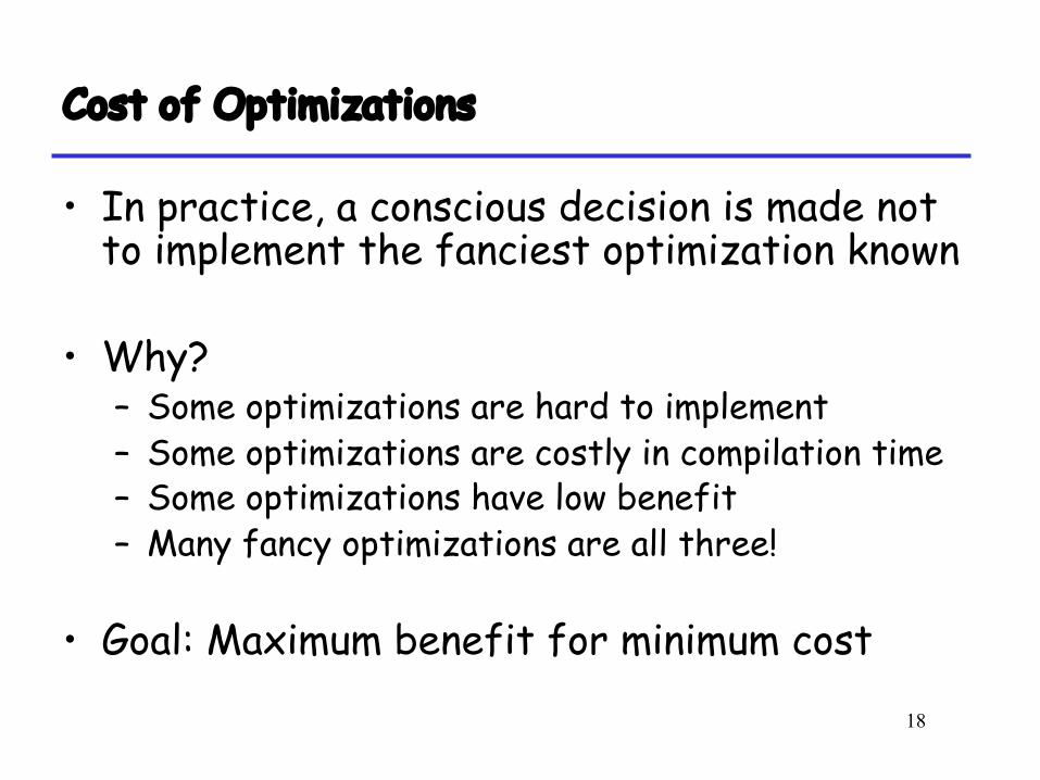
Cost of Optimizations
• In practice, a conscious decision is made not to implement the fanciest optimization known
• Why?– Some optimizations are hard to implement– Some optimizations are costly in compilation time– Some optimizations have low benefit– Many fancy optimizations are all three!
• Goal: Maximum benefit for minimum cost
19
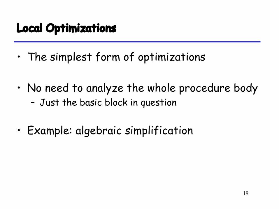
Local Optimizations
• The simplest form of optimizations
• No need to analyze the whole procedure body– Just the basic block in question
• Example: algebraic simplification
20
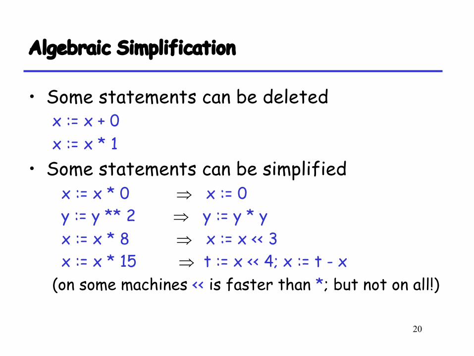
Algebraic Simplification
• Some statements can be deletedx := x + 0x := x * 1
• Some statements can be simplifiedx := x * 0 Þ x := 0y := y ** 2 Þ y := y * yx := x * 8 Þ x := x << 3x := x * 15 Þ t := x << 4; x := t - x
(on some machines << is faster than *; but not on all!)
21
Constant Folding
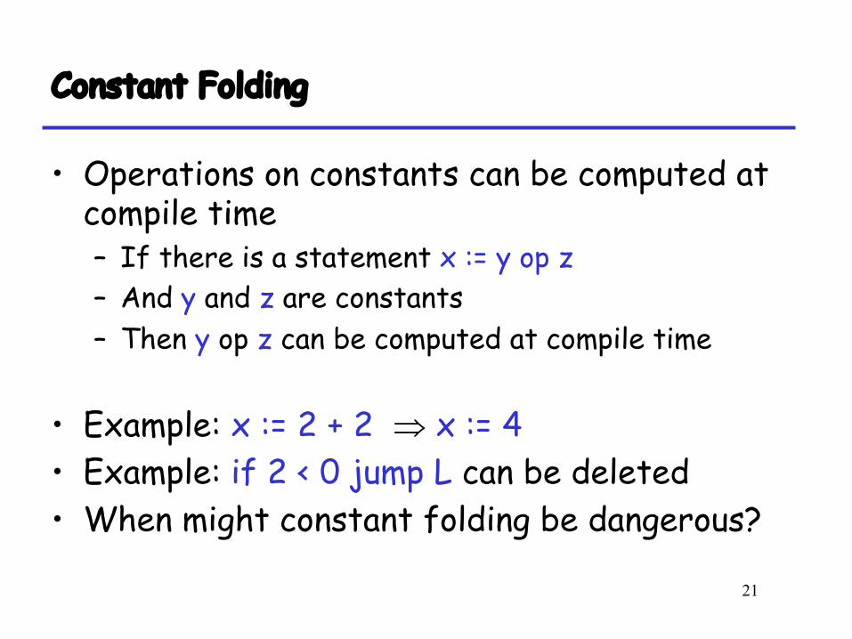
• Operations on constants can be computed at compile time– If there is a statement x := y op z– And y and z are constants– Then y op z can be computed at compile time
• Example: x := 2 + 2 Þ x := 4• Example: if 2 < 0 jump L can be deleted• When might constant folding be dangerous?
22
Flow of Control Optimizations
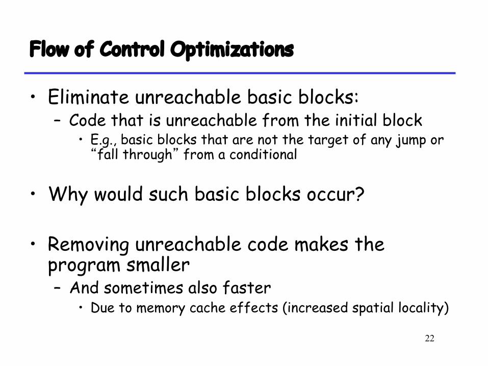
• Eliminate unreachable basic blocks:– Code that is unreachable from the initial block
• E.g., basic blocks that are not the target of any jump or “fall through” from a conditional
• Why would such basic blocks occur?
• Removing unreachable code makes the program smaller– And sometimes also faster
• Due to memory cache effects (increased spatial locality)
23
Static Single Assignment (SSA) Form
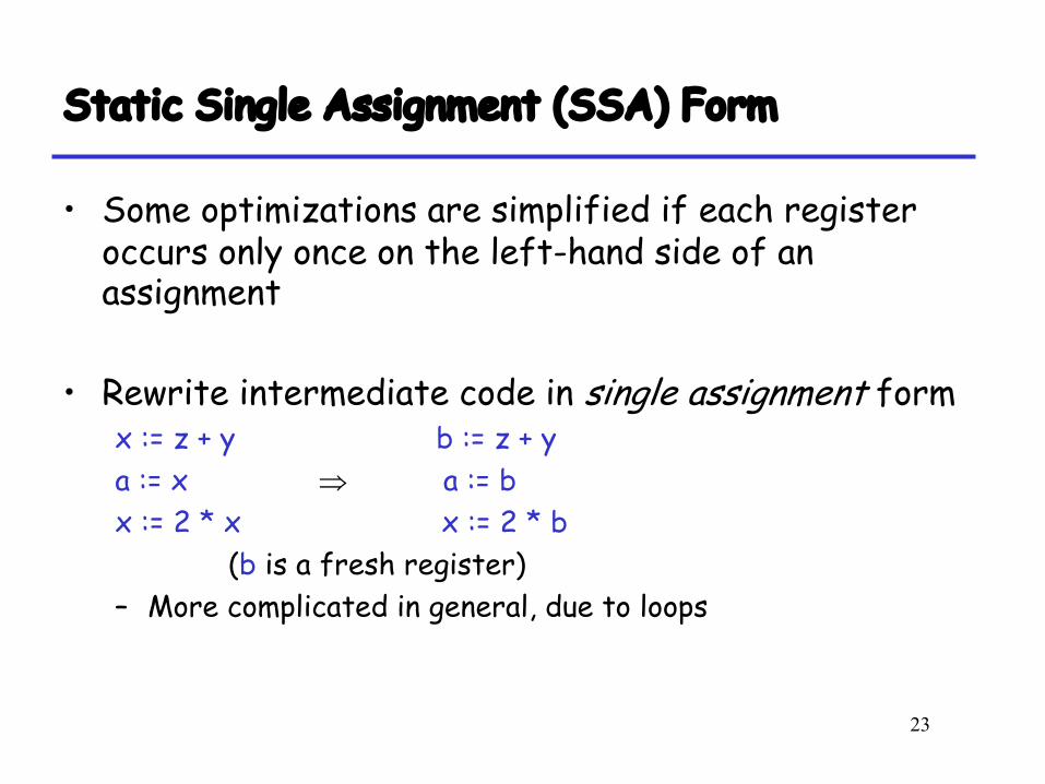
• Some optimizations are simplified if each register occurs only once on the left-hand side of an assignment
• Rewrite intermediate code in single assignment formx := z + y b := z + ya := x Þ a := bx := 2 * x x := 2 * b
(b is a fresh register)– More complicated in general, due to loops
24
Common Subexpression Elimination
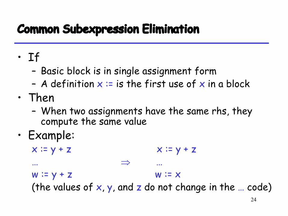
• If– Basic block is in single assignment form– A definition x := is the first use of x in a block
• Then– When two assignments have the same rhs, they
compute the same value• Example:
x := y + z x := y + z… Þ …w := y + z w := x(the values of x, y, and z do not change in the … code)
25
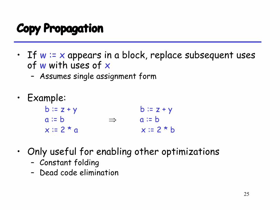
Copy Propagation
• If w := x appears in a block, replace subsequent uses of w with uses of x– Assumes single assignment form
• Example:b := z + y b := z + ya := b Þ a := bx := 2 * a x := 2 * b
• Only useful for enabling other optimizations– Constant folding– Dead code elimination
26
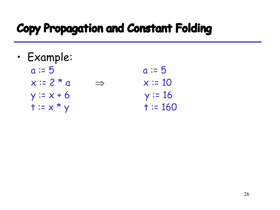
Copy Propagation and Constant Folding
• Example:a := 5 a := 5x := 2 * a Þ x := 10y := x + 6 y := 16t := x * y t := 160
27
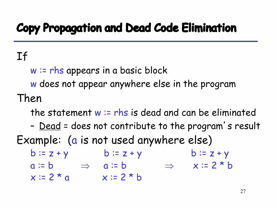
Copy Propagation and Dead Code Elimination
If w := rhs appears in a basic blockw does not appear anywhere else in the program
Then the statement w := rhs is dead and can be eliminated– Dead = does not contribute to the program’s result
Example: (a is not used anywhere else)b := z + y b := z + y b := z + ya := b Þ a := b Þ x := 2 * bx := 2 * a x := 2 * b
28
Applying Local Optimizations
• Each local optimization does little by itself
• Typically optimizations interact– Performing one optimization enables another
• Optimizing compilers repeat optimizations until no improvement is possible– The optimizer can also be stopped at any point to
limit compilation time
29
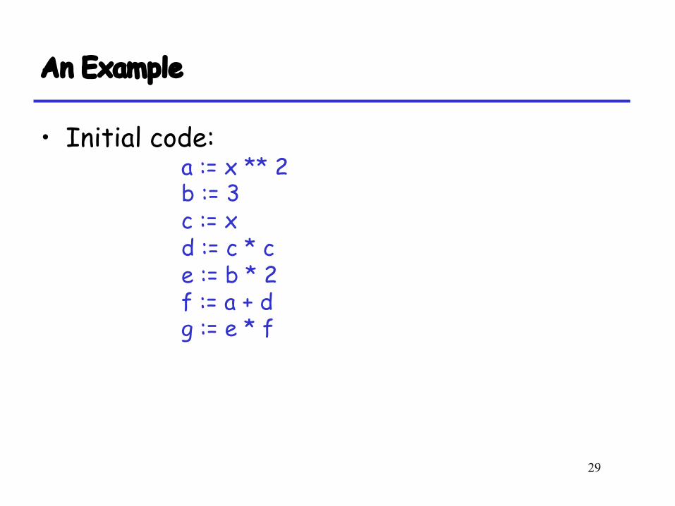
An Example
• Initial code:a := x ** 2 b := 3c := xd := c * ce := b * 2 f := a + dg := e * f

30
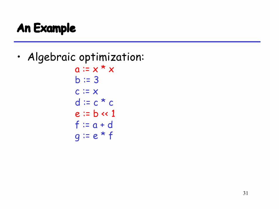
An Example
• Algebraic optimization:a := x ** 2b := 3c := xd := c * ce := b * 2f := a + dg := e * f
31
An Example
• Algebraic optimization:a := x * xb := 3c := xd := c * ce := b << 1f := a + dg := e * f
32
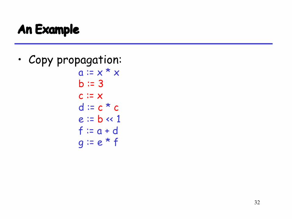
An Example
• Copy propagation:a := x * x b := 3c := xd := c * ce := b << 1 f := a + dg := e * f
33
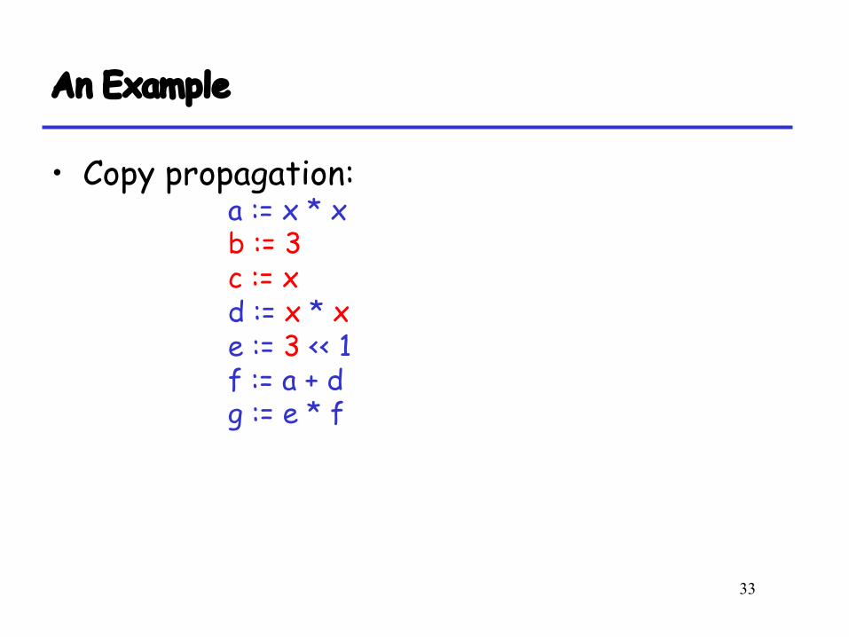
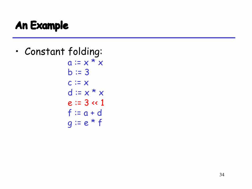
An Example
• Copy propagation:a := x * x b := 3c := xd := x * xe := 3 << 1 f := a + dg := e * f
34
An Example
• Constant folding:a := x * x b := 3c := xd := x * xe := 3 << 1f := a + dg := e * f
35
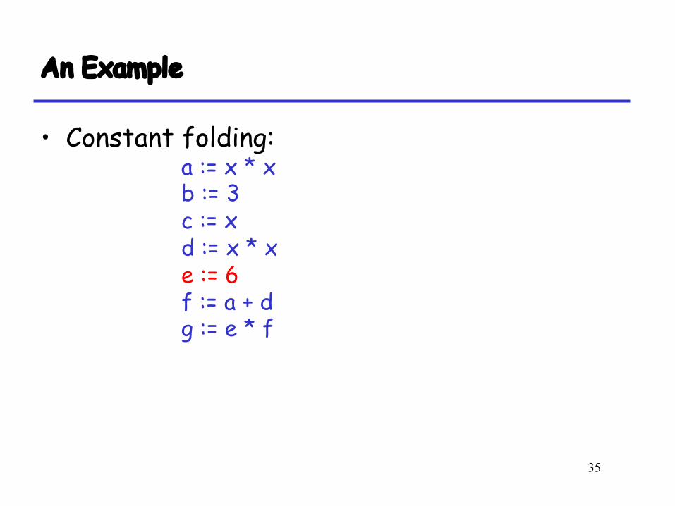
An Example
• Constant folding:a := x * x b := 3c := xd := x * xe := 6f := a + dg := e * f
36
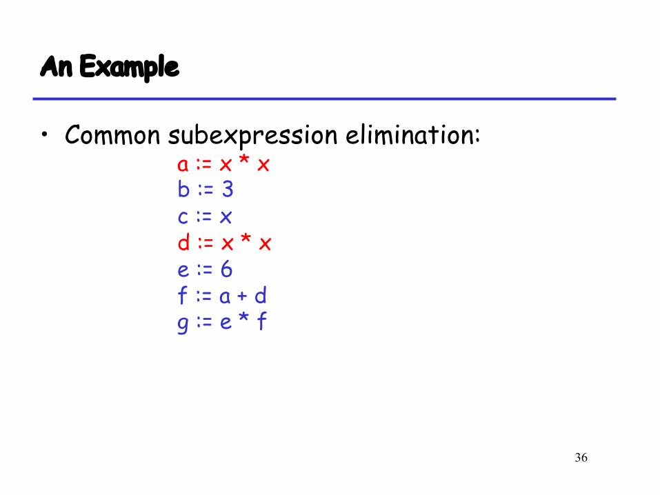
An Example
• Common subexpression elimination:a := x * xb := 3c := xd := x * xe := 6 f := a + dg := e * f
37
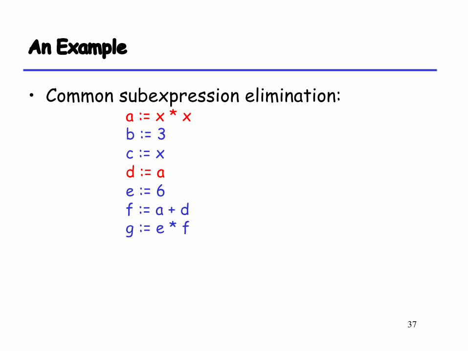
An Example
• Common subexpression elimination:a := x * xb := 3c := xd := ae := 6 f := a + dg := e * f
38
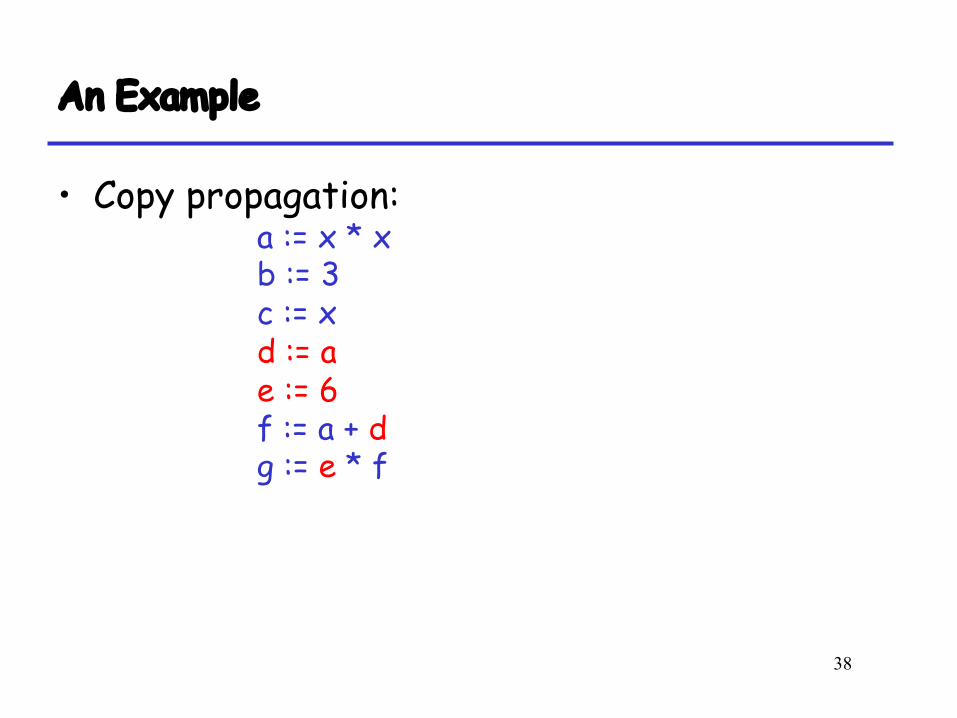
An Example
• Copy propagation:a := x * x b := 3c := xd := ae := 6f := a + dg := e * f
Prof. Aiken CS 143 Lecture 14 39
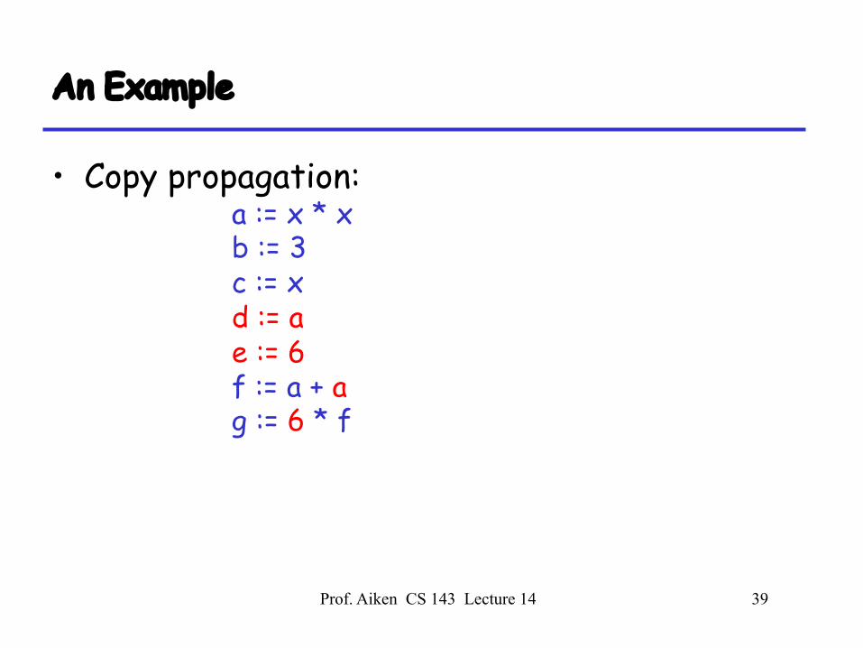
An Example
• Copy propagation:a := x * x b := 3c := xd := ae := 6f := a + ag := 6 * f
40
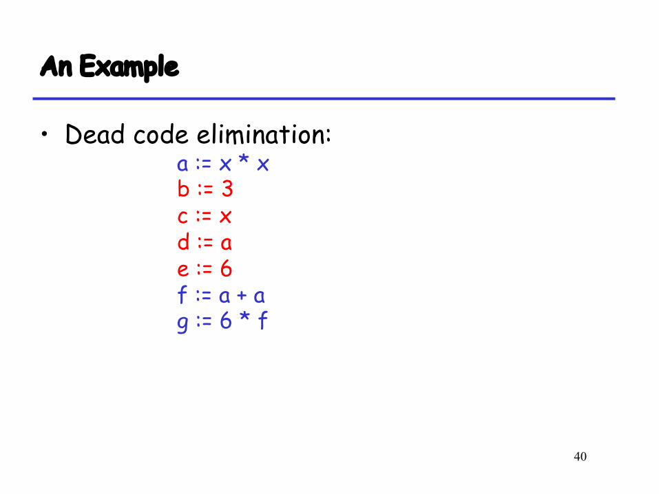
An Example
• Dead code elimination:a := x * x b := 3c := xd := ae := 6f := a + ag := 6 * f
41
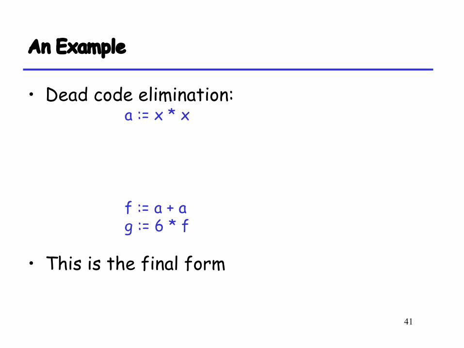
An Example
• Dead code elimination:a := x * x
f := a + ag := 6 * f
• This is the final form
42
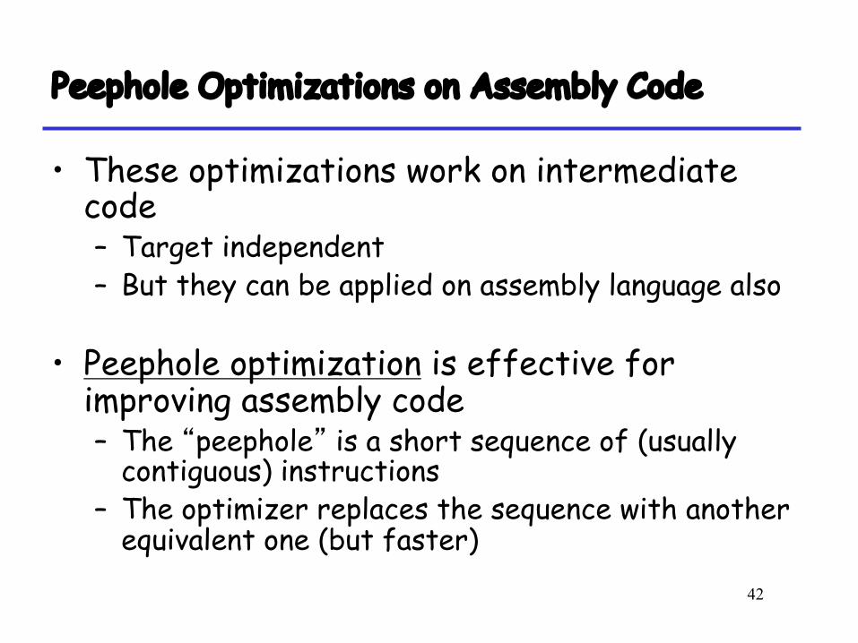
Peephole Optimizations on Assembly Code
• These optimizations work on intermediate code– Target independent– But they can be applied on assembly language also
• Peephole optimization is effective for improving assembly code– The “peephole” is a short sequence of (usually
contiguous) instructions– The optimizer replaces the sequence with another
equivalent one (but faster)
43
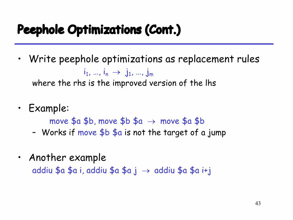
Peephole Optimizations (Cont.)
• Write peephole optimizations as replacement rulesi1, …, in ® j1, …, jm
where the rhs is the improved version of the lhs
• Example:move $a $b, move $b $a ® move $a $b
– Works if move $b $a is not the target of a jump
• Another exampleaddiu $a $a i, addiu $a $a j ® addiu $a $a i+j
44
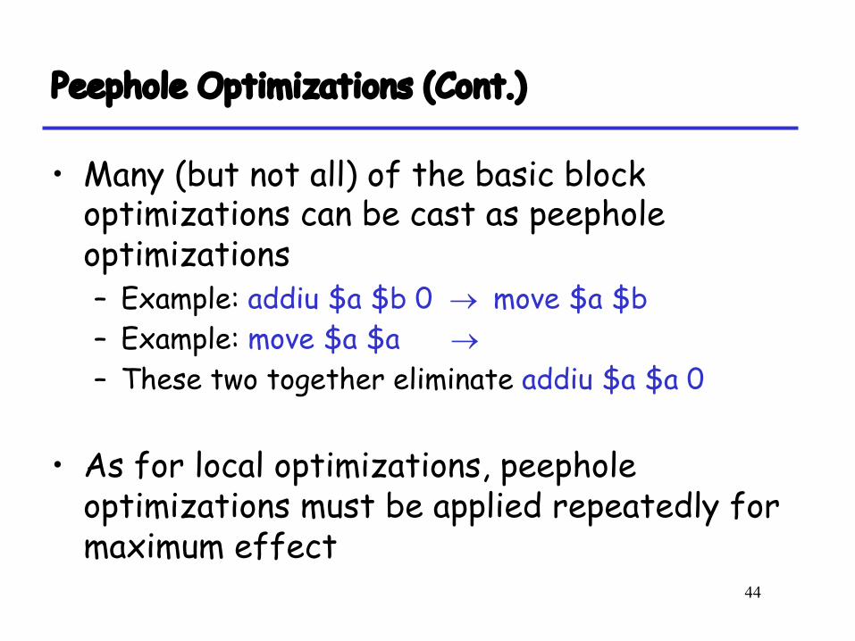
Peephole Optimizations (Cont.)
• Many (but not all) of the basic block optimizations can be cast as peephole optimizations– Example: addiu $a $b 0 ® move $a $b– Example: move $a $a ®– These two together eliminate addiu $a $a 0
• As for local optimizations, peephole optimizations must be applied repeatedly for maximum effect
45
Local Optimizations: Notes
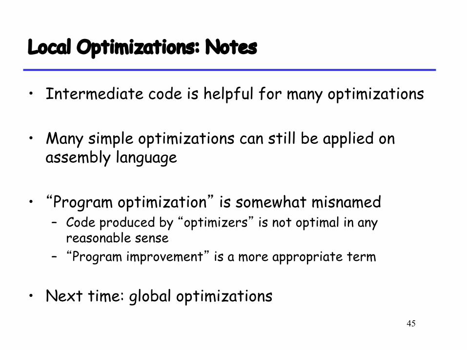
• Intermediate code is helpful for many optimizations
• Many simple optimizations can still be applied on assembly language
• “Program optimization” is somewhat misnamed– Code produced by “optimizers” is not optimal in any
reasonable sense– “Program improvement” is a more appropriate term
• Next time: global optimizations