Lecture 13: Images as Compositions of Patterns

A.L. Yuille

March 13, 2012

1 Introduction

Pattern theory is a research program which believes that visual processing is best thought of in termsof patterns (Grenander 1973, Mumford and Desolneux 2010). Images can be expressed as combinationsof elementary patterns, see figure (1), and image interpretation/understanding consists of decomposing theimage into these patterns. The same principles apply to other sensory systems and to cognition and thought.This program is very attractive but it is also very difficult. Here we restrict ourself to applying it to imagesegmentation with a small extension to image parsing which includes the detection and recognition of objects.Note that the weak membrane/smooth models of images (earlier lectures) can be thought of as examples ofthis approach but where the patterns are very simple – image regions with smooth intensity. The patterntheory approach suggests that we have a larger dictionary of patterns – including texture, shading, and evenpatterns for objects such as faces and text. See also Zhu and Mumford (2006).

a football match scene

texture

text

face

person

color region

curve groupstexture

sports field spectator

texture

persons

point process

Figure 1: Pattern theory argues that images are composed from different patterns and the task of imageprocessing is to parse the image into its constituent patterns.

This lecture will start by describing snakes (Witkin, Terzopoulos, Kass) which relate to this frameworkbut pre-date it. This is one of the most cited papers in computer vision. We will formulate it probabilistically,which relates to a model for detecting roads by Geman and Jedynak.

After describing snakes, we will proceed by describing three pattern theory models of images of increasingcomplexity: (i) Zhu and Yuille (1996), (ii) Tu and Zhu (2002), and (iii) Tu, Chen, Yuille, Zhu (2005). The

1

last two require complex algorithms – data driven Markov Chain Monte Carlo (DDMCMC), which we willalso describe. We will introduce (ii) and (iii) together since the mathematics is very similar.

2 Snakes

Snakes were originally intended as an interactive tool. It has many applications and, in particular, itmotivated considerable work on object tracking (see ”Active Vision” A. Blake and A.L. Yuille eds.).

2.1 Basic Snakes

A snake is a contour by Γ(s) (s is not the arc length). Typically Γ(s) is a closed contour. It is defined by anenergy function:

E[Γ] =

∫Γ

1

2α|~Γs(s)|2 + β|~Γss|2 − λ|~∇I(~x(s))|2ds. (1)

Here s denotes partial derivative with respect to s – Γs = ∂~Γ∂s .

To run a snake, you initialize it by placing it near, or surrounding, and object (e.g. a face). Thenminimize E[Γ] by steepest descent. This gives update equations:

d~Γ(s)

dt= −α~Γss + β~Γssss + λ~∇|~∇I|2. (2)

The first two terms try to make the curve short and have small curvature (NEED AN APPENDIX ONCURVATURE.). The third term tries to move the snake to regions of large intensity gradient.

Snakes can be modified in several different ways. Basic snakes try to minimize their areas (consequenceof the prior terms). But we can have balloons by putting in prior terms that try to make the area as bigas possible. We can also add regional terms (check Ishihara and Geiger!!). Alternative algorithms are moreeffective than steepest descent.

2.2 Bayesian Interpretation of Snakes

Bayesian interpretation. There is a natural Bayesian interpretation of snakes. This shows that the energyimaging term −|~∇I|2 is not very sensible (as was realized in practice fairly soon). Technically this requirestaking the continuous formulation and discretizing it.

Specify a generative model for the image intensity gradients (see notes for lecture 1):

P (|~∇I||Γ) =∏~x∈Γ

Pon(|~∇I(~x)|)∏

~x∈Ω/Γ

Poff (|~∇I(~x)|). (3)

P (Γ) =1

Zexp−

∫Γ

1

2α|~Γs(s)|2 + β|~Γss|2. (4)

MAP estimation of Γ corresponds to minimizing:

− logP (|~∇I||Γ)− logP (Γ), (5)

where we see that the second term reduces to the spatial terms in the energy function for the snakes.We now concentrate on the first term which can be re-expressed as:

−∑~x∈Γ

logPon(|~∇I(~x)|)−∑~x∈Ω/Γ

logPoff (|~∇I(~x)|) = −∑~x∈Γ

logPon(|~∇I(~x)|)Poff (|~∇I(~x)|)

−∑~x∈Ω

Poff (|~∇I(~x)|). (6)

2

We see that the second term is independent of Γ and hence can be dropped during MAP estimation. We

then see that log Pon(|~∇I(~x)|)Poff (|~∇I(~x)|)

corresponds to the term −|~∇I(~x)|2. But we know what the typical shape of

the log-likelihood function is from lecture 1 – and it certainly is not −|~∇I(~x)|2! Instead it rises slowly from

a minimum at |~∇I| = 0 and (roughly) asymptotes. This is because if |~∇I| is large then it is almost certainly

an edge – but −|~∇I(~x)|2 rewards big edges too much at the expense of small edges.Models like equation (6) were used, in combination with a smoothness prior, to model roads in aerial

images (Geman and Jedynak).

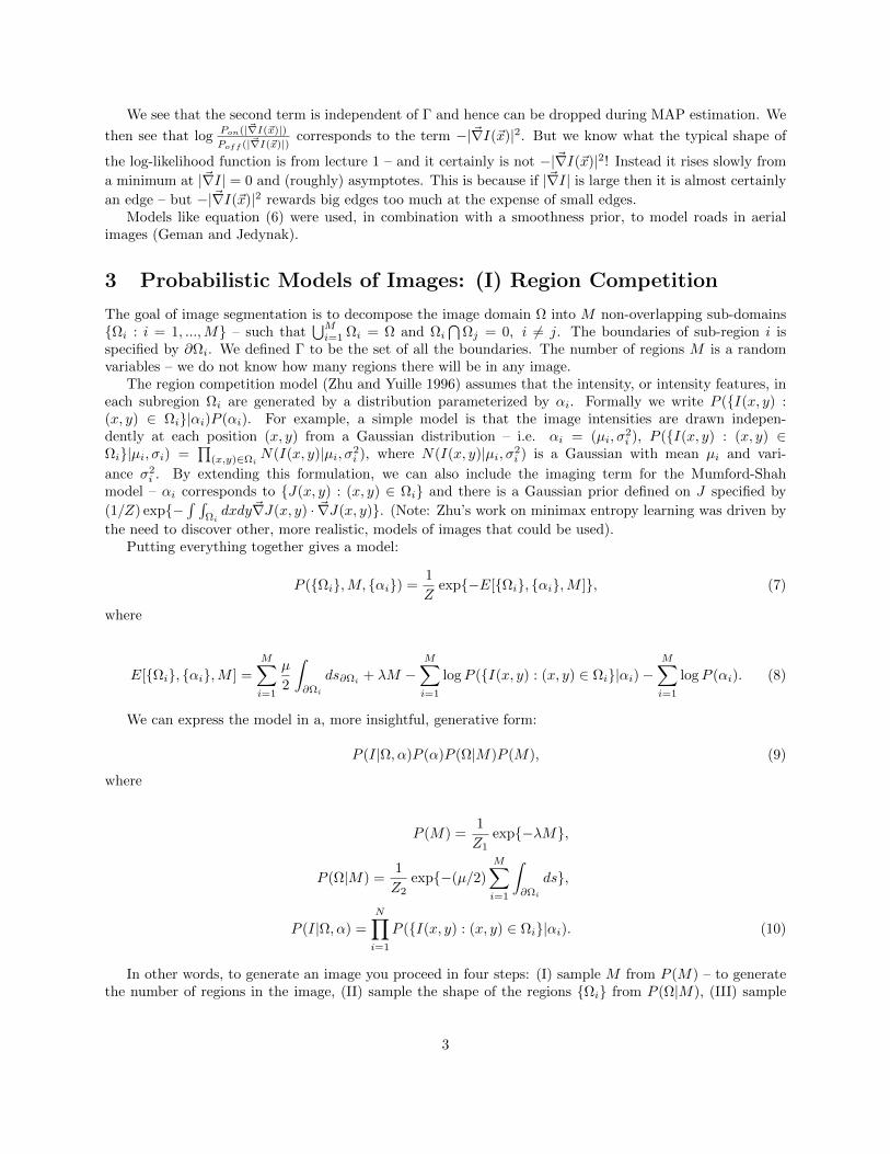
3 Probabilistic Models of Images: (I) Region Competition

The goal of image segmentation is to decompose the image domain Ω into M non-overlapping sub-domainsΩi : i = 1, ...,M – such that

⋃Mi=1 Ωi = Ω and Ωi

⋂Ωj = 0, i 6= j. The boundaries of sub-region i is

specified by ∂Ωi. We defined Γ to be the set of all the boundaries. The number of regions M is a randomvariables – we do not know how many regions there will be in any image.

The region competition model (Zhu and Yuille 1996) assumes that the intensity, or intensity features, ineach subregion Ωi are generated by a distribution parameterized by αi. Formally we write P (I(x, y) :(x, y) ∈ Ωi|αi)P (αi). For example, a simple model is that the image intensities are drawn indepen-dently at each position (x, y) from a Gaussian distribution – i.e. αi = (µi, σ

2i ), P (I(x, y) : (x, y) ∈

Ωi|µi, σi) =∏

(x,y)∈ΩiN(I(x, y)|µi, σ2

i ), where N(I(x, y)|µi, σ2i ) is a Gaussian with mean µi and vari-

ance σ2i . By extending this formulation, we can also include the imaging term for the Mumford-Shah

model – αi corresponds to J(x, y) : (x, y) ∈ Ωi and there is a Gaussian prior defined on J specified by

(1/Z) exp−∫ ∫

Ωidxdy~∇J(x, y) · ~∇J(x, y). (Note: Zhu’s work on minimax entropy learning was driven by

the need to discover other, more realistic, models of images that could be used).Putting everything together gives a model:

P (Ωi,M, αi) =1

Zexp−E[Ωi, αi,M ], (7)

where

E[Ωi, αi,M ] =

M∑i=1

µ

2

∫∂Ωi

ds∂Ωi + λM −M∑i=1

logP (I(x, y) : (x, y) ∈ Ωi|αi)−M∑i=1

logP (αi). (8)

We can express the model in a, more insightful, generative form:

P (I|Ω, α)P (α)P (Ω|M)P (M), (9)

where

P (M) =1

Z1exp−λM,

P (Ω|M) =1

Z2exp−(µ/2)

M∑i=1

∫∂Ωi

ds,

P (I|Ω, α) =

N∏i=1

P (I(x, y) : (x, y) ∈ Ωi|αi). (10)

In other words, to generate an image you proceed in four steps: (I) sample M from P (M) – to generatethe number of regions in the image, (II) sample the shape of the regions Ωi from P (Ω|M), (III) sample

3

the parameters αi for each region from P (α), and (IV) sample the images in each region from P (I(x, y) :(x, y) ∈ Ωi|αi).

In practice, it is very hard to do this sampling. The most difficult step is to sample from P (Ω|M) togenerate a partition of the image into regions (there have been few attempts to do this). But, using themore advanced model in the next section, Tu and Zhu (2002) did from P (I(x, y) : (x, y) ∈ Ωi|αi) whenthe αi’s were estimated from the images (their sampled results often looked similar to the input images).

We can also interpret this model in terms of encoding the image. Shannon’s information theory proposesthat if data is generated by a distribution P (x) then an example x should be encoded by − logP (x) bits. Ifthe distribution has a parameter α, then it is best encoded by finding α∗ = arg minα− logP (x|α), whichis simply the maximum likelihood estimate. (recall discussion of information theory in earlier lectures).

3.1 Inference: Region Competition

The region competition algorithm was proposed to minimize the energy function in equation (8). Thealgorithm is not guaranteed to converge to the global optimal solution because the energy function is highlynon convex.

Suppose the number M of regions is known. Then we can fix M and minimize E(Ω, α,M) with respectto Ω and α alternatively.

This gives two (alternating) steps:

Solve α∗i = arg max∫ ∫

Ωi

logP (αi|I(x, y))dxdy, ∀i = 1, ...,M. (11)

dΓ(s)

dt=−µ2κν~nν + log

P (I(ν)|αk)

P (I(ν)|αk+1)~nν . (12)

Here ν denotes a point of the boundary Γ between regions k and k+ 1, ~nν is the normal to the boundarycurve. This equation is derived as gradient descent of the functional (calculus of variations).

The intuitions for these equations are clear. The regions k and k+1 compete for ”ownership” of the pixelson the boundary between the regions (by the log-likelihood term) and the curvature terms tries to makethe boundary as short (straight) as possible. In particular, if the probability distributions are Gaussians weobtain:

dΓ(s)

dt=−µ2κν~nν −

1

2log

σ2i

σ2j

+(I − µi)

2

σ2i

− (I − µj)2

σ2j

+s2

σ2i

− s2

σ2j

~nν , (13)

where I is the intensity mean in the window W and s2 is the intensity variance.Note: In practice, a window is used to get better estimate of the statistics (Zhu et al) – so we replace

the log-likelihood term on the pixel by the log-likelihood over the window. Other example involves texturestatistics Ix, Iy.

But how to estimate the number M of regions? The following strategy was used (Zhu et al 1996): (i)initialize with many (small) regions, (ii) run the 2-stage iterative algorithm – this will make some regionsdisappear (get squashed) while others grow large, (iii) remove the squashed regions, (iv) merge bigger regionsif their α’s are similar and if this decreases the energy (tradeoffs – need to estimate a single α for the combinedregion, which increases the energy, but this may be compensated for by eliminating the boundary betweenthe regions and the reduced penalty for number of regions).

4 Probabilistic Models of Images: (II) Image Parsing

We now introduce a richer class of image models. The energy function in equation (8) was limited becauseit used the same image model for each image region. The next step (Tu and Zhu 2002) was to allow thereto be several different models which could be used for each image. Formally, this required having families

4

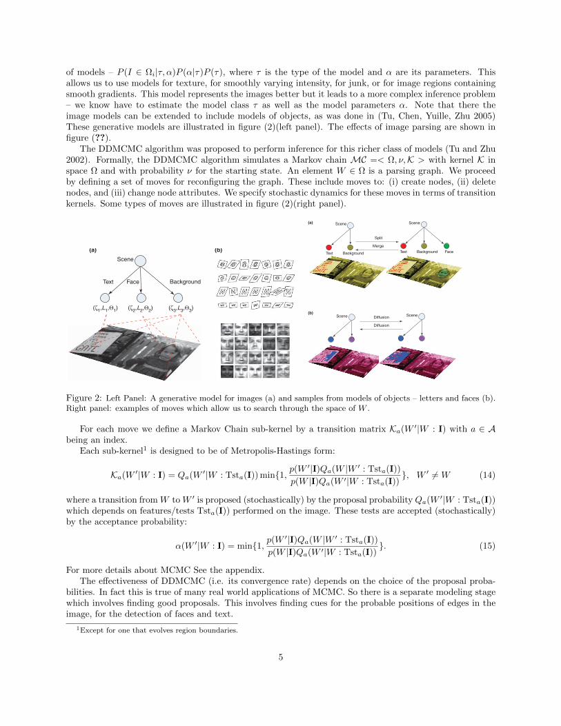
of models – P (I ∈ Ωi|τ, α)P (α|τ)P (τ), where τ is the type of the model and α are its parameters. Thisallows us to use models for texture, for smoothly varying intensity, for junk, or for image regions containingsmooth gradients. This model represents the images better but it leads to a more complex inference problem– we know have to estimate the model class τ as well as the model parameters α. Note that there theimage models can be extended to include models of objects, as was done in (Tu, Chen, Yuille, Zhu 2005)These generative models are illustrated in figure (2)(left panel). The effects of image parsing are shown infigure (??).

The DDMCMC algorithm was proposed to perform inference for this richer class of models (Tu and Zhu2002). Formally, the DDMCMC algorithm simulates a Markov chain MC =< Ω, ν,K > with kernel K inspace Ω and with probability ν for the starting state. An element W ∈ Ω is a parsing graph. We proceedby defining a set of moves for reconfiguring the graph. These include moves to: (i) create nodes, (ii) deletenodes, and (iii) change node attributes. We specify stochastic dynamics for these moves in terms of transitionkernels. Some types of moves are illustrated in figure (2)(right panel).

Text BackgroundFace

(ζ3,L3,Θ3)(ζ2,L2,Θ2)(ζ1,L1,Θ1)

Scene

(a) (b)

Scene Scene

Text Background

Merge

Split

Text FaceBackground

SceneScene

Diffusion

Diffusion

(a)

(b)

Figure 2: Left Panel: A generative model for images (a) and samples from models of objects – letters and faces (b).Right panel: examples of moves which allow us to search through the space of W .

For each move we define a Markov Chain sub-kernel by a transition matrix Ka(W ′|W : I) with a ∈ Abeing an index.

Each sub-kernel1 is designed to be of Metropolis-Hastings form:

Ka(W ′|W : I) = Qa(W ′|W : Tsta(I)) min1, p(W′|I)Qa(W |W ′ : Tsta(I))

p(W |I)Qa(W ′|W : Tsta(I)), W ′ 6= W (14)

where a transition from W to W ′ is proposed (stochastically) by the proposal probability Qa(W ′|W : Tsta(I))which depends on features/tests Tsta(I)) performed on the image. These tests are accepted (stochastically)by the acceptance probability:

α(W ′|W : I) = min1, p(W′|I)Qa(W |W ′ : Tsta(I))

p(W |I)Qa(W ′|W : Tsta(I)). (15)

For more details about MCMC See the appendix.The effectiveness of DDMCMC (i.e. its convergence rate) depends on the choice of the proposal proba-

bilities. In fact this is true of many real world applications of MCMC. So there is a separate modeling stagewhich involves finding good proposals. This involves finding cues for the probable positions of edges in theimage, for the detection of faces and text.

1Except for one that evolves region boundaries.

5

/a. Input image b. Segmentation c. Synthesized image d. Manual segmentation

(a)

(b)

Figure 3: Left Panel: the need for object models to obtain good segmentation. The input image (a),segmentation by a model (Tu znd Zhu) which does not use models of objects, (c) the image re-sampled fromthe Tu and Zhu model, (d) the groundtruth segmentation. Right Panel: the effect of using object models.The input image (upper left) and the proposals for faces and text (upper right). The segmentation (lowerleft), the text and faces detected (lower center), and the re-sampled image (lower right).

4.1 Generative Models

The number K of intermediate nodes is a random variable, and each node i = 1, ...,K has a set of attributes(Li, ζi,Θi) defined as follows. Li is the shape descriptor and determines the region Ri = R(Li) of the imagepixels covered by the visual pattern of the intermediate node. Conceptually, the pixels within Ri are childnodes of the intermediate node i. (Regions may contain holes, in which case the shape descriptor will haveinternal and external boundaries). The remaining attribute variables (ζi,Θi) specify the probability modelsp(IR(Li)|ζi, Li,Θi) for generating the sub-image IR(Li) in region R(Li). The variables ζi ∈ 1, ..., 66 indicatethe visual pattern type (3 types of generic visual patterns, 1 face pattern, and 62 text character patterns),and Θi denotes the model parameters for the corresponding visual pattern (details are given in the followingsubsections). The complete scene description can be summarized by:

W = (K, (ζi, Li,Θi) : i = 1, 2, ...,K).

The shape descriptors Li : i = 1, ...,K are required to be consistent so that each pixel in the image isa child of one, and only one, of the intermediate nodes. The shape descriptors must provide a partition ofthe image lattice Λ = (m,n) : 1 ≤ m ≤ Height(I), 1 ≤ n ≤Width(I) and hence satisfy the condition

Λ = ∪Ki=1R(Li), R(Li) ∩R(Lj) = ∅, ∀i 6= j.

The generation process from the scene description W to I is governed by the likelihood function:

p(I|W ) =

K∏i=1

p(IR(Li)|ζi, Li,Θi).

The prior probability p(W ) is defined by

p(W ) = p(K)

K∏i=1

p(Li)p(ζi|Li)p(Θi|ζi).

In our Bayesian formulation, parsing the image corresponds to computing the W ∗ that maximizes aposteriori probability over Ω, the solution space of W ,

W ∗ = arg maxW∈Ω

p(W |I) = arg maxW∈Ω

p(I|W )p(W ). (16)

It remains to specify the prior p(W ) and the likelihood function p(I|W ). We set the prior terms p(K)and p(Θi|ζi) to be uniform probabilities. The term p(ζi|Li) is used to penalize high model complexity.

6

4.2 Generative intensity models

We use four families of generative intensity models for describing intensity patterns of (approximately)constant intensity, clutter/texture, shading, and faces (a fifth model for letters is omitted for reasons ofspace). The first three are similar to those defined in (Tu and Zhu 2002).1. Constant intensity model ζ = 1:.

This assumes that pixel intensities in a region R are subject to independently and identically distributed(iid) Gaussian distribution,

p1(IR(L)|ζ = 1, L,Θ) =∏

v∈R(L)

G(Iv − µ;σ2), Θ = (µ, σ)

2. Clutter/texture model ζ = 2:.This is a non-parametric intensity histogram h() discretized to take G values (i.e. is expressed as a vector

(h1, h2, ..., hG)). Let nj be the number of pixels in R(L) with intensity value j.

p2(IR(L)|ζ = 2, L,Θ) =∏

v∈R(L)

h(Iv) =

G∏j=1

hnjj , Θ = (h1, h2, ..., hG).

3. Shading model ζ = 3 and ζ = 5, ..., 66:.This family of models are used to describe generic shading patterns, and text characters. We use a

quadratic formJ(x, y; Θ) = ax2 + bxy + cy2 + dx+ ey + f,

with parameters Θ = (a, b, c, d, e, f, σ). Therefore, the generative model for pixel (x, y) is

p3(IR(L)|ζ ∈ 3, (5, ..., 66), L,Θ) =∏

v∈R(L)

G(Iv − Jv;σ2), Θ = (a, b, c, d, e, f, σ).

4. The PCA face model ζ = 4:.The generative model for faces is simpler and uses Principal Component Analysis (PCA) to obtain

representations of the faces in terms of principal components Bi and covariances Σ. Lower level features,also modeled by PCA, can be added. Figure ?? shows some faces sampled from the PCA model.

p4(IR(L)|ζ = 4, L,Θ) = G(IR(L) −∑i

λiBi; Σ), Θ = (λ1, .., λn,Σ).

5. Models of Text ζ = 5:. Conceptually straightfroward. Too complex to include.

4.3 Proposal Probabilities

The proposal probabilities q(wj |Tstj(I)) make proposals for the elementary components wj of W . Forcomputational efficiency, these probabilities are based only on a small number of simple tests Tstj(I). Thecues are of the following forms:

1. Edge Cues. These cues are based on edge detectors. They are used to give proposals for regionboundaries (i.e. the shape descriptor attributes of the nodes). Specifically, we run the Canny detector atthree scales followed by edge linking to give partitions of the image lattice. This gives a finite list of candidatepartitions which are assigned weights, see section (5.2.3). The probability is represented by this weightedlist of particles (similar to particle filtering).

2. Binarization Cues. These cues are computed using a variant of Niblack’s algorithm. They areused to propose boundaries for text characters (i.e. shape descriptors for text nodes), and will be used inconjunction with proposals for text detection. Like edge cues, the algorithm is run at different parameterssettings and represents the discriminative probability by a weighted list of particles indicating candidateboundary locations.

7

3. Face Region Cues. These cues are learnt by a variant of AdaBoost which outputs probabilities(Hastie, Tibishani, Friedman). They propose the presence of faces in sub-regions of the image. These cuesare combined with edge detection to propose the localization of faces in an image.

4. Text Region Cues. These cues are also learnt by a probabilistic version of AdaBoost. The algorithmis applied to image windows (at a range of scales). It outputs a discriminative probability for the presenceof text in each window. Text region cues are combined with binarization to propose boundaries for textcharacters.

5. Shape Affinity Cues. These act on shape boundaries, produced by binarization, to propose textcharacters. They use shape context cues and information features to propose matches between the shapeboundaries and the deformable template models of text characters.

6. Region Affinity Cues. These are used to estimate whether two regions Ri, Rj are likely to havebeen generated by the same visual pattern family and model parameters. They use an affinity similaritymeasure of the intensity properties IRi , IRj .

7. Model Parameter and Visual Pattern Family cues. These are used to propose model parametersand visual pattern family identity. They are based on clustering algorithms, such as mean-shift. .

In our current implementation, we conduct all the bottom-up tests Tstj(I), j = 1, 2, ...,K at an earlystage for all the probability models qj(wj |Tstj(I)), and they are then combined to form composite testsTsta(I) for each subkernel Ka in equations (14,15).

4.4 Control Structure of the Algorithm

The control strategy used by our image parser explores the space of parsing graphs by a Markov Chain MonteCarlo sampling algorithm. This algorithm uses a transition kernel K which is composed of sub-kernels Kacorresponding to different ways to reconfigure the parsing graph. These sub-kernels come in reversible pairs2

(e.g. birth and death) and are designed so that the target probability distribution of the kernel is thegenerative posterior p(W |I). At each time step, a sub-kernel is selected stochastically. The sub-kernelsuse the Metropolis-Hasting sampling algorithm, see equation (14), which proceeds in two stages. First, itproposes a reconfiguration of the graph by sampling from a proposal probability. Then it accepts or rejectsthis reconfiguration by sampling the acceptance probability.

To summarize, we outline the control strategy of the algorithm below. At each time step, it specifies(stochastically) which move to select (i.e. which sub-kernel), where to apply it in the graph, and whetherto accept the move. The probability to select moves ρ(a : I) was first set to be independent of I, but wegot better performance by adapting it using discriminative cues to estimate the number of faces and textcharacters in the image (see details below). The choice of where to apply the move is specified (stochastically)by the sub-kernel. For some sub-kernels it is selected randomly and for others is chosen based on a fitnessfactor (see details in section (5)), which measures how well the current model fits the image data.

2Except for the boundary evolution sub-kernel which will be described separately, see Section 5.1.

8

The basic control strategy of the image parsing algorithm

1. Initialize W (e.g. by dividing the image into four regions), setting their shape descriptors,and assigning the remaining node attributes at random.

2. Set the temperature to be Tinit.

3. Select the type a of move by sampling from a probability ρ(a), with ρ(1) = 0.2 for faces,ρ(2) = 0.2 for text, ρ(3) = 0.4 for splitting and merging, ρ(4) = 0.15 for switching regionmodel (type or model parameters), and ρ(5) = 0.05 for boundary evolution. This was modifiedslightly adaptively, see caption and text.

4. If the selected move is boundary evolution, then select adjacent regions (nodes) at randomand apply stochastic steepest descent, see section (5.1).

5. If the jump moves are selected, then a new solution W ′ is randomly sampled as follows:

− For the birth or death of a face, see section (5.2.2), we propose to create or delete aface. This includes a proposal for where in the image to do this.

− For the birth of death of text, see section (5.2.1), we propose to create a text characteror delete an existing one. This includes a proposal for where to do this.

− For region splitting, see section (5.2.3), a region (node) is randomly chosen biased byits fitness factor. There are proposals for where to split it and for the attributes of theresulting two nodes.

− For region merging, see section (5.2.3), two neighboring regions (nodes) are selectedbased on a proposal probability. There are proposals for the attributes of the resultingnode.

− For switching, see section (5.2.4), a region is selected randomly according to its fitnessfactor and a new region type and/or model parameters is proposed.

• The full proposal probabilities, Q(W |W : I) and Q(W ′|W : I) are computed.

• The Metropolis-Hastings algorithm, equation (14), is applied to accept or reject theproposed move.

6. Reduce the temperature T = 1 + Tinit × exp(−t× c|R|), where t is the current iteration step,c is a constant and |R| is the size of the image.

7. Repeat the above steps and until the convergence criterion is satisfied (by reaching the max-imum number of allowed steps or by lack of decrease of the negative log posterior).

5 The Markov Chain kernels

This section gives a detailed discussion of the individual Markov Chain kernel, their proposal probabilities,and their fitness factors.

5.1 Boundary Evolution

These moves evolve the positions of the region boundaries but preserve the graph structure. They areimplemented by a stochastic partial differential equation (Langevin equation) driven by Brownian noise andcan be derived from a Markov Chain. The deterministic component of the PDE is obtained by performingsteepest descent on the negative log-posterior, as derived in (Zhu and Yuille 1996).

We illustrate the approach by deriving the deterministic component of the PDE for the evolution of theboundary between a letter Tj and a generic visual pattern region Ri. The boundary will be expressed interms of the control points Sm of the shape descriptor of the letter. Let v denote a point on the boundary,i.e. v(s) = (x(s), y(s)) on Γ(s) = ∂Ri ∩ ∂Rj . The deterministic part of the evolution equation is obtainedby taking the derivative of the negative log-posterior − log p(W |I) with respect to the control points.

More precisely, the relevant parts of the negative log-posterior, see equation (16,4.1) are given by E(Ri)and E(Tj) where:

E(Ri) =

∫ ∫Ri

− log p(I(x, y)|θζi)dxdy + γ|Ri|α + λ|∂Ri|.

9

and

E(Tj) =

∫ ∫Lj

log p(I(x, y)|θζj )dxdy + γ|R(Lj)|α − log p(Lj).

Differentiating E(Ri) + E(Tj) with respect to the control points Sm yields the evolution PDE:

dSmdt

= −δE(Ri)

δSm− δE(Tj)

δSm

=

∫[−δE(Ri)

δv− δE(Tj)

δv]

1

|J(s)|ds

=

∫n(v)[log

p(I(v); θζi)

p(I(v); θζj )+ αγ(

1

|Dj |1−α− 1

|Di|1−α)− λκ+D(GSj (s)||GT (s))]

1

|J(s)|ds,

where J(s) is the Jacobian matrix for the spline function. (Recall that α = 0.9 in the implementation).

The log-likelihood ratio term logp(I(v);θζi )

p(I(v);θζj ) implements the competition between the letter and the generic

region models for ownership of the boundary pixels.

5.2 Markov chain sub-kernels

Changes in the graph structure are realized by Markov chain jumps implemented by four different sub-kernels.

5.2.1 Sub-kernel I: birth and death of text

This pair of jumps is used to create or delete text characters. We start with a parse graph W and transitioninto parse graph W ′ by creating a character. Conversely, we transition from W ′ back to W by deleting acharacter.

The proposals for creating and deleting text characters are designed to approximate the terms in equa-tion (??). We obtain a list of candidate text character shapes by using AdaBoost to detect text regionsfollowed by binarization to detect candidate text character boundaries within text regions. This list is rep-resented by a set of particles which are weighted by the similarity to the deformable templates for textcharacters (see below):

S1r(W ) = (z(µ)1r , ω

(µ)1r ) : µ = 1, 2, ..., N1r.

Similarly, we specify another set of weighted particles for removing text characters:

S1l(W′) = (z

(ν)1l , ω

(ν)1l ) : ν = 1, 2, ..., N1l.

z(µ)1r and z(ν)

1l represent the possible (discretized) shape positions and text character deformable templates

for creating or removing text, and ω(µ)1r and ω(ν)

1l are their corresponding weights. The particles are thenused to compute proposal probabilities

Q1r(W′|W : I) =

ω1r(W′)∑N1r

µ=1 ω(µ)1r

, Q1l(W |W ′, I) =ω1l(W )∑N1l

ν=1 ω(ν)1l

.

The weights ω(µ)1r and ω

(ν)1l for creating new text characters are specified by shape affinity measures, such

as shape contexts. For deleting text characters we calculate ω(ν)1l directly from the likelihood and prior on

the text character. Ideally these weights will approximate the ratios p(W ′|I)p(W |I) and p(W |I)

p(W ′|I) .

5.2.2 Sub-kernel II: birth and death of face

The sub-kernel for the birth and death of faces is very similar to the sub-kernel of birth and death of text.We use AdaBoost to detect candidate faces. Face boundaries are obtained directly from using edge detectionto give candidate face boundaries. The proposal probabilities are computed similarly to those for sub-kernelI.

10

5.2.3 Sub-kernel III: splitting and merging regions

This pair of jumps is used to create or delete nodes by splitting and merging regions (nodes). We start witha parse graph W and transition into parse graph W ′ by splitting node i into nodes j and k. Conversely, wetransition back to W by merging nodes j and k into node i. The selection of which region i to split is basedon a robust function on p(IRi |ζi, Li,Θi) (i.e. the worse the model for region Ri fits the data, the more likelywe are to split it). For merging, we use a region affinity measure and propose merges between regions whichhave high affinity.

Formally, we define W,W ′:

W = (K, (ζk, Lk,Θk),W−) W ′ = (K + 1, (ζi, Li,Θi), (ζj , Lj ,Θj),W−)

where W− denotes the attributes of the remaining K − 1 nodes in the graph.We obtain proposals by seeking approximations to equation (??) as follows.We first obtain three edge maps. These are given by Canny edge detectors at different scales. We use

these edge maps to create a list of particles for splitting S3r(W ). A list of particles for merging is denotedby S3l(W

′).

S3r(W ) = (z(µ)3r , ω

(µ)3r ) : µ = 1, 2, ..., N3r., S3l(W

′) = (z(ν)3l , ω

(ν)3l ) : ν = 1, 2, ..., N3l.

where z(µ)3r and z(ν)

3l represent the possible (discretized) positions for splitting and merging, and theirweights ω3r, ω3l will be defined shortly. In other words, we can only split a region i into regions j andk along a contour zµ3r (i.e. zµ3r forms the new boundary). Similarly we can only merge regions j and k intoregion i by deleting a boundary contour zµ3l.

We now define the weights ω3r, ω3l. These weights will be used to determine probabilities for thesplits and merges by:

Q3r(W′|W : I) =

ω3r(W′)∑N3r

µ=1 ω(µ)3r

, Q3l(W |W ′ : I) =ω3l(W )∑N3l

ν=1 ω(ν)3l

.

Again, we would like ωµ3r and ων3l to approximate the ratios p(W |I)p(W ′|I) and p(W ′|I)

p(W |I) respectively. p(W ′|I)p(W |I) is

given by:

p(W ′|I)

p(W |I)=p(IRi |ζi, Li,Θi)p(IRj |ζj , Lj ,Θj)

p(IRk |ζk, Lk,Θk)· p(ζi, Li,Θi)p(ζj , Lj ,Θj)

p(ζk, Lk,Θk)· p(K + 1)

p(K)

This is expensive to compute, so we approximate p(W ′|I)p(W |I) and p(W |I)

p(W ′|I) by:

ω(µ)3r =

q(Ri, Rj)

p(IRk |ζk, Lk,Θk)· [q(Li)q(ζi,Θi)][q(Lj)q(ζj ,Θj)]

p(ζk, Lk,Θk). (17)

ω(ν)3l =

q(Ri, Rj)

p(IRi |ζi, Li,Θi)p(IRj |ζj , Lj ,Θj)· q(Lk)q(ζk,Θk)

p(ζi, Li,Θi)p(ζj , Lj ,Θj), (18)

Where q(Ri, Rj) is an affinity measure of the similarity of the two regions Ri and Rj (it is a weighted sumof the intensity difference |Ii− Ij | and the chi-squared difference between the intensity histograms), q(Li) isgiven by the priors on the shape descriptors, and q(ζi,Θi) is obtained by clustering in parameter space.

5.2.4 Jump II: Switching Node Attributes

These moves switch the attributes of a node i. This involves changing the region type ζi and the modelparameters Θi.

The move transitions between two states:

W = ((ζi, Li,Θi),W−) W ′ = ((ζ ′i, L′i,Θ′i),W−)

11

The proposal should approximate:

p(W ′|I)

p(W |I)=p(IRi |ζ ′i, L′i,Θ′i)p(ζ ′i, L′i,Θ′i)p(IRi |ζi, Li,Θi)p(ζi, Li,Θi)

.

We approximate this by a weight ω(µ)4 given by

ω(µ)4 =

q(L′i)q(ζ′i,Θ′i)

p(IRi |ζi, Li,Θi)p(ζi, Li,Θi),

where q(L′i)q(ζ′i,Θ′i) are the same functions used in the split and merge moves. The proposal probability is

the weight normalized in the candidate set, Q4(W ′|W : I) = ω4(W ′)∑N4µ=1 ω

(µ)4

.

Appendix: Markov Chain kernels and sub-kernels

For each move we define a Markov Chain sub-kernel by a transition matrix Ka(W ′|W : I) with a ∈ Abeing an index. This represents the probability that the system makes a transition from state W to stateW ′ when sub-kernel a is applied (i.e.

∑W ′ Ka(W ′|W : I) = 1, ∀ W ). Kernels which alter the graph

structure are grouped into reversible pairs. For example, the sub-kernel for node creation Ka,r(W ′|W : I) ispaired with the sub-kernel for node deletion Ka,l(W ′|W : I). This can be combined into a paired sub-kernelKa = ρarKa,r(W ′|W : I) + ρalKa,l(W ′|W : I) (ρar + ρal = 1). This pairing ensures that Ka(W ′|W : I) = 0if, and only if, Ka(W |W ′ : I) = 0 for all states W,W ′ ∈ Ω. The sub-kernels (after pairing) are constructedto obey the detailed balance condition:

p(W |I)Ka(W ′|W : I) = p(W ′|I)Ka(W |W ′ : I). (19)

The full transition kernel is expressed as:

K(W ′|W : I) =∑a

ρ(a : I)Ka(W ′|W : I),∑a

ρ(a : I) = 1, ρ(a : I) > 0. (20)

To implement this kernel, at each time step the algorithm selects the choice of move with probabilityρ(a : I) for move a, and then uses kernel Ka(W ′|W ; I) to select the transition from state W to state W ′.Note that both probabilities ρ(a : I) and Ka(W ′|W ; I) depend on the input image I.

The full kernel obeys detailed balance, equation (19), because all the sub-kernels do. It will also beergodic, provided the set of moves is sufficient (i.e. so that we can transition between any two statesW,W ′ ∈ Ω using these moves). These two conditions ensure that p(W |I) is the invariant (target) probabilityof the Markov Chain.

Applying the kernel Ka(t) updates the Markov chain state probability µt(W ) at step t to µt+1(W ′) att+ 1:

µt+1(W ′) =∑W

Ka(t)(W′|W : I)µt(W ). (21)

In summary, the DDMCMC image parser simulates a Markov chain MC with a unique invariant proba-bility p(W |I). At time t, the Markov chain state (i.e. the parse graph) W follows a probability µt which isthe product of the sub-kernels selected up to time t,

W ∼ µt(W ) = ν(Wo) · [Ka(1) Ka(2) · · · Ka(t)](Wo,W ) −→ p(W |I). (22)

where a(t) indexes the sub-kernel selected at time t. As the time t increases, µt(W ) approaches the pos-terior p(W |I) monotonically at a geometric rate independent of the starting configuration. The followingconvergence theorem is useful for image parsing because it helps quantify the effectiveness of the differentsub-kernels.

12

Theorem 1 The Kullback-Leibler divergence between the posterior p(W |I) and the Markov chain state prob-ability decreases monotonically when a sub-kernel Ka(t),∀ a(t) ∈ A is applied,

KL(p(W |I) ||µt(W ))−KL(p(W |I) ||µt+1(W )) ≥ 0 (23)

The decrease of KL-divergence is strictly positive and is equal to zero only after the Markov chain becomesstationary, i.e. µ = p.

The theorem is related to the second law of thermodynamics, and its proof makes use of the detailedbalance equation (19). This KL divergence gives a measure of the “power” of each sub-kernel Ka(t) andso it suggests an efficient mechanism for selecting the sub-kernels at each time step, see Section (??). Bycontrast, classic convergence analysis shows that the convergence of the Markov Chain is exponentially fast,but does not give measures of power of sub-kernels.

Proof. For notational simplicity, we ignore the dependencies on the kernels and probabilities on the inputimage I.

Let µt(Wt) be the state probability at time step t. After applying a sub-kernel Ka(Wt+1|Wt), its statebecomes Wt+1 with probability:

µt+1(Wt+1) =∑Wt

µt(Wt)Ka(Wt+1|Wt). (24)

The joint probability µ(Wt,Wt+1) for Wt and Wt+1 can be expressed in two ways as:

µ(Wt,Wt+1) = µt(Wt)Ka(Wt+1|Wt) = µt+1(Wt+1)pMC(Wt|Wt+1), (25)

where pMC(Wt|Wt+1) is the “posterior” probability for state Wt at time step t conditioned on state Wt+1

at time step t+ 1.This joint probability µ(Wt,Wt+1) can be compared to the joint probability p(Wt,Wt+1) at equilibrium

(i.e. when µt(Wt) = P (Wt)). We can also express p(Wt,Wt+1) in two ways:

p(Wt,Wt+1) = p(Wt)Ka(Wt+1|Wt) = p(Wt+1)Ka(Wt+1,Wt), (26)

where the second equality is obtained using the detailed balance condition on Ka.We calculate the Kullback-Leibler (K-L) divergence between the joint probabilities P (Wt,Wt+1) and

µ(Wt,Wt+1) in two ways using the first and second equalities in equations (25,26). We obtain two expressions(1 & 2) for the K-L divergence:

KL(p(Wt,Wt+1) ||µ(Wt,Wt+1)) =∑Wt+1

∑Wt

p(Wt,Wt+1) logp(Wt,Wt+1)

µ(Wt,Wt+1)

1=

∑Wt

p(Wt)∑Wt+1

Ka(Wt+1|Wt)) logp(Wt) · Ka(Wt+1|Wt)

µt(Wt)Ka(Wt+1|Wt)

= KL(p(W ) ||µt(W )) (27)

2=

∑Wt+1

∑Wt

Ka(Wt|Wt+1))p(Wt+1) logp(Wt+1)Ka(Wt|Wt+1)

µt+1(Wt+1)pMC(Wt|Wt+1)

= KL(p(Wt+1) ||µt+1(W )) + Ep(Wt+1)[KL(Ka(Wt|Wt+1)||pMC(Wt|Wt+1))] (28)

We equate the two alternatives expressions for the KL divergence, using equations (27) and (28), andobtain

KL(p(W ) ||µt(W ))−KL(p(W ) ||µt+1(W )) = Ep(Wt+1)[KL(Ka(t)(Wt|Wt+1)||pMC(Wt|Wt+1))]

This proves that the K-L divergence decreases monotonically. The decrease is zero only whenKa(t)(Wt|Wt+1) =pMC(Wt|Wt+1) (because KL(p||µ) ≥ 0 with equality only when p = µ). This occurs if and only ifµt(W ) = p(W ) (using the definition of pMC(Wt|Wt+1), given in equation (25), and the detailed balanceconditions for Ka(t)(Wt|Wt+1)). [End of Proof].

13