lecture 11: benders decomposition - chalmers€¦ · benders decomposition for mixed-integer...

Lecture 11: Benders decomposition

Michael Patriksson

28 September 2009

Michael Patriksson Benders decomposition

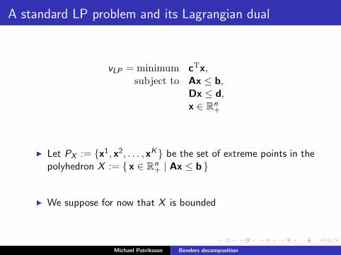
A standard LP problem and its Lagrangian dual

vLP = minimum cTx,

subject to Ax ≤ b,

Dx ≤ d,

x ∈ Rn+

�Let PX := {x1, x2, . . . , xK} be the set of extreme points in thepolyhedron X := { x ∈ R

n+ | Ax ≤ b }

�We suppose for now that X is bounded


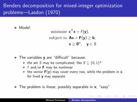
Benders decomposition for mixed-integer optimization

problems—Lasdon (1970)

�Model:

minimize cTx + f (y),

subject to Ax + F(y) ≥ b,

x ≥ 0n, y ∈ S

�The variables y are “difficult” because:

� the set S may be complicated, like S ⊆ {0, 1}p

�f and/or F may be nonlinear

� the vector F(y) may cover every row, while the problem in x

for fixed y may separate

�The problem is linear, possibly separable in x; “easy”


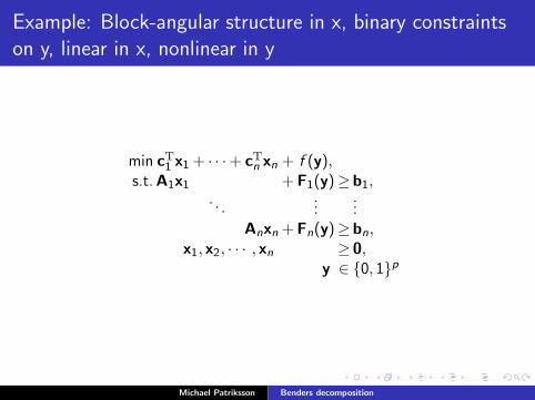
Example: Block-angular structure in x, binary constraints

on y, linear in x, nonlinear in y

min cT

1 x1 + · · ·+ cTn xn + f (y),

s.t. A1x1 + F1(y)≥b1,. . .

......

Anxn +Fn(y)≥bn,

x1, x2, · · · , xn ≥ 0,

y ∈ {0, 1}p


Applications

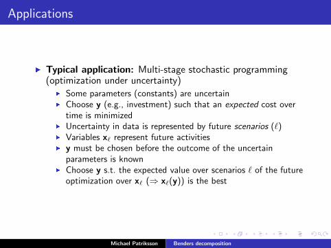
�Typical application: Multi-stage stochastic programming(optimization under uncertainty)

� Some parameters (constants) are uncertain� Choose y (e.g., investment) such that an expected cost over

time is minimized� Uncertainty in data is represented by future scenarios (`)� Variables x` represent future activities�

y must be chosen before the outcome of the uncertainparameters is known

� Choose y s.t. the expected value over scenarios ` of the futureoptimization over x` (⇒ x`(y)) is the best


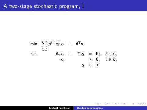
A two-stage stochastic program, I

min∑

`∈L

p` · cT

` x` + dTy,

s.t. A`x` + T`y = b`, ` ∈ L,

x` ≥ 0, ` ∈ L,

y ∈ Y


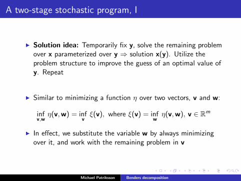
A two-stage stochastic program, I

�Solution idea: Temporarily fix y, solve the remaining problemover x parameterized over y ⇒ solution x(y). Utilize theproblem structure to improve the guess of an optimal value ofy. Repeat

�Similar to minimizing a function η over two vectors, v and w:

infv,w

η(v,w) = infv

ξ(v), where ξ(v) = infw

η(v,w), v ∈ Rm

�In effect, we substitute the variable w by always minimizingover it, and work with the remaining problem in v


Benders decomposition

�Benders decomposition: construct an approximation of thisproblem over v by utilizing LP duality

�If the problem over y is also linear

⇒ cutting plane methods from above

�Benders decomposition is more general:Solves problems with positive duality gaps!

�Benders decomposition does not rely on the existence ofoptimal Lagrange multipliers and strong duality


The Benders sub- and master problems, I

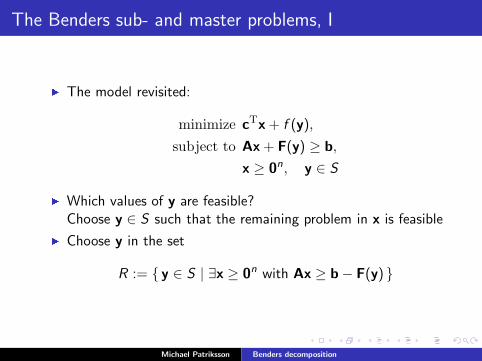
�The model revisited:



x ≥ 0n, y ∈ S

�Which values of y are feasible?Choose y ∈ S such that the remaining problem in x is feasible

�Choose y in the set

R := { y ∈ S | ∃x ≥ 0n with Ax ≥ b − F(y) }


The Benders sub- and master problems, II

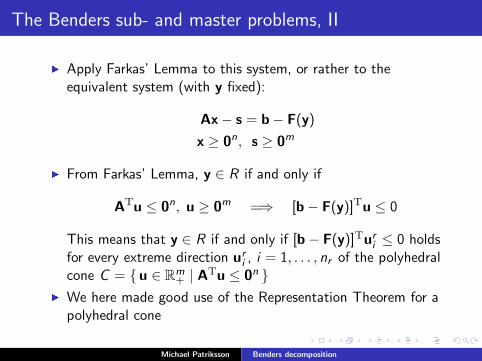
�Apply Farkas’ Lemma to this system, or rather to theequivalent system (with y fixed):

Ax − s = b − F(y)

x ≥ 0n, s ≥ 0m

�From Farkas’ Lemma, y ∈ R if and only if

ATu ≤ 0n, u ≥ 0m =⇒ [b − F(y)]Tu ≤ 0

This means that y ∈ R if and only if [b − F(y)]Turi ≤ 0 holds

for every extreme direction uri , i = 1, . . . , nr of the polyhedral

cone C = {u ∈ Rm+ | ATu ≤ 0n }

�We here made good use of the Representation Theorem for apolyhedral cone


The Benders sub- and master problems, III

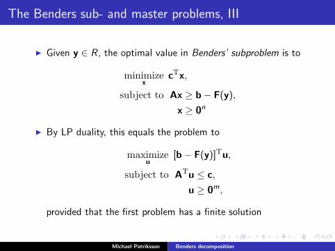
�Given y ∈ R , the optimal value in Benders’ subproblem is to

minimizex

cTx,

subject to Ax ≥ b − F(y),

x ≥ 0n

�By LP duality, this equals the problem to

maximizeu

[b − F(y)]Tu,

subject to ATu ≤ c,

u ≥ 0m,

provided that the first problem has a finite solution


The Benders sub- and master problems, IV

�We prefer the dual formulation, since its constraints do notdepend on y

�Moreover, the extreme directions of its feasible set are givenby the vectors ur

i , i = 1, . . . , nr , discussed above

�Let u

pi , i = 1, . . . , np , denote the extreme points of this set

�This completes the subproblem

�Let’s now study the restricted master problem (RMP) ofBenders’ algorithm


The Benders sub- and master problems, V

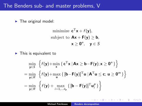
�The original model:



x ≥ 0n, y ∈ S

�This is equivalent to

miny∈S

{

f (y)+minx

{ cTx |Ax ≥ b−F(y); x ≥ 0n }}

= miny∈R

{

f (y)+maxu

{ [b−F(y)]Tu |ATu ≤ c; u ≥ 0m }}

= miny∈R

{

f (y) + maxi=1,...np

{ [b − F(y)]Tupi }

}


The Benders sub- and master problems, VI

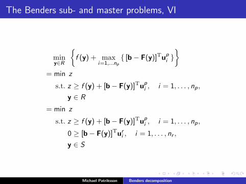
miny∈R

{

f (y) + maxi=1,...np

{ [b − F(y)]Tupi }

}

= min z

s.t. z ≥ f (y) + [b − F(y)]Tupi , i = 1, . . . , np ,

y ∈ R

= min z

s.t. z ≥ f (y) + [b − F(y)]Tupi , i = 1, . . . , np ,

0 ≥ [b − F(y)]Turi , i = 1, . . . , nr ,

y ∈ S


The Benders sub- and master problems, VII

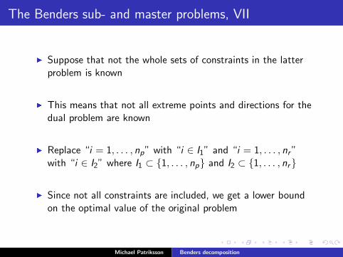
�Suppose that not the whole sets of constraints in the latterproblem is known

�This means that not all extreme points and directions for thedual problem are known

�Replace “i = 1, . . . , np” with “i ∈ I1” and “i = 1, . . . , nr”with “i ∈ I2” where I1 ⊂ {1, . . . , np} and I2 ⊂ {1, . . . , nr}

�Since not all constraints are included, we get a lower boundon the optimal value of the original problem


The Benders sub- and master problems, VIII

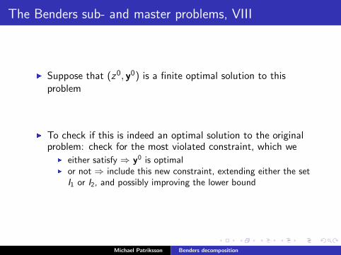
�Suppose that (z0, y0) is a finite optimal solution to thisproblem

�To check if this is indeed an optimal solution to the originalproblem: check for the most violated constraint, which we

� either satisfy ⇒ y0 is optimal� or not ⇒ include this new constraint, extending either the set

I1 or I2, and possibly improving the lower bound


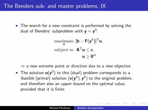
The Benders sub- and master problems, IX

�The search for a new constraint is performed by solving thedual of Benders’ subproblem with y = y0:

maximumu

[b − F(y0)]Tu,

subject to ATu ≤ c,

u ≥ 0m

⇒ a new extreme point or direction due to a new objective�

The solution u(y0) to this (dual) problem corresponds to afeasible (primal) solution (x(y0), y0) to the original problem,and therefore also an upper bound on the optimal value,provided that it is finite


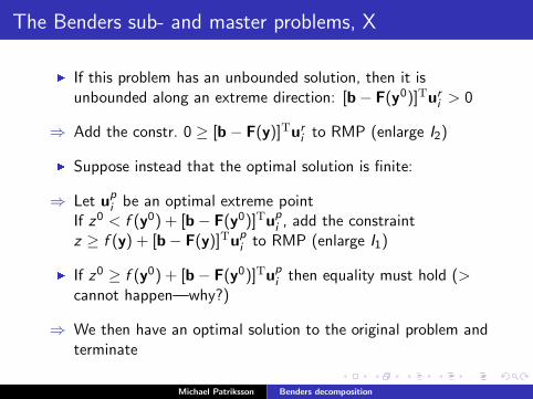
The Benders sub- and master problems, X

�If this problem has an unbounded solution, then it isunbounded along an extreme direction: [b − F(y0)]Tur

i > 0

⇒ Add the constr. 0 ≥ [b − F(y)]Turi to RMP (enlarge I2)

�Suppose instead that the optimal solution is finite:

⇒ Let upi be an optimal extreme point

If z0 < f (y0) + [b − F(y0)]Tupi , add the constraint

z ≥ f (y) + [b − F(y)]Tupi to RMP (enlarge I1)

�If z0 ≥ f (y0) + [b − F(y0)]Tu

pi then equality must hold (>

cannot happen—why?)

⇒ We then have an optimal solution to the original problem andterminate


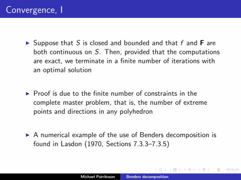
Convergence, I

�Suppose that S is closed and bounded and that f and F areboth continuous on S . Then, provided that the computationsare exact, we terminate in a finite number of iterations withan optimal solution

�Proof is due to the finite number of constraints in thecomplete master problem, that is, the number of extremepoints and directions in any polyhedron

�A numerical example of the use of Benders decomposition isfound in Lasdon (1970, Sections 7.3.3–7.3.5)


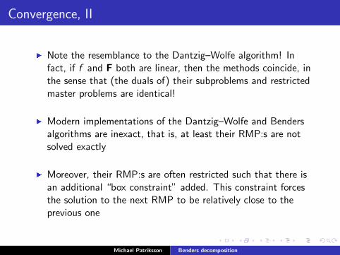
Convergence, II

�Note the resemblance to the Dantzig–Wolfe algorithm! Infact, if f and F both are linear, then the methods coincide, inthe sense that (the duals of) their subproblems and restrictedmaster problems are identical!

�Modern implementations of the Dantzig–Wolfe and Bendersalgorithms are inexact, that is, at least their RMP:s are notsolved exactly

�Moreover, their RMP:s are often restricted such that there isan additional “box constraint” added. This constraint forcesthe solution to the next RMP to be relatively close to theprevious one


Convergence, III

�The effect is that of a stabilization; otherwise, there is a riskthat the sequence of solutions to the RMP:s “jump about,”and convergence becomes slow as the optimal solution isapproached

�This was observed quite early on with the Dantzig–Wolfealgorithm, which even can be enriched with non-linear“penalty” terms in the RMP to further stabilize convergence

�In any case, convergence holds also under these modifications,except perhaps for the finiteness


lecture 11: benders decomposition - chalmers€¦ · benders decomposition for mixed-integer...

Documents