lections №5 using statistica fot the statistical hypothesis testing

LectionsLections № №55

Using STATISTICA fot the Statistical Hypothesis

Testing

Main QuestionsMain Questions

Descriptive statistics.Statistical hypothesis testing.Regression Analysis BasicsThe STATISTICA usage example.

1.Descriptive statistics1.Descriptive statistics StatisticStatistic - - Measure of a sample characteristic.Measure of a sample characteristic. PopulationPopulation - Contains all members of a group. SampleSample - A subset of a population. Interval DataInterval Data - Objects classified by type or characteristic,

with logical order and equal differences between levels of data.

Ordinal DataOrdinal Data - Objects classified by type or characteristic with some logical order.

VariableVariable - A characteristic that can form different values from one observation to another.

Independent VariableIndependent Variable - A measure that can take on different values which are subject to manipulation by the researcher.

Response VariableResponse Variable - The measure not controlled in an experiment. Commonly known as the dependent variable.

1.1.1.1.Descriptive statisticsDescriptive statisticsFor interval level datainterval level data, measures of central tendency

and variation are common descriptive statistics. Measures of central tendencycentral tendency describe a series of

data with a single attribute. Measures of variationvariation describe how widely the data

elements vary. Standardized scoresStandardized scores combine both central tendency

and variation into a single descriptor that is comparable across different samples with the same or different units of measurement.

For nominal/ordinal datanominal/ordinal data, proportions are a common method used to describe frequencies as they compare to a total.

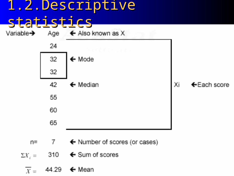
1.1.2.Descriptive statistics2.Descriptive statistics

1.1.3.Descriptive statistics3.Descriptive statistics MeanMean - the arithmetic average of the scores in a

sample distribution. MedianMedian - the point on a scale of measurement below

which fifty percent of the scores fall. ModeMode - the most frequently occurring score in a

distribution. RangeRange - The difference between the highest and

lowest score (high-low). VarianceVariance - The average of the squared deviations

between the individual scores and the mean. The larger the variance the more variability there is among the scores.

Standard deviationStandard deviation - The square root of variance. It provides a representation of the variation among scores that is directly comparable to the raw scores.

1.1.4.Descriptive statistics4.Descriptive statistics

22..SStatistical Hypothesis Testing tatistical Hypothesis Testing Hypothesis testingHypothesis testing is used to establish whether

the differences exhibited by random samples can be inferred to the populations from which the samples originated.

Chain of reasoning for inferential statistics Chain of reasoning for inferential statistics Sample(s) must be randomly selected Sample(s) must be randomly selected Sample estimate is compared to Sample estimate is compared to

underlying distribution of the same size underlying distribution of the same size sampling distribution sampling distribution

Determine the probability that a sample Determine the probability that a sample estimate reflects the population parameterestimate reflects the population parameter

22..1.S1.Statistical Hypothesis Testing tatistical Hypothesis Testing The Normal Distribution.The Normal Distribution. Although there are

numerous sampling distributions used in hypothesis testing, the normal distribution is the most common example of how data would appear if we created a frequency histogram where the x axis represents the values of scores in a distribution and the y axis represents the frequency of scores for each value.

Most scores will be similar and therefore will group near the center of the distribution.

Some scores will have unusual values and will be located far from the center or apex of the distribution. .

22..1.The Normal Distribution1.The Normal DistributionProperties of a normal distribution: Forms a symmetric bell-shaped curve 50% of the scores lie above and 50% below the midpoint

of the distribution Curve is asymptotic to the x axis Mean, median, and mode are located at the midpoint of

the x axis

2.2.Overview of the hypothesis testing 2.2.Overview of the hypothesis testing processprocess State the null hypothesis

Look at the data and decide on an appropriate statistical test.

Compute the statistical test, look at P value.

P value < , reject null hypothesis. Report P value, estimated effect, and precision of estimate.

P value > , fail to reject null hypothesis. Report P value, power of study, and how big an effect you might have missed.

2.2.Overview of the hypothesis 2.2.Overview of the hypothesis testing processtesting processState the HypothesisState the Hypothesis Null Hypothesis (Ho):Null Hypothesis (Ho): There is no difference between

___ and ___. Alternative Hypothesis (Ha):Alternative Hypothesis (Ha): There is a difference

between __ and __. Rejection CriteriaRejection Criteria This determines how different the parameters and/or

statistics must be before the null hypothesis can be rejected. This "region of rejection" is based on alphaalpha () - the error associated with the confidence level. The point of rejection is known as the critical valuecritical value.

For the medical For the medical investigationsinvestigations use value use value = 0,05 = 0,05 (5%)(5%).

2.2.Overview of the hypothesis 2.2.Overview of the hypothesis testing processtesting process

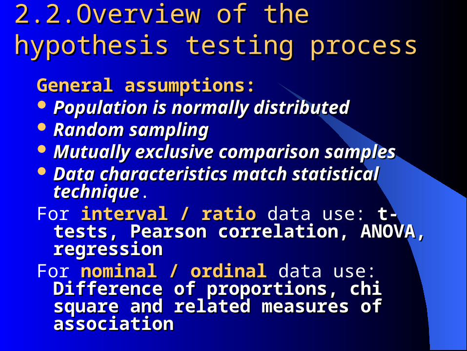
General assumptions:General assumptions: Population is normally distributed Population is normally distributed Random sampling Random sampling Mutually exclusive comparison samples Mutually exclusive comparison samples Data characteristics match statistical Data characteristics match statistical

techniquetechnique.For intervalinterval / / ratioratio data use: t-tests, Pearson t-tests, Pearson

correlation, ANOVA, regressioncorrelation, ANOVA, regression For nominalnominal / / ordinalordinal data use: Difference of Difference of

proportions, chi square and related proportions, chi square and related measures of associationmeasures of association

2.2.Overview of the hypothesis testing process2.2.Overview of the hypothesis testing processAre data categorical or continuous?

Categorical data: compare proportions in groups.

Continuous data: compare means or medians in groups

Two or more groups, compare by chi-square test.

How many groups?

Two groups; normal data, same spread?

Normal data; use t test.

Non-normal data; use Wilcoxon test.

Three+ groups; normal data?

Normal data; use ANOVA

Non-normal data; use Kruskal Wallis

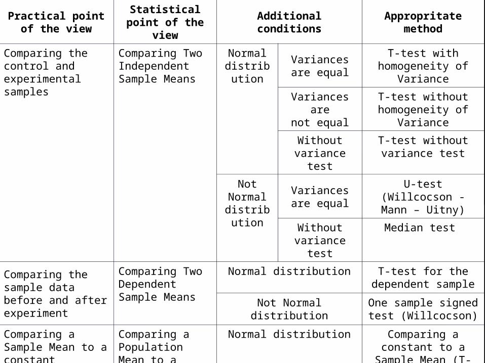
Practical point of the view

Statistical point of the view

Additional conditions Appropritate method

Comparing the control and experimental samples

Comparing Two Independent Sample Means

Normal distribution

Variances are equal

T-test with homogeneity of Variance

Variances arenot equal

T-test without homogeneity of Variance

Without variance test

T-test without variance test

Not Normal

distribution

Variances are equal

U-test (Willcocson - Mann – Uitny)

Without variance test

Median test

Comparing the sample data before and after experiment

Comparing Two Dependent Sample Means

Normal distribution T-test for the dependent sample

Not Normal distribution One sample signed test (Willcocson)

Comparing a Sample Mean to a constant

Comparing a Population Mean to a Sample Mean

Normal distributionComparing a constant to a Sample Mean (T-test)

Not Normal distribution Gupt signed test

Comparing the parameter diffusion in two samples

Comparing Two Independent Sample Variances

Normal distribution Computing F-ratio

Not Normal distribution Zigel-Tiuky, Mozes tests

2.3. One tail test with rejection 2.3. One tail test with rejection region on leftregion on leftThe rejection region will be in the left tail.

2.3. Two tail test with rejection 2.3. Two tail test with rejection region in both tailsregion in both tailsThe rejection region is split equally

between the two tails.

2.3. Summary of One- and 2.3. Summary of One- and Two-Tail Tests…Two-Tail Tests…

One-Tail Test

(left tail)

Two-Tail Test

One-Tail Test

(right tail)

Hypothesis testing offers us two choices:Hypothesis testing offers us two choices:

1. Conclude that the difference between the two groups is so large that it is unlikely to be due to chance alone. Reject the null hypothesis and conclude that the groups really do differ.

2. Conclude that the difference between the two groups could be explained just by chance. Accept the null hypothesis, at least for now.

Note that you could be making a mistake, either way!

You could reject the null hypothesis, publish a paper saying “men and women really differ” or “new treatment is really better than old”, and be wrong. This is called a Type I error. Type I error can only happen if you reject the null and conclude there is something happening. Hard to undo once published.

2.4.Conclusions of a Test of Hypothesis…2.4.Conclusions of a Test of Hypothesis…

You could also make a mistake if you fail to reject the null hypothesis when there really is a difference. This is called a Type II error. A Type II error could happen if

• The difference is so small that it doesn’t matter much or is very hard to detect.

• The difference is big enough to care about, but your sample size was just too small to tell you much. This is called an “uninformative null finding”.

Some people and some journals don’t like to publish null findings. It is important, however, to publish them if the results are informative (based on enough data to rule out large differences).

For example, some people have claimed women are at higher risk of Alzheimer’s disease. Careful analysis in large studies shows, however, that women have more AD only because they live longer. That is an important finding and needed to be published.

2.4.Conclusions of a Test of Hypothesis…2.4.Conclusions of a Test of Hypothesis…

22..5.Outcomes in hypothesis testing5.Outcomes in hypothesis testing The four possible outcomes in hypothesis

testing:

DECISION

Actual Population Comparison

Null Hyp. True(there is no difference)

Null Hyp. False(there is a difference)

Rejected Null Hypothesis

Type I error (alpha)

Correct Decision

Did not Reject Null

Correct Decision Type II Error

When conducting statistical tests with computer software, the exact probability of a Type I error is calculated. It is presented in several formats but is most commonly reported as "p <p <" or "SigSig." or "SignifSignif." or "SignificanceSignificance." The following table links p values with a benchmark alpha of 0.05:

p < Alpha Probability of Type I Error Final Decision

0.05 0.05 5% chance difference is not significant

Statistically signif.


Not statistically signif.


Statistically signif.


Not statistically signif.

22..5.Outcomes in hypothesis testing5.Outcomes in hypothesis testing

2.5.Interpreting the p-value…2.5.Interpreting the p-value…Overwhelming Evidence(Highly Significant)

Strong Evidence(Significant)

Weak Evidence(Not Significant)

No Evidence(Not Significant)

0 .01 .05 .10

p=.0069

2.5.Conclusions of a Test of 2.5.Conclusions of a Test of Hypothesis…Hypothesis… If we reject the null hypothesis, we conclude that there

is enough evidence to infer that the alternative hypothesis is true.

If we fail to reject the null hypothesis, we conclude that there is not enough statistical evidence to infer that the alternative hypothesis is true. This does not mean that we have proven that the null hypothesis is true!

Keep in mind that committing a Type I error OR a Type II error can be VERY bad depending on the problem.

33. . The STATISTICA usage The STATISTICA usage exampleexample

• Correlation

• Hypothesis Testing

33. . The STATISTICA usage exampleThe STATISTICA usage exampleThis example is based on the Adstudy.sta example data file that is included with

STATISTICA.

This data file contains 25 variables and 50 cases. These data were collected in an advertising study where male and female respondents evaluated two advertisements. Respondents' gender was coded in variable 1 (Gender: 1=male, 2=female).

Each respondent was randomly assigned to view one of the two ads (Advert: 1=Coke®, 2=Pepsi®). They were then asked to rate the appeal of the respective ad on 23 different scales (Measure01 to Measure23). On each of these scales, the respondents could give answers between 0 and 9.

33. . The STATISTICA usage exampleThe STATISTICA usage example Start STATISTICA and open the data file Adstudy.sta via the File - Open menu; it is

installed in the /Examples/Datasets directory of STATISTICA. You can also open data files from most Startup Panels of each statistical module. For example, select Basic Statistics/Tables from the Statistics menu to display the Basic Statistics and Tables Startup Panel.

Click the Open Data button to display the Select Spreadsheet dialog; in that dialog click the Files button to select the datafile

33. . The STATISTICA - The STATISTICA - CorrelationsCorrelations First, check whether ratings on individual scales are correlated (in other words, whether

some scales measured the "same thing"). In the Basic Statistics and Tables Startup Panel, select Correlation matrices and then click the OK button (or you can double-click on Correlation matrices).

The Product-Moment and Partial Correlations dialog will be displayed. You can select variables either in one list (i.e., a square matrix) or in two lists (rectangular

matrix). For this example, click the One variable list button and the standard variable selection dialog will be displayed. Select all variables (e.g., click the Select all button in the variable selection dialog), and then click the Summary button to display a spreadsheet with the correlations.

33. . The STATISTICA - The STATISTICA - CorrelationsCorrelations Highlighting significant correlations. By default, the spreadsheet will show all correlation

coefficients that are significant at p<.05 (two-tailed) in a different (highlight) color. You can specify the significance (alpha) level used to highlight significant correlation coefficients in the spreadsheet. To change the alpha level, display the Product-Moment and Partial Correlations dialog again, click the Options tab, and change the p-level for highlighting value to, for example, .001. Click the Summary button again to display the updated results spreadsheet in which all correlations that meet this significance criterion will be highlighted. This high correlation indicates that those two rating scales may measure similar aspects of the viewers' perception of the advertisement (although one is a decreasing and the other an increasing measure of that aspect).

33. . The STATISTICA - The STATISTICA - CorrelationsCorrelations The Display detailed table of results option button on the Options tab of the

Product-Moment and Partial Correlations dialog is only available if 20 or fewer variables have been selected for the analysis, since a large amount of information is automatically produced for each correlation. When you select this option, a spreadsheet will be displayed, containing relevant descriptive statistics, the correlation coefficient, p-value and pairwise N, as well as the slopes and intercepts of the regression equations for each variable in the correlation.

This option should be used to examine only specific correlations (and not for exploratory data analysis), because 22 spreadsheet cells are occupied for each correlation coefficient in this format; thus, a 20x20 correlation matrix will produce a spreadsheet with 8,800 cells. As you can see above, the correlation for Measure05 and Measure09 is highly significant (p=.0006), which means that the error associated with accepting this result is only 6 in 10,000.

33. . The STATISTICA - The STATISTICA - HTHT Differences between Means (t-Test). In the next step of the analysis, the possibility

of differences in response patterns between males and females will be examined. Specifically, males may use some rating scales in a different way, resulting in higher or lower ratings on some scales. The t-test for independent samples will be used to identify such potential differences. The sample of males and females will be compared regarding their average ratings on each scale. Return to the Basic Statistics and Tables Startup Panel and select t-test, independent, by groups in order to display the T-Test for Independent Samples by Groups dialog.

Next, click the Variables button to display the standard variable selection dialog. Here, you can select both the independent (grouping) and dependent variables for the analysis. For this example, select (highlight) variables 3 through 25 (the variables containing the responses) as the dependent variables; select variable Gender as the independent variable.

33. . The STATISTICA - The STATISTICA - HTHT Once you have made the grouping variable selection, STATISTICA will automatically

propose the codes used in that variable to identify the groups to be compared (in this cases the codes are Male and Female). You can double-click on either the Code for Group 1 or Code for Group 2 boxes to display the Variable Codes dialog in which you can review and select the codes for each group.

Many other procedures are available on the Advanced tab on the T-Test for Independent Samples by Groups dialog. Before performing the analysis, you can graphically view the distribution of the variables via the graphics options on this dialog. For example, click the Box & whisker plot button (and select the Mean/SE/1.96*SE option button in the Box-Whisker Type dialog) to produce box and whisker plots categorized by the grouping variable, one plot for each of the dependent variables. Similarly, click the Categorized Histograms button to produce categorized (by the grouping variable) histograms. If your current output (see Output Manager) is directed to workbooks (default), all graphs can quickly be reviewed.

33. . The STATISTICA - The STATISTICA - HTHT Once you have made the grouping variable selection, STATISTICA will automatically propose the codes

used in that variable to identify the groups to be compared (in this cases the codes are Male and Female). You can double-click on either the Code for Group 1 or Code for Group 2 boxes to display the Variable Codes dialog in which you can review and select the codes for each group.

Many other procedures are available on the Advanced tab on the T-Test for Independent Samples by Groups dialog. Before performing the analysis, you can graphically view the distribution of the variables via the graphics options on this dialog. For example, click the Box & whisker plot button (and select the Mean/SE/1.96*SE option button in the Box-Whisker Type dialog) to produce box and whisker plots categorized by the grouping variable, one plot for each of the dependent variables. Similarly, click the Categorized Histograms button to produce categorized (by the grouping variable) histograms. If your current output (see Output Manager) is directed to workbooks (default), all graphs can quickly be reviewed.

Now, click the Summary button to display the spreadsheet of t-test results.

33. . The STATISTICA - The STATISTICA - HTHT Reviewing the t-test output. The quickest way to explore the table is to examine the fifth

column (p-levels) and look for p-values that are less than the conventional significance level of .05 (see Elementary Concepts). For the vast majority of dependent variables, the means in the two groups (Males and Females) are very similar. The only variable for which the t-test meets the conventional significance level of .05 is Measure07 for which the p-level is equal to .0087. A look at the columns containing the means (see the first two columns) reveals that males used much higher ratings on that scale (5.46) than females (3.63). The possibility that this difference was obtained by chance cannot be entirely excluded, although assuming that the test is valid (see below), it appears unlikely, because a difference at that significance level is expected to occur by chance (approximately) 9 times per 1,000 (thus, less than only 1 time per 100). This result will be examined further, but first, look at the box and whisker plot for this variable.

33. . The STATISTICA - The STATISTICA - HTHT Go back to the box-whisker plot that you previously produced. Then select the graph for variable

Measure07; double-click on the graph to display the All Options dialog, select the Plot: Box/Whisker tab, and set the Whisker value drop-down box to Std Dev (standard deviations).

The graph shows something unexpected: The variation in the group of females appears much larger than in males. If the variation of scores within the two groups is in fact reliably different, then one of the theoretical assumptions of the t-test is not met (see the Introductory Overview), and you should treat the difference between the means with particular caution. Also, differences in variation are typically correlated with the means, that is, variation is usually higher in groups with higher means. However, something opposite appears to be happening in the current case. In situations like this one, experienced researchers would suspect that the distribution of Measure07 might not be normal (in males, females, or both). However, first look at the test of variances to see whether the difference visible on the graph is reliable.

44. . Regression Analysis BasicsRegression Analysis Basics

Understanding Curve Fitting.MS Excel trendline feature.

3.1. Understanding 3.1. Understanding Curve FittingCurve FittingCurve fittingCurve fitting is the process of trying to find

the curve (which is represented by some model equation) that best represents the sample data, or more specifically the relationship between the independent and dependent variables in the dataset.

When the results of the curve fit are to be used for making new predictions of the dependent variable, this process is known as regressionregression analysis analysis.

3.1. Understanding 3.1. Understanding Curve FittingCurve Fitting The Linear Linear trendline uses the equation:

у = k • x + b,у = k • x + b,

– where kk and bb are parameters to be determined during the curve-fitting process.

The LogarithmicLogarithmic trendline uses the equation:

у = у = сс • ln(x) + b, • ln(x) + b,

– where cc and bb are parameters to be determined during the curve-fitting process.

3.1. Understanding 3.1. Understanding Curve FittingCurve Fitting The Power Power trendline uses the equation:

у = с • ху = с • хbb,,


The ExponentialExponential trendline uses the equation:

у = с • еу = с • еbb • х, • х,


3.1. Understanding 3.1. Understanding Curve FittingCurve Fitting

The Polynomial Polynomial trendlines use the equation:

у = у = bb + + сс11 х + х + сс22 х х22 + + сс33 х х33 + + сс44 х х44 + + сс55 х х55 +с +с66 х х66

– where the cc-coefficients and bb are

parameters of the curve fit. Excel supports

polynomial fits up to sixth orderup to sixth order.

3.2. 3.2. Multiple Regression ExampleMultiple Regression Example Data File. This example is based on the data file Poverty.sta. Open this data

file via the File - Open menu; it is in the /Examples/Datasets directory of STATISTICA. The data are based on a comparison of 1960 and 1970 Census figures for a random selection of 30 counties. The names of the counties were entered as case names.

Research Question. Now, analyze the correlates of poverty, that is, the variables that best predict the percent of families below the poverty line in a county. Thus, you will treat variable 3 (Pt_Poor) as the dependent or criterion variable, and all other variables as the independent or predictor variables.

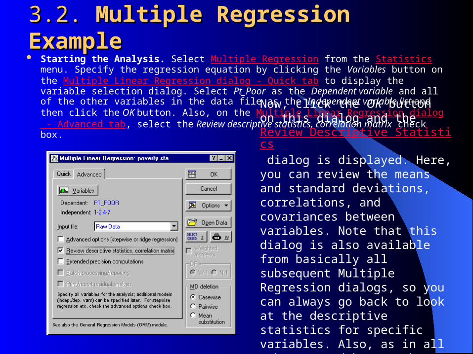
3.2. 3.2. Multiple Regression ExampleMultiple Regression Example Starting the Analysis. Select Multiple Regression from the Statistics menu. Specify

the regression equation by clicking the Variables button on the Multiple Linear Regression dialog - Quick tab to display the variable selection dialog. Select Pt_Poor as the Dependent variable and all of the other variables in the data file as the Independent variable list and then click the OK button. Also, on the Multiple Linear Regression dialog - Advanced tab, select the Review descriptive statistics, correlation matrix check box.

Now, click the OK button on this dialog and the Review Descriptive Statistics dialog is displayed. Here, you can review the means and standard deviations, correlations, and covariances between variables. Note that this dialog is also available from basically all subsequent Multiple Regression dialogs, so you can always go back to look at the descriptive statistics for specific variables. Also, as in all other spreadsheets, there are numerous graphs available.

3.2. 3.2. Multiple Regression ExampleMultiple Regression Example Specifying the Multiple Regression. Now click the OK button on the Review

Descriptive Statistics dialog to perform the regression analysis and display the Multiple Regression Results dialog. A standard regression (which includes the intercept) will be performed.

Reviewing Results. The text area of the Multiple Regression Results dialog is displayed below. Overall, the multiple regression equation is highly significant (refer to Elementary Concepts for a discussion of statistical significance testing). Thus, given the independent variables, you can "predict" poverty better than what would be expected by pure chance alone.

Regression coefficients. In order to learn which of the independent variables contribute most to the prediction of poverty, examine the regression (or B) coefficients. Click the Summary: Regression results button on the Quick tab to display a spreadsheet with those coefficients.

3.2. 3.2. Multiple Regression ExampleMultiple Regression Example This spreadsheet shows the standardized regression coefficients (Beta) and the raw

regression coefficients (B). The magnitude of these Beta coefficients allow you to compare the relative contribution of each independent variable in the prediction of the dependent variable. As is evident in the spreadsheet shown above, variables Pop_Chng, Pt_Rural, and N_Empld are the most important predictors of poverty; of those, only the first two variables are statistically significant. The regression coefficient for Pop_Chng is negative; the less the population increased, the greater the number of families who lived below the poverty level in the respective county. The regression weight for Pt_Rural is positive; the greater the percent of rural population, the greater the poverty level.

ConclusionConclusion

In this lecture was described next questions:Descriptive statistics.Statistical hypothesis testing.Regression analysisThe STATISTICA usage example.

LiteratureLiterature

Electronic documentation on to the TDMU server:http://www.tdmu.edu.te.uahttp://www.tdmu.edu.te.ua

lections №5 using statistica fot the statistical hypothesis testing

Documents

values of scores

sample distribution

frequency of scores

standardized scores

individual scores

scores fall

raw scores

levels of data