lect 08 probability theory - brown university

CSCI 2570 Introduction to

Nanocomputing

Probability Theory

John E Savage

Lect 08 Probability Theory CSCI 2570 @John E Savage 2

The Role of Probability The manufacture of devices with nanometer-scale dimensions will necessarily introduce randomness into these devices.

Some device dimensions are so small that their position cannot be accurately controlled

For this reason, probability theory will play a central role in this area


Sample SpacesProbabilities estimate the frequency of outcomes of random experiments.

Outcomes can be from a finite or countable sample space (set) Ω of events or be tuplesdrawn over reals R.

Coin toss: Ω = H,TPackets to a URL per day: Ω = N (positive integers)Rain in cms/month in Prov.: Ω = R (reals)Rain and sunshine/month: Ω = R2


Probability SpaceSample space: all possible outcomes

Events: A family F of subsets of sample space Ω.E.g. Ω = H,T3, F0 = TTT, HHT, HTH, THH (Even no. Hs). F1 = HTT, THT, TTH, HHH (Odd no. Hs).

Events are mutually exclusive if they are disjoint. E.g. F0 and F1 above.

A probability distribution is a function

The probability distribution assigns a probability0 ≤ P(E) ≤ 1 to each event E.


Properties of Probability Function

For any event E in Ω, 0 ≤ P(E) ≤ 1.

P(Ω) = 1

For any finite or countably infinite sequence of disjoint events E1, E2, …


Probability Distributions

If Ω = Rn, probability density p(x1,…xn) can be integrated over a volume to give a probability. E.g.


Sets of Events

Joint probability P(A B) = Notation: P(A,B) = P(A B)

Probability of a union P(A B) =P(A B) = P(A) + P(B) – P(A B)

Complement of event A: A = Ω–A.P(A A)=1


Probabilities of Events

If events A and B are mutually exclusiveP(A B) = 0P(A B) = P(A) + P(B)

Conditional probability of A given B, P(A/B) = P(A,B)/P(B) or P(A,B) = P(A/B)P(B).

Events A and B are statistically independentif P(A/B) = P(A), i.e., P(A,B) = P(A)P(B)


Marginal Probability

Given a sample space Ω = K2 containing pairs of events Ai,Bj over K, the marginalprobability is P(A) = ∑j P(A,Bj), where Bj are mutually exclusive.


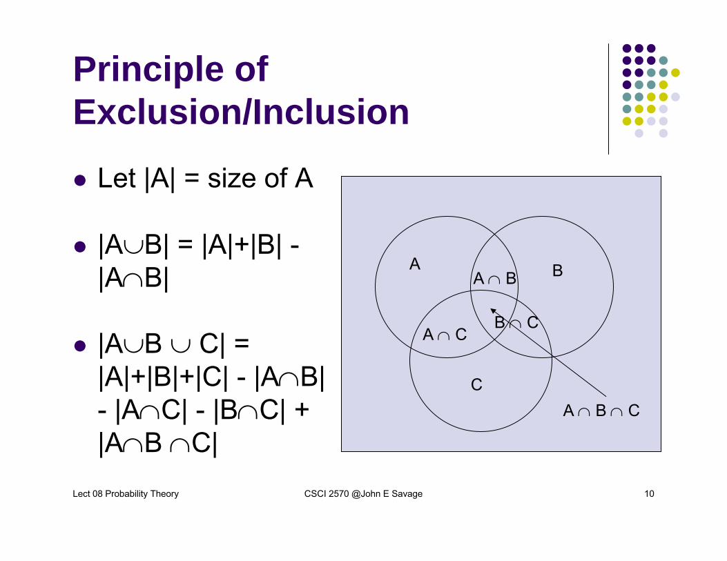
Principle of Exclusion/Inclusion

Let |A| = size of A

|A∪B| = |A|+|B| -|A∩B|

|A∪B ∪ C| = |A|+|B|+|C| - |A∩B| - |A∩C| - |B∩C| + |A∩B ∩C|

A B

C

B ∩ CA ∩ C

A ∩ B

A ∩ B ∩ C


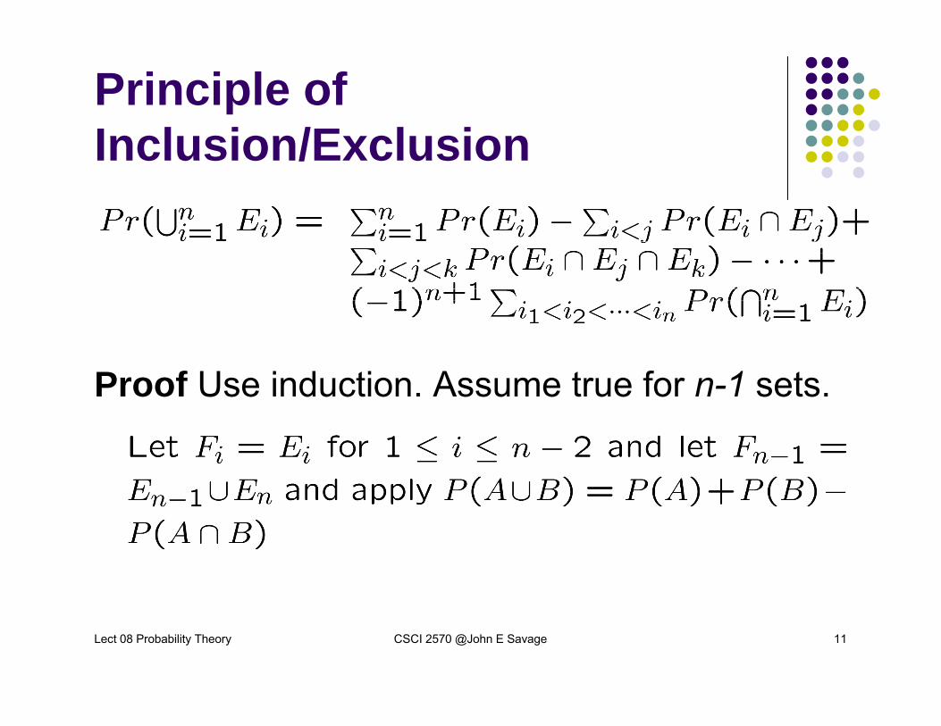
Principle of Inclusion/Exclusion

Proof Use induction. Assume true for n-1 sets.


Application of Inclusion/Exclusion

For odd, (-1)l+1 = 1

For even , (-1)l+1 = -1


Special Application of Inclusion/Exclusion


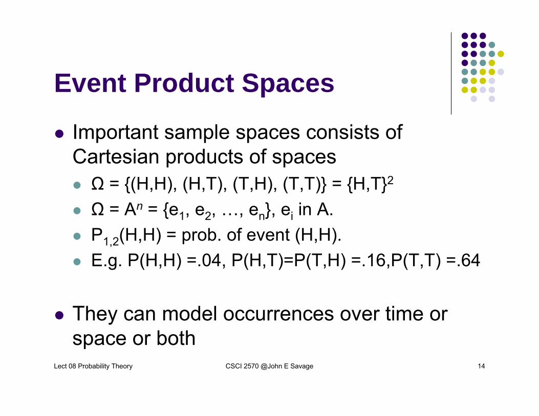
Event Product Spaces

Important sample spaces consists of Cartesian products of spacesΩ = (H,H), (H,T), (T,H), (T,T) = H,T2

Ω = An = e1, e2, …, en, ei in A.P1,2(H,H) = prob. of event (H,H).E.g. P(H,H) =.04, P(H,T)=P(T,H) =.16,P(T,T) =.64

They can model occurrences over time or space or both


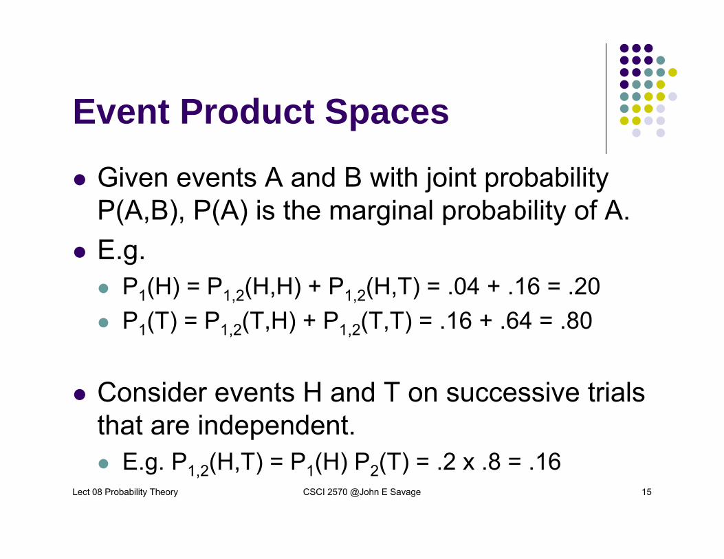
Event Product Spaces

Given events A and B with joint probability P(A,B), P(A) is the marginal probability of A.E.g.

P1(H) = P1,2(H,H) + P1,2(H,T) = .04 + .16 = .20P1(T) = P1,2(T,H) + P1,2(T,T) = .16 + .64 = .80

Consider events H and T on successive trials that are independent.

E.g. P1,2(H,T) = P1(H) P2(T) = .2 x .8 = .16


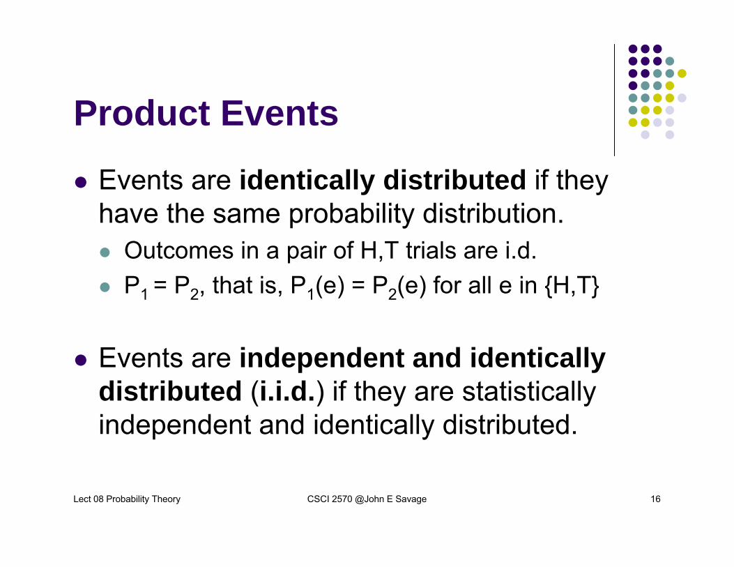
Product Events

Events are identically distributed if they have the same probability distribution.

Outcomes in a pair of H,T trials are i.d.P1 = P2, that is, P1(e) = P2(e) for all e in H,T

Events are independent and identically distributed (i.i.d.) if they are statistically independent and identically distributed.


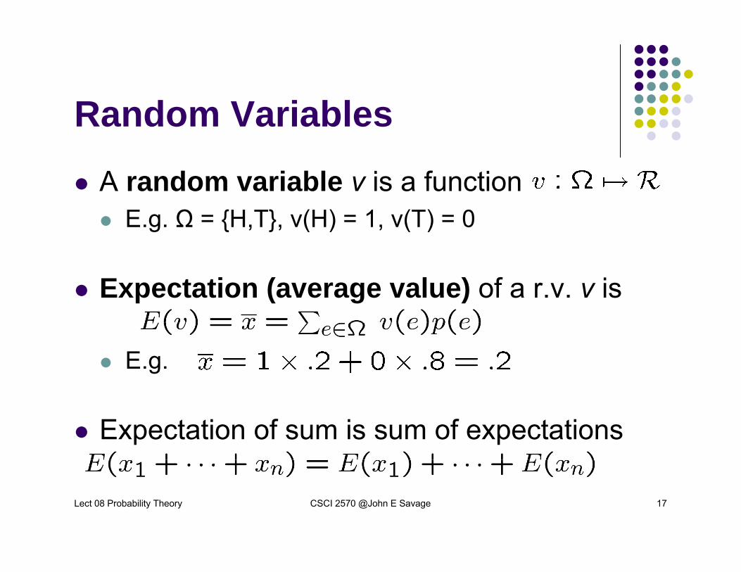
Random Variables

A random variable v is a functionE.g. Ω = H,T, v(H) = 1, v(T) = 0

Expectation (average value) of a r.v. v is

E.g.

Expectation of sum is sum of expectations


Geometric Random Variable


Moments of Random Variables

Second moment of a r.v.

kth moment or a r.v.

Variance

Standard deviation


Examples of Probability Distributions

Uniform: P(k) = 1/n for 1 ≤ k ≤ n

Binomial: n i.i.d. trials, Ω =H,Tn, P(H) = αand P(T) = β = 1- α. P(k) = Pr(k H’s occur)

Poisson:Is limit of binomial when and n large.


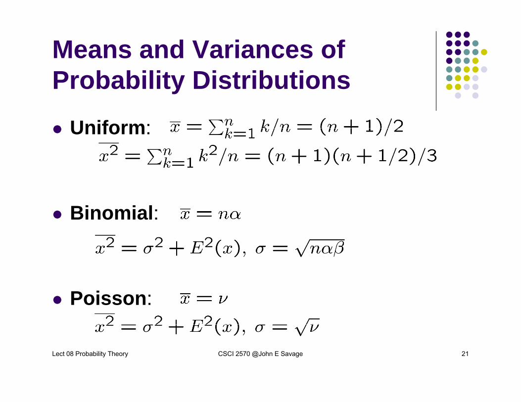
Means and Variances of Probability Distributions

Uniform:

Binomial:

Poisson:


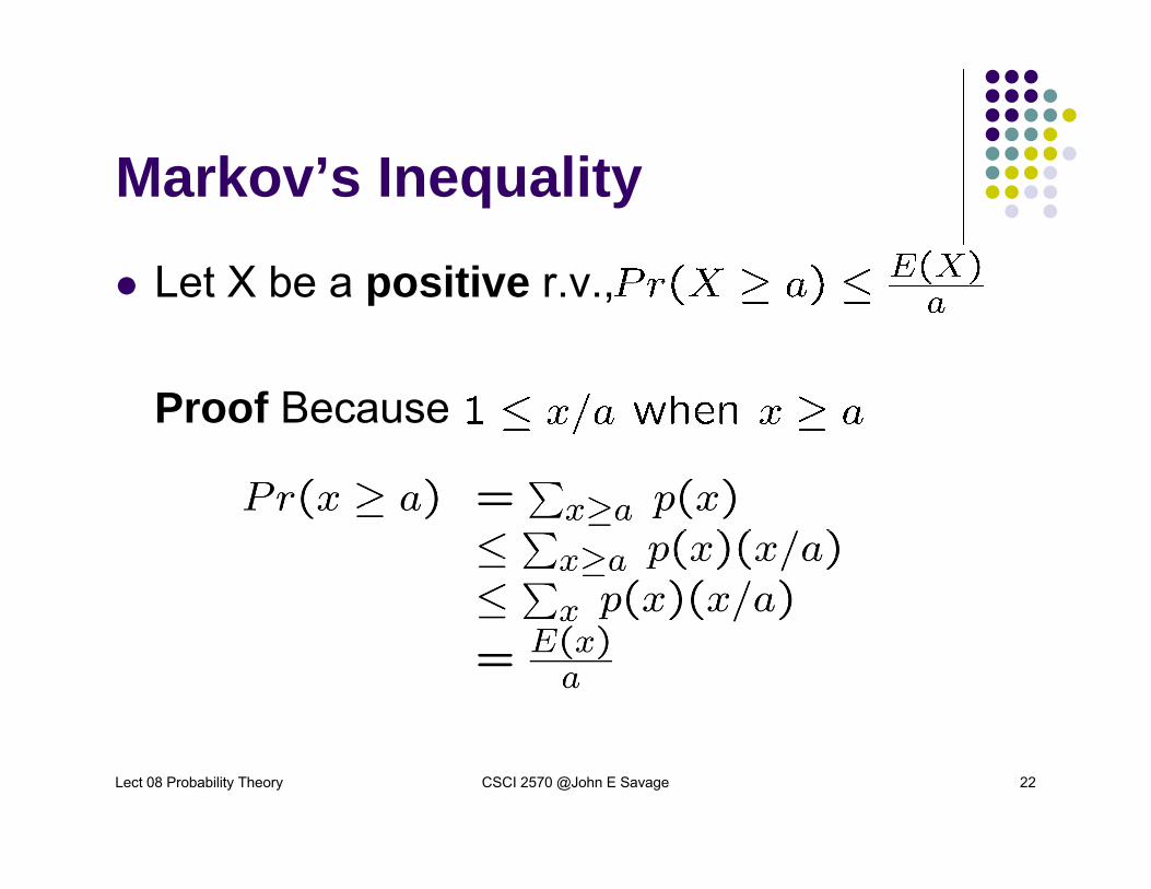
Markov’s Inequality

Let X be a positive r.v.,

Proof Because


Chebyshev’s Inequality

Let X be a r.v.

Proof Note


Moment Generating Function

is a function that can be used to compute moments and Chernoff bounds on tails of probabilities, i.e.


Moment Generating Functions

Uniform:

Binomial:

Poisson:


Chernoff Bound

Let X be a r.v.

Proof Because


Bounding Tails of a Binomial

Markov

Chebyshev

Chernoff


Chernoff Bound on Binomial Distribution

Choose t = t0 to minimize boundNote that is convex because its second derivative is positive.Thus, at t0 the first derivative is zero.That is and

Here

t0


Comparison of Bounds

n=100, α=.5, β=.5, a=70, E(x)=50, Var(x) = 5Markov:Chebyshev:implies Chernoff:

impliesExact:


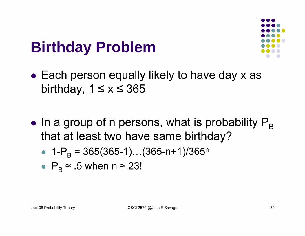
Birthday Problem

Each person equally likely to have day x as birthday, 1 ≤ x ≤ 365

In a group of n persons, what is probability PBthat at least two have same birthday?

1-PB = 365(365-1)…(365-n+1)/365n

PB ≈ .5 when n ≈ 23!


Balls in Bins

m balls thrown into n bins independently and uniformly at randomHow large should m be to ensure that all bins contain at least one ball with prob. ≥ 1-ε?Coupon collector problem:

C coupon typesEach box equally likely to contain any coupon typeHow many boxes should be purchased to collect all coupons with probability at least 1-ε?


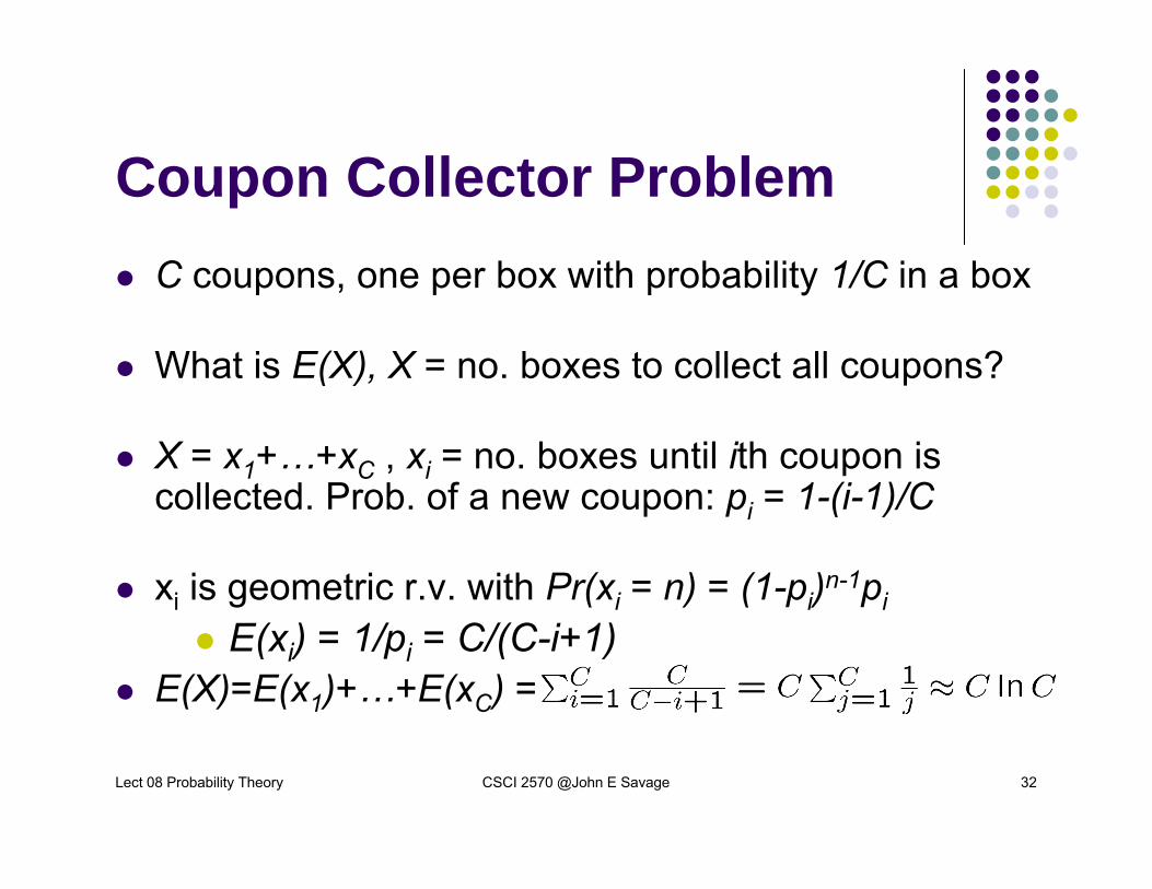
Coupon Collector ProblemC coupons, one per box with probability 1/C in a box

What is E(X), X = no. boxes to collect all coupons?

X = x1+…+xC , xi = no. boxes until ith coupon is collected. Prob. of a new coupon: pi = 1-(i-1)/C

xi is geometric r.v. with Pr(xi = n) = (1-pi)n-1pi

E(xi) = 1/pi = C/(C-i+1)E(X)=E(x1)+…+E(xC) =


Coupon Collector Problem with Failures

In this model the probability that a coupon is not collected is 1-ps. The probability that a specific coupon is collected is ps/C.

Theorem Let T = no. trials to ensure all C coupons collected with probability = 1-ε in coupon collector problem with failures satisfies


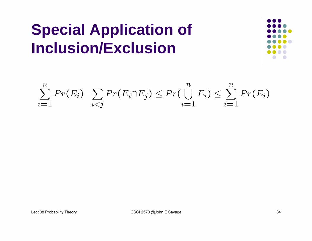
Special Application of Inclusion/Exclusion


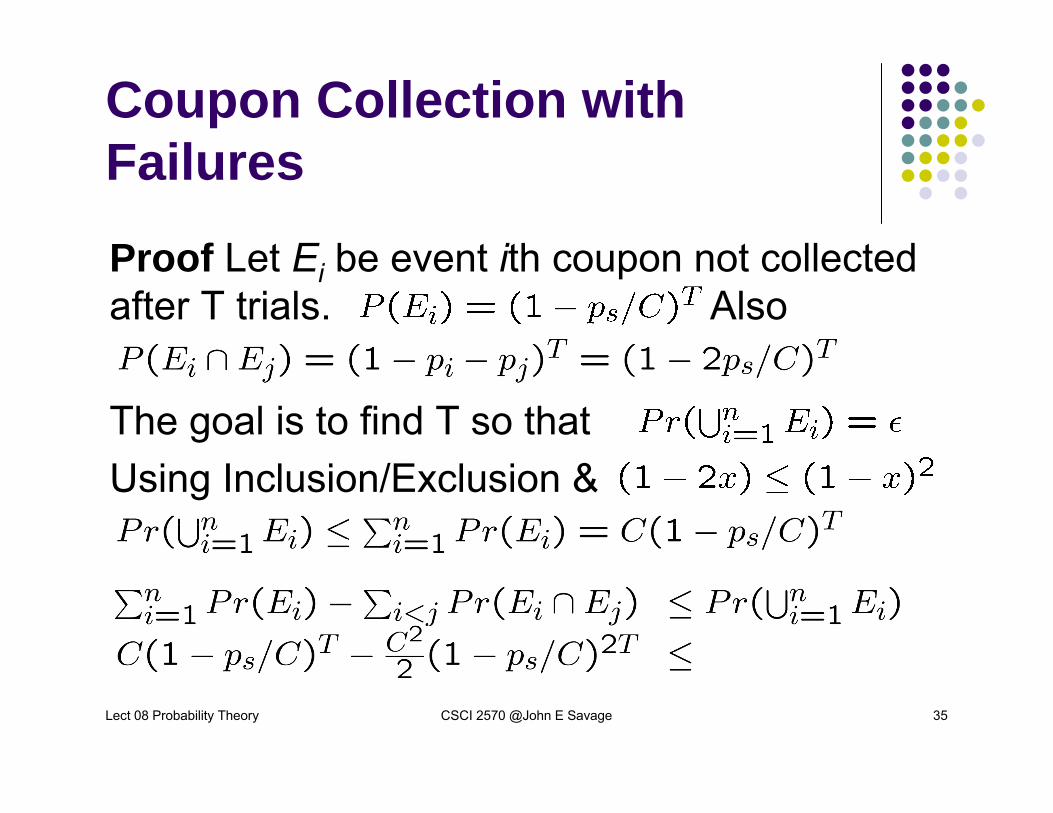
Coupon Collection with Failures

Proof Let Ei be event ith coupon not collected after T trials. Also

The goal is to find T so that Using Inclusion/Exclusion &


Coupon Collection with Failures

Then

Equivalently but this implies

Using

gives the desired result.


Conclusion

Methods of bounding tails of probability distributions can be very useful.

lect 08 probability theory - brown university

Documents