lec16 modules
TRANSCRIPT

Watershed Management Prof. T. I. Eldho
Department of Civil Engineering Indian Institute of Technology, Bombay
Module No. # 04 Lecture No. # 16
Hydrologic Modeling
Namaste and welcome back to the video course on watershed management in module
number 4 - watershed modeling. Today, lecture number 16, we will discuss hydrologic
modeling. So, some of the important topics covered in today’s lecture include rainfall
runoff modeling, runoff process, physical modeling, distributed model.
(Refer Slide Time: 00:30)
Then some of the important key words for today’s lecture include rainfall runoff
modeling, physical modeling and distributed modeling.

(Refer Slide Time: 00:44)
So, as we discussed earlier, when we deal with the water as resources for a watershed,
we have to see the various processes what is happening for the transformation from
rainfall to runoff, for the precipitation to runoff.
So, we have already seen that various hydrological processes will be there between this
transformation from precipitation to runoff. Some of the important hydraulic processes
which we have already seen earlier is the interception by the vegetation, and then
evapotranspiration, then surface storage or depression storage, then the infiltration, then
interflow percolation, and then, surface runoff, and finally, coming back to the direct run
off. Then all these direct runoff from the overland flow runoff, it will be joined to the
channel for example, this is the watershed then you can see that from various small
channels finally, a big stream for the watershed and the runoff will be taking place
through the channel to the outlet of the watershed (Refer Slide Time: 01 14).
So, here also we may have to include the ground water storage, ground water processes.
So, mainly the surface water processes and the ground water process and surface water
processes, we can classify into the overland flow component and the channel flow
component.

Then, when we are looking for the hydrologic modeling we have to assess for the given
rainfall condition how much will be the runoff at any location of the watershed; either
the distributed way or as a lumped way at the outlet of the watershed.
Generally, at the outlet of the watershed we will be describing as in terms of a
hydrograph, where the hydrograph is the discharge versus time. So, you can see that if
this one is the given rainfall millimeter per hour, and then, correspondingly we can
identify how much will be the runoff as the hydrograph discharge versus time, at the
outlet of the watershed or in the case of distributed model at any location of the
watershed.
(Refer Slide Time: 03:01)
So, that way as we discussed earlier we have various components as far as within the
transformation from the rainfall to runoff. We have already seen how to construct a
watershed model in the previous lectures. First we have to develop a conceptual model
for the watershed including watershed delineation and the consideration of various
parameters. Then we have to formulate the model so it can be either lumped model or the
black box model or the distributed model, so that aspect also we have seen in the last
lecture. Then once the model is formulated we have to develop the corresponding model
as a computer model or otherwise an analytical model.

Then, for the given problem, for the given area, we have to calibrate various parameters.
As far as the watershed is concerned and then for the given conditions for the given
intensity of rainfall or for given the event based rainfall conditions, either for event based
simulation or continuous simulation, we can do as far as the rainfall to runoff modeling
as a watershed model is concerned.
So, in all these aspects as we have already discussed there is an input function. So, input
function is mainly the rainfall as far as the watershed is concerned and then output
function is the runoff. So, runoff taking place at the outlet or at any location of a
watershed and the transformation function is the third one and that is mainly the various
hydrological processes taking place between the rainfall to runoff. As we already
discussed, so as far as surface runoff is concerned, when the rainfall is taking place we
can classify as far as runoff rainfall runoff is concerned, we can classify as the surface
runoff into overland flow and the channel flow.
After the losses or the or the transformations taking place, then we can see that the
overland flow, the on the overland flow the runoff starts and then through small channel
it will be coming to the main channel and then, the channel flow is taking place. So,
when we say that when we are going to model in watershed as far as rainfall runoff is
concerned, we have to consider various processes as so-called transformation taking
place and then we have to also consider the down water flow components if it is there.
Then, as far as surface flow is concerned, the model for the overland flow and the
channel flow.

(Refer Slide Time: 05:50)
So, both should be combined together to get the runoff at any location of the watershed
or the outlet of the watershed. Now, we will see more aspects as far as the hydrologic
modeling is concerned. We have seen the various classifications of the different types of
models and different kinds of concept-wise we have seen in the last lecture.
Now, in today’s lecture we will be discussing about the deterministic hydrologic
modeling. Here, depending upon the parameter considered for the watershed we can
classify into 3 main categories. So, first one is the lumped model, second one is a semi-
distributed model and the distributed model.

(Refer Slide Time: 06:57)
This classification is mainly based upon how we consider the various parameters; first
one is the lumped model. So, lumped model is concerned, when we are discussing a
particular watershed like this. This is our watershed which we are considering, so we can
see that here as far as the watershed is concerned we have to see the various parameters
are concerned here. Say, like the porosity or various other parameters like ne or the
saturated hydraulic conductivity like that various parameter will be lumping for the total
watershed as a single parameter. So, that process is called lumped model, so when we are
discussing for the given rainfall condition for the area is concerned there will be one
value for the total watershed.

(Refer Slide Time: 05:50)
That is so-called a lumped model. In the lumped model we consider the parameters
which are not varying, specially within the basin and response is evaluated only at the
outlet. So, the parameters the variation we are not considering but the parameters lumped
for the total watershed as a single parameter. Then this is without explicitly accounting
for the response of individual sub-basins. So, you can see that so here you can see that
there are various sub-basins; we can consider for this watershed this may be different
sub-basin for the considered watershed. Here, we are not considering the variations as far
as these sub-basins are concerned. But, here the parameters we lump for the total
watershed. So, here the parameters do not represent physical features of the hydrologic
processes.
Model parameters are the parameters which are area weighted; so it is an average, for the
various parameters for sub-basins are known. We consider the average of those
parameters and then we lump for the total watershed; so that way, when we are doing
these kinds of,… when you are using the lumped models. It is difficult to cope up with
the event based rainfall to runoff modeling but, we can do continuous simulation for a
daily basis or weekly basis or a monthly basis. What is happening, since most of the
parameters here are lumped?
Generally, when we use lumped models, the discharge prediction is only at the outlet and
so that way, we may not be able to identify what is really happening with respect to

spatially or with respect to time. What are the various hydrologic processes? How these
processes are varying we may not be able to identify when we use the lumped models.
But, of course, these lumped models have got a number of advantages. As I have listed
here, these models are very simple and then minimal data requirements and then easy to
use. Since the parameters are lumped, an average parameter we are taking; so that way
the modeling is very simple and data requirement is very less. In the model development
and running and getting results are much easier but of course, some of the disadvantages
like these lumped models we know, truly represents the various hydrological processes
taking place within the watershed.
So, that way we may not be able to capture what is happening with respect to the rainfall
to runoff various things happening. And, then how the runoff is distributed throughout
the watershed? All those things we may not be able to capture as far as the lumped
models are concerned. So, there are number of lumped models available.
(Refer Slide Time: 10:58)
We already discussed in the last lecture about the soil conservation curve number based
model. So, that is one of the commonly used lumped model for watershed modeling.
Then, other software like IHACRES; IHACRES then water balance models, etcetera. So,
these are some of the lumped models commonly used in practice. So, that is one category
of model; we have already seen the advantages and limitations of lumped models.
(Refer Slide Time: 11:30)
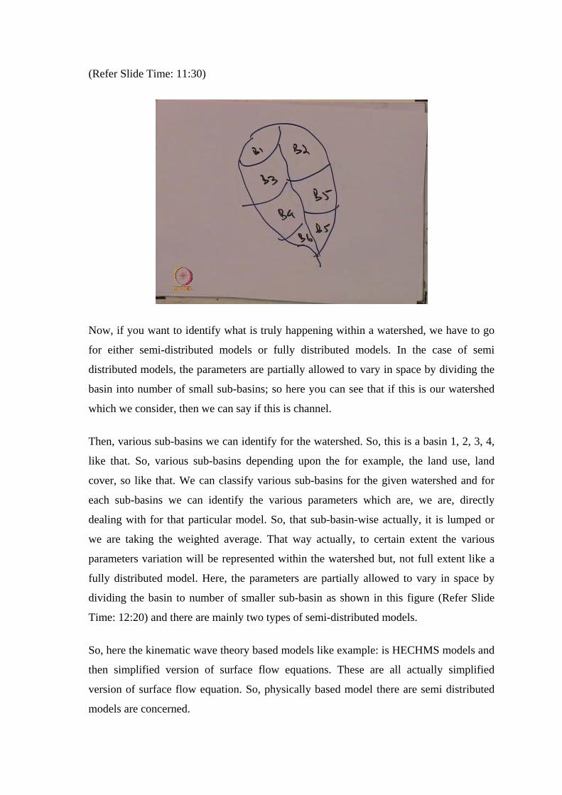
Now, if you want to identify what is truly happening within a watershed, we have to go
for either semi-distributed models or fully distributed models. In the case of semi
distributed models, the parameters are partially allowed to vary in space by dividing the
basin into number of small sub-basins; so here you can see that if this is our watershed
which we consider, then we can say if this is channel.
Then, various sub-basins we can identify for the watershed. So, this is a basin 1, 2, 3, 4,
like that. So, various sub-basins depending upon the for example, the land use, land
cover, so like that. We can classify various sub-basins for the given watershed and for
each sub-basins we can identify the various parameters which are, we are, directly
dealing with for that particular model. So, that sub-basin-wise actually, it is lumped or
we are taking the weighted average. That way actually, to certain extent the various
parameters variation will be represented within the watershed but, not full extent like a
fully distributed model. Here, the parameters are partially allowed to vary in space by
dividing the basin to number of smaller sub-basin as shown in this figure (Refer Slide
Time: 12:20) and there are mainly two types of semi-distributed models.
So, here the kinematic wave theory based models like example: is HECHMS models and
then simplified version of surface flow equations. These are all actually simplified
version of surface flow equation. So, physically based model there are semi distributed
models are concerned.
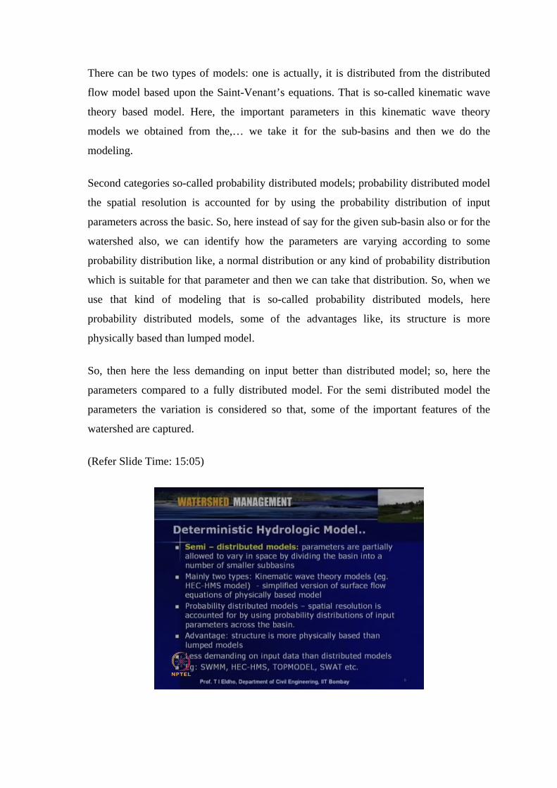
There can be two types of models: one is actually, it is distributed from the distributed
flow model based upon the Saint-Venant’s equations. That is so-called kinematic wave
theory based model. Here, the important parameters in this kinematic wave theory
models we obtained from the,… we take it for the sub-basins and then we do the
modeling.
Second categories so-called probability distributed models; probability distributed model
the spatial resolution is accounted for by using the probability distribution of input
parameters across the basic. So, here instead of say for the given sub-basin also or for the
watershed also, we can identify how the parameters are varying according to some
probability distribution like, a normal distribution or any kind of probability distribution
which is suitable for that parameter and then we can take that distribution. So, when we
use that kind of modeling that is so-called probability distributed models, here
probability distributed models, some of the advantages like, its structure is more
physically based than lumped model.
So, then here the less demanding on input better than distributed model; so, here the
parameters compared to a fully distributed model. For the semi distributed model the
parameters the variation is considered so that, some of the important features of the
watershed are captured.
(Refer Slide Time: 15:05)
So, here less demanding on input data than distributed models, some of the advantages
are like the features are somewhat represented and these parameters are not fully like
compared to fully distributed model. Here it is not the complete variation is taken care
but sub-basin ways variation is taken care. So, there are number of semi-distributed
model available literature like a SWMM model, storm water management model then,
HEC hydraulic engineering center hydraulic model, simulation HECHMS model. Then,
top model and then soil water assessment tool SWAT model. All these are somewhat
semi-distributed models. Here we can see that we consider for example SWAT model,
we consider the hydrologic response unit and for each response unit we take the
weighted average parameters.
(Refer Slide Time: 16:11)
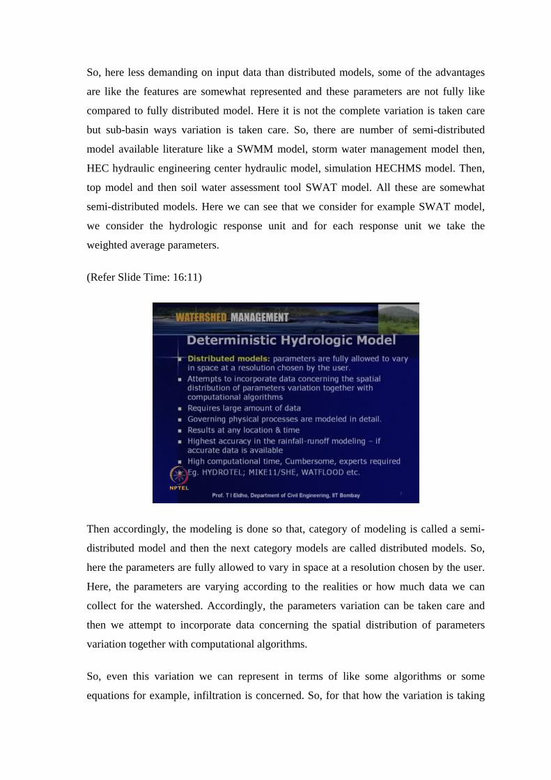
Then accordingly, the modeling is done so that, category of modeling is called a semi-
distributed model and then the next category models are called distributed models. So,
here the parameters are fully allowed to vary in space at a resolution chosen by the user.
Here, the parameters are varying according to the realities or how much data we can
collect for the watershed. Accordingly, the parameters variation can be taken care and
then we attempt to incorporate data concerning the spatial distribution of parameters
variation together with computational algorithms.
So, even this variation we can represent in terms of like some algorithms or some
equations for example, infiltration is concerned. So, for that how the variation is taking

place with respect to soil or with respect to the depth of soil. Like that we can have
various computational algorithms and so actually, these are truly the physical models
which is are representing the complete features of the watershed. But, some of the
disadvantage of these kinds of modeling include and requires large amount of data. We
need to capture the entire variations of the various parameters within the watershed either
through field investigations or through some that kind of equations. Then, some
advantages include the governing physical processes, are modeled in detail; so all the
aspects we can capture and then results at any location and at anytime when we are
dealing time depending modeling, the spatial variation we can obtain from rainfall
runoff. So, how much is the runoff at particular location or what is the depth of flow or
how the discharge variation is taking place? So, location and time base we can identify
and then if all the data are available in an accurate way, I mean, the data is accurate then
the results will be also accurate. So, highest accuracy in rainfall runoff modeling is
possible but, most of the time this is a big question mark; since, most of the time as far as
a watershed is concerned many of the parameters are varying drastically from one
location to another location.
Accordingly, it is very difficult to get all these parameter variations and then to get the
accurate data. As far as the parameters are concerned, it is not so easy; so that way the
accuracy of the model results will not be set to the expected levels. So, there will be lot
of variation. Since the data input is not accurate then obviously, results will not be also
accurate and then some other limitations like high computational time. When we are
going to run such models we need to run the computer for long time and then the
modeling will be cumbersome. Then that kind of models only experts can do; so that
means those who know how the modeling is done. And then, most of the time we have to
go for numerical modeling like a final difference or final terminal modeling; so the
experts only can easily do these kinds of modeling.

(Refer Slide Time: 16:11)
Some of the available software included like hydrotel modeling mike11 or mikeshe
models; then watflood model, etcetera. So, these are all physically based model where
we solved the Saint-Venant’s equations or the governing equations by considering the
conservation of mass or continuity equation and then momentum equations. Then, we
use a numerical tool like finite difference method or finite element methods and then we
develop this model by considering the various hydraulic processes like infiltration,
evapotranspiration, interception, interflow, groundwater flow component, etcetera.
(Refer Slide Time: 20:20)

Then we make this model; so as you can see so much of data is required to get accurate
results for these kinds of models. Now, we have come back to the physically based
watershed model, based upon the governing equations and within a based upon a system
approach. So, the main aim in physically based deterministic modeling is to gain better
understanding of hydrologic phenomena operating in a watershed and how changes in
watershed may affect these phenomena. So, this is what we are trying to do as far as
watershed modeling is concerned.
We want to understand the hydrologic phenomena operating and then if any changes are
proposed like, we constructing a check dam at particular location or we are going for
water harvesting measures. Then, what will happen? So, that way, that is our aim. As we
can see that all the variations or all the topography or the topological features or
geological features of the watershed is concerned, is so complex. Accordingly, this
modeling is also very complex. So, only thing is that we can using certain assumptions
we can, may go for a 1 dimensional, 2 dimensional modeling. Or, we can lump various
parameters or processes with respect to space and time and then we can simplify the
models.
Most of the physically based deterministic models generally, follow the loss of physics.
So, that means mainly in these kinds of models according to the poor mechanics theories
we use conservation of mass conservation of momentum and conservation of energy
principles. Out of this generally, we use conservation of mass and conservation of
momentum. So, conservation of mass, corresponding continuity equation and
conservation momentum, corresponding equation of motion and then equation of energy
or Bernoulli’s theorem we can utilize. One or more of these laws and several empirical
relations are used in physical model development. Generally, as far as the modeling is
concerned, we use these governing equations. But, to deal with various hydrological
processes between the transformation functions like a evaporation, evapotranspiration
then intersection, then infiltration, etcetera. So, various hydrologic processes are to be
considered.
So, that way we may have to combine various empirical relations with this physical
model or the models based upon the laws of physics. Finally, as we have seen in the
previous slides, these kinds of models may be fully distributed if all the parameters
variations are considered in a better way as far as the watershed is concerned.

(Refer Slide Time: 23:11)
Or it may be semi-distributed models depending upon the way which we consider the
parameter distribution or parameter variations within the watershed. As I mentioned so
the scope of physical modeling is, we want to identify what is happening. For example,
rainfall to runoff: so that means, occurrence, moments distribution and storage of water
and their variability in space and time. So, that is what we are trying to do as far as any
hydrologic modeling is concerned. So, rainfall occurrence and then how the runoff
movement is taking place and how it is distributed and then what kind of storage is
taking place in between so all those things we are checking we are studying or we are
analyzing with respect to space and time.
Then the,… as far as the technology of physical modeling is concerned, as we have
already seen, we are solving these governing equations. These governing equations are
partial differential equations then single order but it is a non-linear type of equations so
we have to go for a numerical modeling.
These hydrodynamics models we have developed based upon these governing equations
and so, these are all physical based or hydraulic models. So, like a dynamic wave model
for overland flow, then as we have seen, we can consider the overland and channel
separately. Overland flow and channel flow by continuity equation and the momentum
equation: as far as modeling is concerned, even though the physical phenomenon is 3
dimension nature depending upon the problem which we are solving we can make into
either a 1 dimensional or 2 dimensional approach depending upon the problem. So,
depending upon the requirements for which we are trying to develop the model and then
the data availability we can go for 1 dimensional model or 2 dimensional model or in
certain cases it is quite cumbersome.
(Refer Slide Time: 25:15)
But 3 dimensional models also sometimes we may do as far as the watershed modeling is
concerned. Now, we will come back to the governing equations; what are the governing
equations like? As we have already seen, the laws of physics like conservation of mass
and momentum, we are utilizing as far as the physically based model development is
concerned.
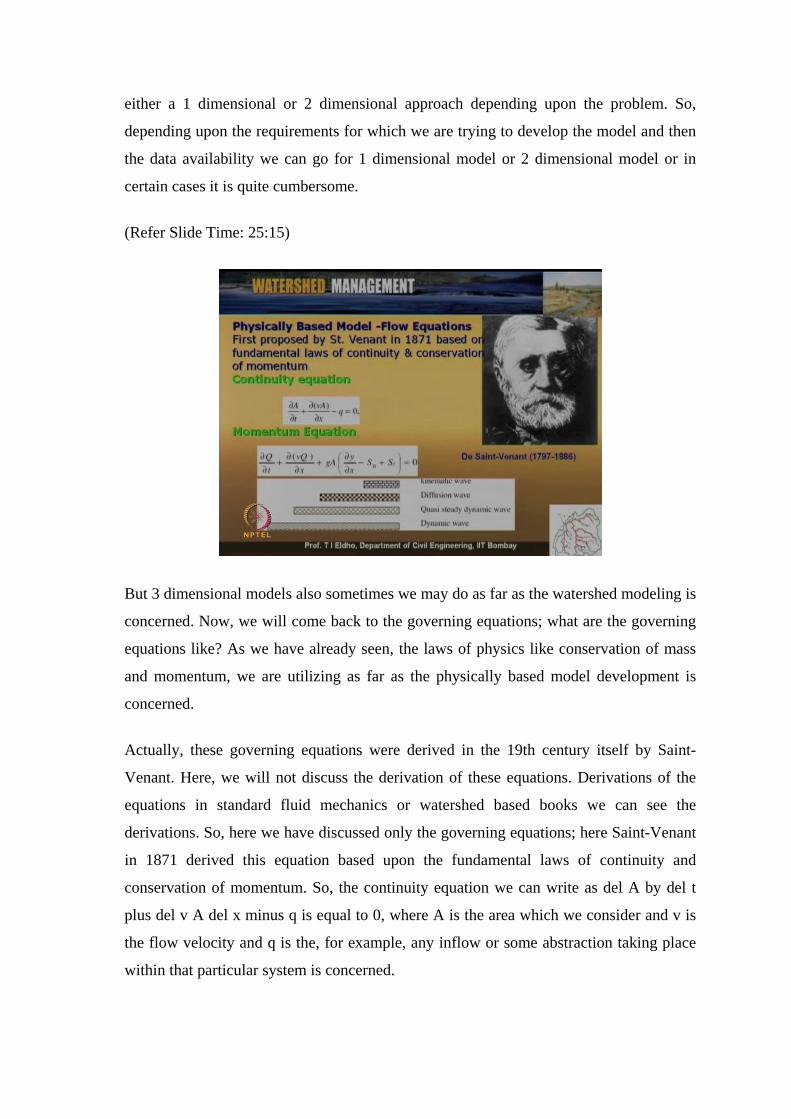
Actually, these governing equations were derived in the 19th century itself by Saint-
Venant. Here, we will not discuss the derivation of these equations. Derivations of the
equations in standard fluid mechanics or watershed based books we can see the
derivations. So, here we have discussed only the governing equations; here Saint-Venant
in 1871 derived this equation based upon the fundamental laws of continuity and
conservation of momentum. So, the continuity equation we can write as del A by del t
plus del v A del x minus q is equal to 0, where A is the area which we consider and v is
the flow velocity and q is the, for example, any inflow or some abstraction taking place
within that particular system is concerned.

Then this is the continuity equation and then momentum equation; we consider del Q by
del t plus del v Q by del x plus g A into del y by del x minus S 0 plus S f is equal to 0.
So, this is the momentum equation so here Q is the discharge at any particular location
which we consider then v is the flow velocity; then g is acceleration due to gravity A is
the area cross section or the flow of the section which we consider y is the depth of flow
S 0 is the bed slope S f is the energy slope. Now, these are the fundamental equations so-
called Saint-Venant’s equations a continuity equation momentum equations so when we
solve this so these equations you can see that this is presently it is given in 1 dimension
So if this is the watershed which we consider, if the main channel and then various
overland is concerned, we can consider as various strips or various plains joining to the
main channel and then it can be also considered overland flow; also can be considered 1
dimensional and the channel flow also can be considered as 1 dimensional. When we are
solving these both equations completely like the continuity and momentum equation
then, that kind of models are called dynamic wave modeling. So, this is the entire both
equations are considered then we call it as dynamic wave and then when we are not
considering the time dependent term in the momentum equation this term del Q by del t
then that kind of models are called Quasi study dynamic wave models. But, of course,
this will be solved with the continuity equation and then, when we are considering when
we are neglecting these two terms, only up to these terms are considered in the as the
momentum equation is concerned (Refer Slide Time: 28:35).
Then we call that kind of model diffusion wave model, this term in this equation and plus
the continuity equation, that is so-called diffusion wave modeling and the kinematic
wave model - a continuity equation and we consider this bed slope is equal to energy
slope so that kind of models are called kinematic wave model.

(Refer Slide Time: 28:45)
So, these physically based models we can classify into dynamic wave model Quasi
steady dynamic wave model or diffusion wave model and the kinematic wave models
this Saint-Venant’s - the equations divided by Saint-Venant’s are based upon certain
assumptions; the assumptions I have listed here. In this modeling in the governing
equations are based upon that the flow; is 1 dimensional then hydrostatic pressure
prevails and vertical accelerations are negligible then stream line curvature is small
bottom slope of the channel is small.
Steady uniform flow equation such as Manning’s or Chezy’s equation can be used to
describe the resistance effects or the frictional effects. Then, the fluid is incompressible;
so these equations are based upon these assumptions. So, the governing equation as I
mentioned in the previous slides, are 1 dimension nature as we can see that here if this is
the main channel for the watershed.

(Refer Slide Time: 29:48)
Then you can see that we consider as 1 dimensional flow and then the overland flow is
concerned, we consider strip flow joining the main channels as 1 dimension. If you
critically analyze the Saint-Venant’s equations, we can see that different forms of this
equations especially, momentum equations we can write in different forms. Say, either in
terms of velocity only or in terms of discharge only as shown in these two equations. So,
if you critically analyze this equation you can see that this term 1 by A del Q by del t or
del V by del t this is so-called local acceleration term and then this term which is V into
del V by del x or 1 by A del by del x of Q square by A; this is so-called convective
acceleration term.
Then this term is so-called pressure force term and then we are having the gravity force
term. So, here this S f is the frictional force term; as I mentioned, we can have a
kinematic wave form or diffusion wave form or dynamic wave form and if it steady state
we can have steady dynamic wave form also by neglecting the variations of this del V by
del t or this term. Local acceleration term can be neglected.
(Refer Slide Time: 30:01)
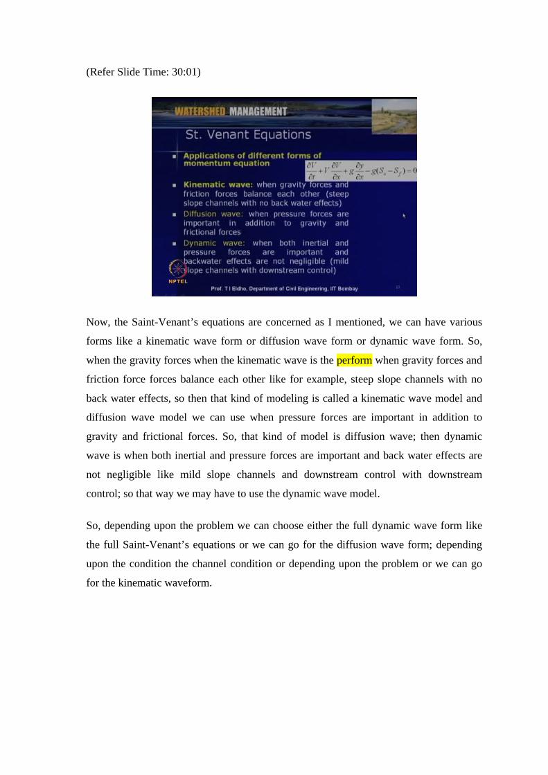
Now, the Saint-Venant’s equations are concerned as I mentioned, we can have various
forms like a kinematic wave form or diffusion wave form or dynamic wave form. So,
when the gravity forces when the kinematic wave is the perform when gravity forces and
friction force forces balance each other like for example, steep slope channels with no
back water effects, so then that kind of modeling is called a kinematic wave model and
diffusion wave model we can use when pressure forces are important in addition to
gravity and frictional forces. So, that kind of model is diffusion wave; then dynamic
wave is when both inertial and pressure forces are important and back water effects are
not negligible like mild slope channels and downstream control with downstream
control; so that way we may have to use the dynamic wave model.
So, depending upon the problem we can choose either the full dynamic wave form like
the full Saint-Venant’s equations or we can go for the diffusion wave form; depending
upon the condition the channel condition or depending upon the problem or we can go
for the kinematic waveform.

(Refer Slide Time: 32:25)
Accordingly, we can choose the model; so what we have discussed is the Saint-Venant’s
equations in its general form. As I mentioned, we are having the continuity equation
based upon the conservation of mass and then equation of motion based upon the
conservation of momentum. So as far as these equations are concerned, we can write
either in 2 dimensions or 1 dimension; most of the time either 2-D or 1-D equations will
be utilized. So, these equations different forms like conservative form or non
conservative form, different forms we can write depending upon the way which we
consider.
Now, we will consider this Saint-Venant’s equations for the overland flow and channel
flow separately; since when we go for watershed model as I mentioned, we may have to
consider the variation or the from the rainfall runoff with respect to the overland flow
and the channel flow. So, now let us see how we go for overland flow. The Saint-
Venant’s equation continuity equation in 2 dimension we can write in this form, where
del by del x of u bar h plus del by del y of w bar h plus del by del t of h is equal to r e
where r e is the rainfall excess so if r i is the rainfall then and f i is the infiltration and
taking place so r e we can get. The excess rainfall so this will be equal to r e; so where u
bar and v bar the velocity in x and y direction h is the depth of flow and x and y are the
dimensions in x direction y direction and t is the time.

So, then correspondingly as far as overland flow is concerned, the momentum equation 2
dimension we can write in this form: del u bar by del t plus u bar by into del u by del x
plus v bar del u by del y plus g del h by del x minus g into S o x minus S f x plus r e into
u bar by h is equal to 0; so here similarly we can write for the y component. So, u bar v
bar the velocity in x and y directions S o x and S o y are bed slope in x and y direction
and S f x and S f y the energy slope in x and y direction r e is the excess rainfall so this
way as far as overland flow.
(Refer Slide Time: 35:13)
Generally, overland flow we can consider as 2 dimension and but sometimes we can also
approximate as 1 dimension depending upon the way we are modeling; but, most of the
time channel flow we can consider as 1 dimension flow; so these are the governing
equations as far as the overland flow is concerned. Now, we have already seen now the
equations what we have seen is the dynamic wave form of the Saint-Venant’s equation.
So that, depending upon the condition we can simplify into diffusion waveform or
kinematic wave form. The diffusion wave form is shown here; so here the continuity
equation will be del q by del x plus del h by del t is equal to r e where q is the discharge
per unit width and r e is the rainfall excess.
So, this we can write with respect to the diffusion wave, the momentum equation will be
written as del h by del x is equal to S 0 minus S f where q is equal to u bar into h u bar is
the velocity in x direction and that is, can be written as alpha into h to the power beta
where alpha beta coefficients obtained from Manning’s equation. Beta can be written as
5 by 3 depending upon which wave consider then kinematic wave form. We can write as
del q by del x the continuity equation and the momentum equation continuity equation
saying del q by del x plus del h by del t is equal to r e and the momentum equation is just
bed slope is equal to energy slope.
For the dynamic wave form or the diffusion wave form or the kinematic wave form, now
the governing equations we have seen and now, to solve these equations we have to put
appropriate initial and boundary conditions. So, initial conditions, if you are going for
time dependent modeling initial conditions are required. Initial conditions can be either
we can assume the depth of flow throughout the watershed. We can assume as 0 or the
discharge can be assumed as 0 and then we can apply the boundary conditions. So,
boundary conditions can be, we know the upstream of the watershed like the ridge we
can assume the flow depth or the flow as equal to 0. The downstream condition we can
put the gradient of del h by del x or these kinds of gradient we can keep it as 0 or other
type of boundary conditions Dirichlet boundary conditions or the Neumann boundary
conditions can be applied. So, this either dynamic wave form or diffusion wave form or
the kinematic wave form as far as the overland flow is concerned, we can solve these
governing equations by using a numerical technique.
You can see that the governing equations partial differential equations; we have to go for
numerical solutions as far as the solution is concerned, like a finite difference method or
finite terminal method. So, we have to solve these governing equations and apply the
suitable initial and boundary conditions for the concerned watershed and then we can
develop the model to obtain the runoff at the particular locations for the watershed is
concerned. Here, like many other losses like evapotranspiration or the infiltration all
these losses we can account as far as the rainfall excess calculation is concerned; so
accordingly we can deal with the model.
(Refer Slide Time: 38:52)
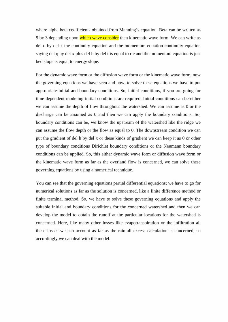
So, now so that is about the overland flow. Now, coming back to the channel flow, the
other component is the channel flow. So, this overland flow will be joining to the
channel at the particular locations. so you can see that if this is the watershed and then if
this is your main channel, so then the when the rainfall takes place the runoff will be
coming from the channel overland and will be joining to the channel and then we have to
route the flow through the channel depending upon the wave changes taking place with
respect to the overland flow component. Here, the governing equations are the Saint-
Venant’s equation but we can write slightly in a different way. The equation of
continuity is del Q by del x plus del A by del t minus q is equal to 0, where Q is the
discharge in the channel, A is the area flow in the channel and q is the lateral inflow
coming to the channel as overland flow.
The momentum equation can be written as del Q by del t plus del by del x of Q square by
A is equal to g into A into S 0 minus S f minus g into A into del h by del x. so, this as I
mentioned, this momentum equation different forms we can have; so one particular form
is mentioned here.
So, here this energy slope S f we can use Manning’s equation or Chezy’s equation to get
those values and then we can solve this equation. Simultaneously, so that with respect to
the overland flow from various locations we can route the flow and then identify what
will be the discharge versus time at any particular location of the channel or the outlet of

the watershed. So, that way the channel flow equations are solved. Here, also we need to
go for numerical techniques like a finite difference or finite element modeling to solve
these equations and then use the appropriate initial and boundary conditions. So, here
also initial conditions like depth of flow in the channel or the discharge through the
channel can be initial conditions at the beginning and then the boundary conditions can
be at the outlet or at the beginning of the channel. What should be the flow coming? Or,
if the channel is starting at the beginning of the watershed then that can be 0 depth.
(Refer Slide Time: 41:01)
Then now similar to overland flow here also channel flow is also concerned, we can have
the diffusion wave model and kinematic wave model. So, in diffusion wave model the
governing equation is del Q by del x plus del A by del t minus Q is equal to 0 the
continuity equation and the momentum equation is the simplified as del h by del x is
equal to S 0 minus S f. So, this S f we can use the Manning’s equation or other Chezy’s
equation and then in kinematic approach the continuity equation is same and then we
assume the energy slope is equal to bed slope. Here also, we apply the initial conditions
and the boundary conditions to identify how the flow pattern is taking place.
How the discharge versus time or depth versus time? We can identify by solving this
system of equations; by using numerical techniques. So, either dynamic wave form or the
diffusion wave form or the kinematic wave form; we have seen the governing equations
and now using this governing equation, using particular numerical models and we can

solve the system of equations. Then apply the boundary conditions initial conditions and
boundary conditions and then the output will be the depth of flow or the discharge at any
location of the channel. Now, we have seen the overland flow and the channel flow. If
you want to identify the runoff process taking place within the watershed then we have to
couple this overland flow model and channel flow model and then we have to see the
coupled we have to run the coupled model. By applying suitable boundary conditions for
the watershed, these numerical modeling issues we will discuss in the next lecture and
then the coupling aspect also.
(Refer Slide Time: 43:01)
Now, the use of numerical simulation models: as I mentioned, this governing equation
we have to solve using numerical techniques. So, hydrologic simulation models use
mathematical equations as we have seen in the previous slides to calculate the results like
runoff volume or the peak flow. Then, computer models allow parameters variation in
space and time with use of numerical methods. So, like finite difference, finite element
or method of characteristics or finite volume methods. Then, the ease in simulation of
complex rainfall pattern and heterogeneous watershed depending upon what kind of
either semi distributed or distributed or what kind of numerical approach we use. Then,
evaluation of various design controls and schemes; like, if there are various hydraulic
structures how to deal with those structures and how to deal with the various parameters
variations like that?

Then effective use of land use and land cover parameters. so for the given watershed the
land use land cover will be varying. So, then accordingly, the for example, Manning’s
reference coefficient will be varying in the overland flow modeling or various
parameters like ferocity saturated hydrologic conductivity, etcetera, will vary so that we
can identify and then the spatial characteristics variation if we can take care.
Then we can have better quality or better models for the runoff model for the given
rainfall conditions. Now, before closing this lecture let us see some of the classifications
of the models. So, like we have seen now the modeling is based upon the Saint-Venant’s
equation or its variations.
(Refer Slide Time: 44:47)
Some of the examples hydrodynamic and empirical models I have listed here. So, the
physical processes are listed here then the hydrodynamic models and some of the
empirical models for example, if we are dealing with surface runoff we can have the
dynamic wave model or the its variations like diffusion wave model or kinematic wave
model. Then simple conceptual models like mass balance approach models. So, various
models are there some of the important models are only listed here and then empirical
equations like rational method or unit hydrograph method, or lumped model like SCS
method we can have it.
Then infiltration is concerned we can have various forms of the infiltration empirical
equations or the solution to Richards equations or Green-Ampt equation or Philip-two
term equations or simplified form of kinematic form. Then the empirical types
infiltration models like a SCS method we can also calculate based upon SCS-CN or
some kinds of algebraic variations or HEC models.
Then groundwater variation is concerned like base flow; then model based upon ground
water flow equations which we will be discussing in coming lectures and then algebraic
equations like Horton equation based upon that or evapotranspiration’s like as we have
already seen, various equations we can utilize like a Penman-Monetelith equation or
Morten method or Blaney Criddle method like that.
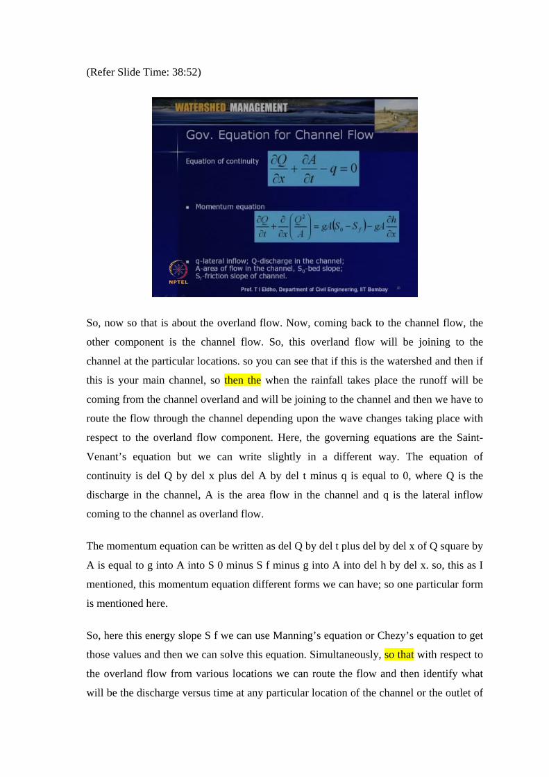
(Refer Slide Time: 46:22)
Then flow over porous bed is concerned we can either go for kinematic wave dynamic
wave or volume balance models, or then empirical like SCS model, then flow in channel
is concerned, as we discussed kinematic diffusion or dynamic hydrodynamic models or
Muskingum method or hydrograph analysis. Then, the solute transport is concerned
within the watershed model based upon advection-dispersion or Fickian models. We can
have, so these issues also we discuss later; or we can have some algebraic type of
modeling. Then, sediment transport is concerned we can go for diffusion - dynamic or
kinematic or Einstein bed load based equations or Sediment graph models or Regression
equations.
So, like that if we go through the hydrologic literature large number of models we can
see; may be some of the authors mentioned may be 1000’s of models have been
developed for the last few decades depending upon the conditions depending upon the
assumptions or various variation like 1-D, 2-D or 3 dimensions or how many parameters
we consider or what kind of hydrologic process are concerned.
So, accordingly we can see that there are number of hydrodynamic and empirical models
available in literature. You can choose particular model depending upon your
requirement your objectives and then we can solve the particular problem as per the
objectives.
(Refer Slide Time: 47:59)
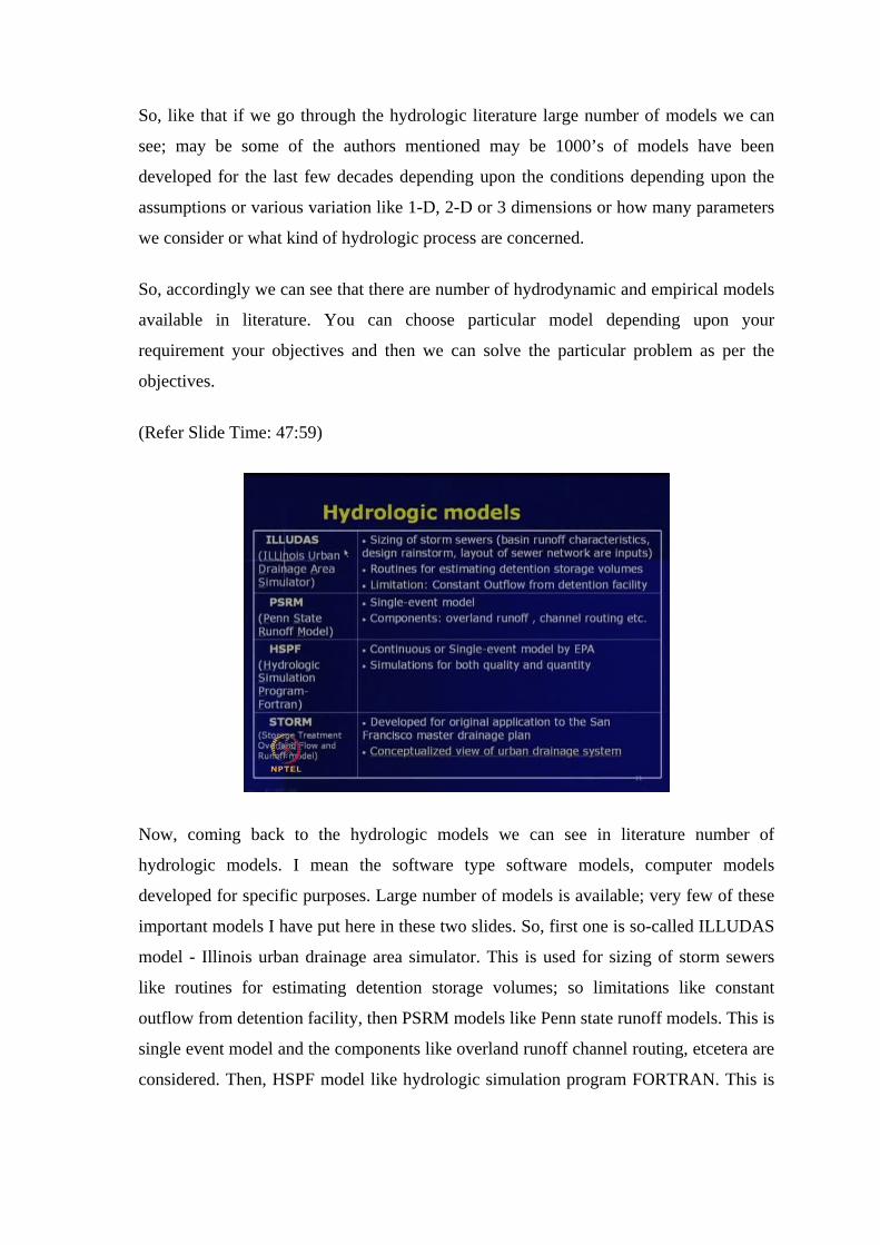
Now, coming back to the hydrologic models we can see in literature number of
hydrologic models. I mean the software type software models, computer models
developed for specific purposes. Large number of models is available; very few of these
important models I have put here in these two slides. So, first one is so-called ILLUDAS
model - Illinois urban drainage area simulator. This is used for sizing of storm sewers
like routines for estimating detention storage volumes; so limitations like constant
outflow from detention facility, then PSRM models like Penn state runoff models. This is
single event model and the components like overland runoff channel routing, etcetera are
considered. Then, HSPF model like hydrologic simulation program FORTRAN. This is

either it can be continuous or single event based or simulation for both quality and water
quality and quantity can be considered.
(Refer Slide Time: 49:03)
Then storm model: like developed for original application to the San Francisco master
drainage plan. So, this is based upon conceptualized view of urban drainage systems and
then we can have a SWMM model storm water management model. There are routings
for surface subsurface or groundwater components. Then this can fully dynamic
hydraulic flow routing then, we can have HEC series or HECHMS models. So, it can be
either DOS based or windows, based then these models can be used to calculate runoff
hydrograph at each component like channels. Then, various locations, etcetera; then
WMS watershed modeling system... these provide the link to various available model
using the GIS package and hydrologic models so including like HECTR-55 TR-20 there
are links to this various model in the watershed modeling systems.
Then IHACRES: this is a particular model simulation of stream flow from basins of
various sizes unit hydrograph approach to lumped modeling. So, if you go through the
hydrologic literature, you can see number of models like this. As I mentioned, depending
upon the requirement, depending upon the objectives, you can choose particular model
or you can develop your model also depending upon your requirement.

(Refer Slide Time: 50:16)
So, now finally, what are the important steps in watershed simulation analysis? When we
are going for watershed simulation and the steps include, so first we can choose the
model depending upon the objectives or the requirement and data availability, then we
have to collect the data input data collection: like rainfall infiltration, physiography, land
use channel characteristics, etcetera. Then we can evaluate the study objectives under
various watershed simulation conditions. So, we can see various scenarios and then
accordingly, we can simulate then selection of methods for obtaining basin hydrographs
and channel routing as far as hydrology is concerned for the given rainfall condition or
the given intensity of the possible rainfall how the system will be behaving.
Then we have to do calibration and verification of the models as we discussed earlier;
then model simulation for various conditions for example, if a dam is built of this
particular height what will happen? How much is the storage possible? so like that
various conditions we can simulate and then various parameter sensitivity also we can
carry out.

(Refer Slide Time: 51:33)
Then we can evaluate the usefulness of model and then comment on the needed changes.
As far as the watershed modeling is concerned, these are some of the important steps in
watershed simulation analysis. Now, before closing this lecture, here two examples: one
is distributed model based upon the kinematic wave approach; so here the kinematic
equations we have already seen. Here, we consider an area of this for overland flow 400
meter by 500 meter size area, then slope S 0 is given as 0.0005; Manning’s coefficient is
0.02 and we apply uniform excess rainfall r is equal to 0.33 mm per minute and duration
is 200 minutes. So this is the area we consider; we have to identify, how much is the
runoff taking place with respect to time for this overland area. For this actually, Jaber
and Mohtar in their paper in 2003 have given they have given the analytical solutions so
the solution is given by this equation.
So, I am not going the details of this equation; so this q represent the discharge of flow
per unit width and so then alpha and beta, some of the coefficient and here tc is the time
of concentration, tr is the rainfall duration, tf is the simulation time. And, this also we
have done - the overland flow simulation by using finite element model which we will be
discussing in the next lecture. So, we run the model and then we simulated by using the
kinematic wave approach and then its corresponding analytical solution; also you can see
here with respect to time how the discharge variation is given here.

This line represents the analytical solution and then the kinematic wave model results for
2 time stamp; one is 30 second and another one is 80 second. We can see that there is a
good match for the analytical solution of the kinematic wave model but, we can see that
this analytical solution we can apply only for very simple cases like this. But, for a field
case we cannot have these kinds of analytical solution but, since we developed a model
based upon finite element method for the solution of the kinematic wave approach, we
used this analytical solution for verification of the developed model. So, the
corresponding finite element formulation we will be discussing in the next lecture.
(Refer Slide Time: 54:01)
Then, another application to a case study area called Banaha watershed. As I mentioned
in a civil department IIT Bombay, we have developed some watershed models based
upon the kinematic wave approach and diffusion wave approach using the finite element
method. So, that models we have applied for watershed called Banaha watershed. The
modeling details we will discuss in the next lecture but, here my purpose is to discuss the
variation, the physically based model application to identify how the runoff is taking
place for the given rainfall condition.
So here the watershed is located in Chatra district in Jharkhand state and area is 16.72
square kilometer and major soil class is sandy loam and here we use a remote sensing
data and GIS is used for drainage slope and LULC maps. Then, Manning’s roughness all
these details we obtained from the using the arc GIS and so, mean value of slope and

Manning’s roughness for each grid is assigned and then accordingly the variation is
taken.
(Refer Slide Time: 55:21)
So this is the watershed and this is the main channel; this is the outlet of the channel; so,
this shows actually we developed a digital elevation model for this watershed and this is
showing the elevation variation for the watershed. So, here this is the variation with
respect to the watershed. Then here, this shows the slope variation and this shows the
land use variation for the watershed. So, this is the grid which we utilized using the finite
element method this is this is the 1 dimensional modeling approach.
(Refer Slide Time: 56:05)
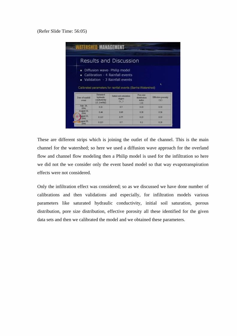
These are different strips which is joining the outlet of the channel. This is the main
channel for the watershed; so here we used a diffusion wave approach for the overland
flow and channel flow modeling then a Philip model is used for the infiltration so here
we did not the we consider only the event based model so that way evapotranspiration
effects were not considered.
Only the infiltration effect was considered; so as we discussed we have done number of
calibrations and then validations and especially, for infiltration models various
parameters like saturated hydraulic conductivity, initial soil saturation, porous
distribution, pore size distribution, effective porosity all these identified for the given
data sets and then we calibrated the model and we obtained these parameters.
(Refer Slide Time: 56:52)
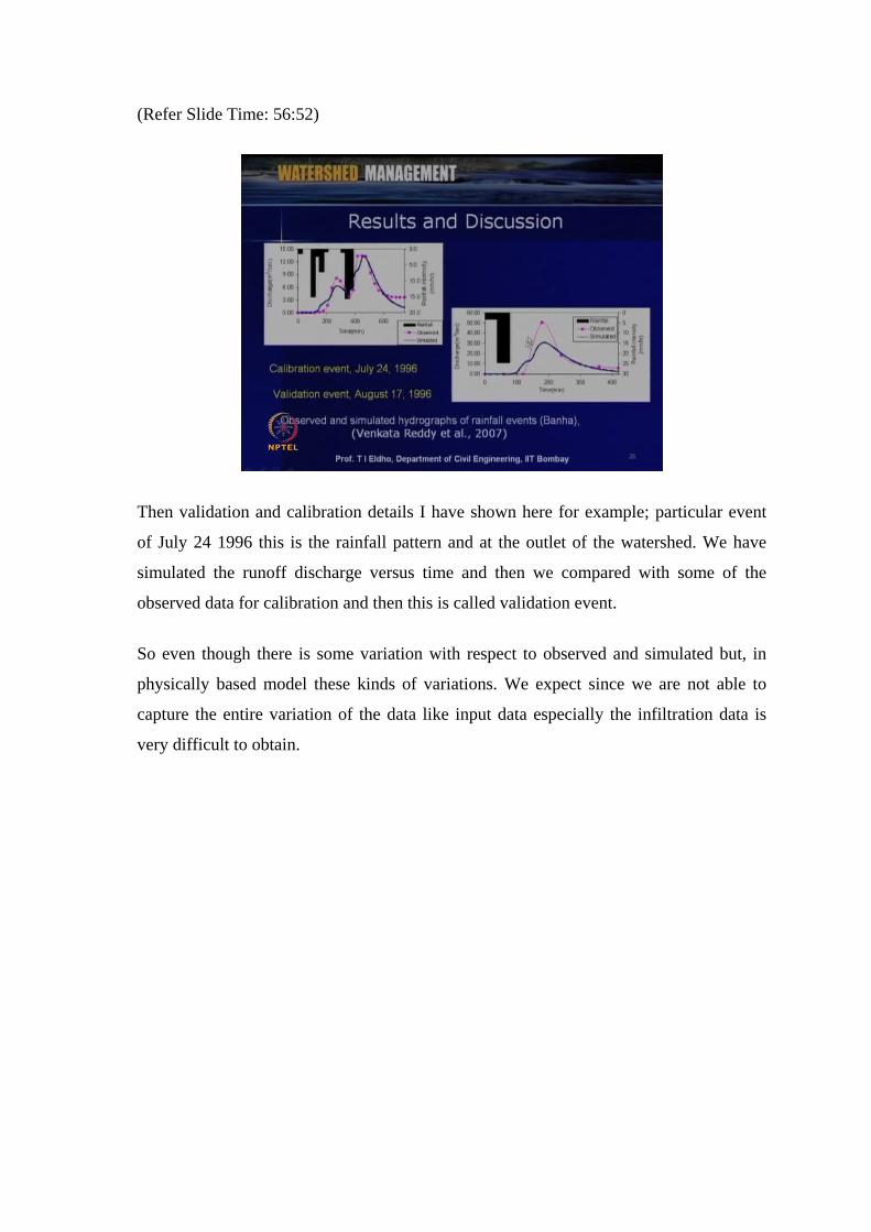
Then validation and calibration details I have shown here for example; particular event
of July 24 1996 this is the rainfall pattern and at the outlet of the watershed. We have
simulated the runoff discharge versus time and then we compared with some of the
observed data for calibration and then this is called validation event.
So even though there is some variation with respect to observed and simulated but, in
physically based model these kinds of variations. We expect since we are not able to
capture the entire variation of the data like input data especially the infiltration data is
very difficult to obtain.
(Refer Slide Time: 57:41)
So that way; some of the parameters we started with the literature values and then we
tried to calibrate and those parameters were used for the modeling. Now, these are some
of the important references which were used in today’s lecture; so like this paper which
you published in the hydrological process.
(Refer Slide Time: 57:52)
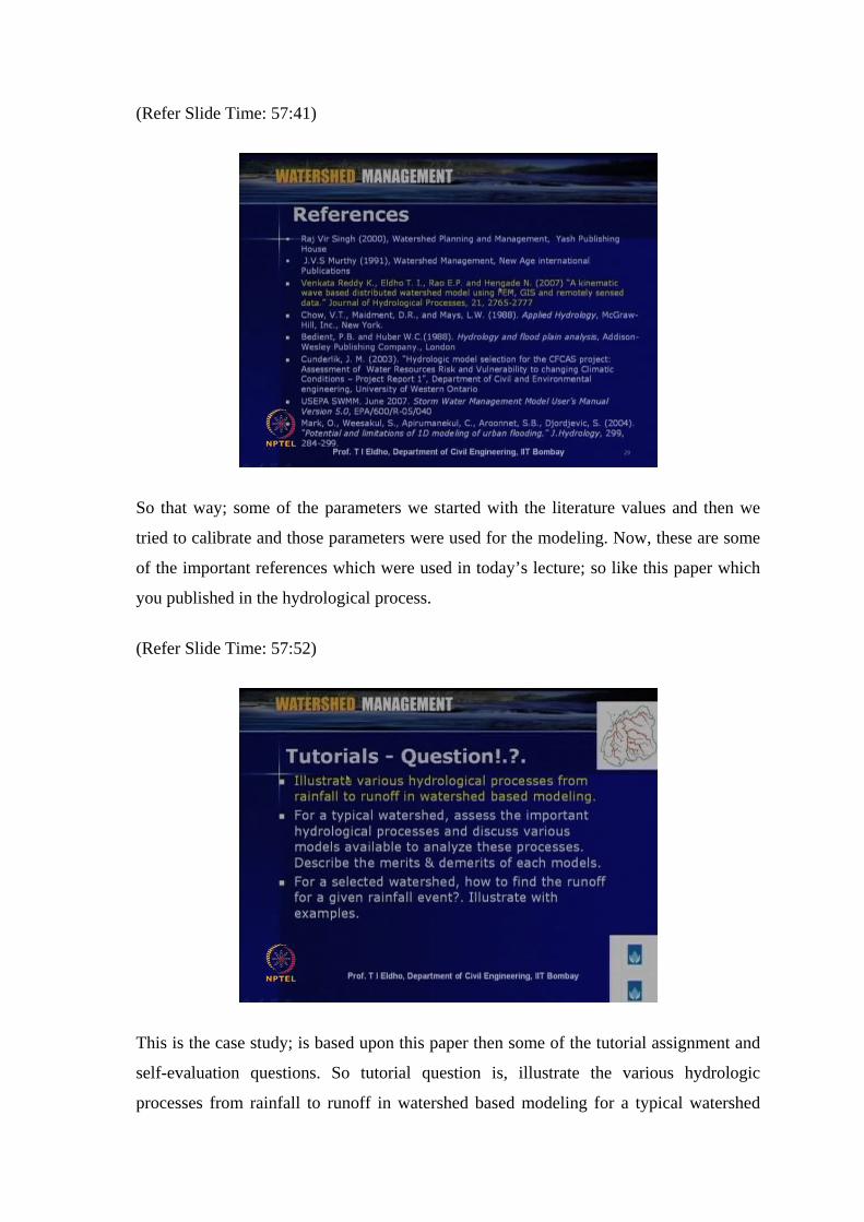
This is the case study; is based upon this paper then some of the tutorial assignment and
self-evaluation questions. So tutorial question is, illustrate the various hydrologic
processes from rainfall to runoff in watershed based modeling for a typical watershed

assess the important hydrological processes and discuss various models available to
analyze these processes.
(Refer Slide Time: 58:27)
Describe the merits and demerits of each models for a selected watershed how to find the
runoff for a given rainfall event illustrate with examples so these details are based upon
today’s lecture so you can easily get the solution then self-evaluation questions describe
different categories of deterministic hydrologic models.
What is the importance of physically based watershed modeling and describe the Saint-
Venant’s equations with its applications assumptions and importance compared the
following lumped semi distributed and distributed models HEC-HMS SWMM MIKE-11
models.

(Refer Slide Time: 58:55)
Discuss the applications advantages/disadvantages of each model; few assignment
questions differentiate between lumped semi-distributed and distributed models used in
hydrologic modeling and how physically based watershed modeling is done.
Illustrate the step by step procedure; what are the advantages and limitations? What are
the important steps in the watershed simulation analysis illustrate various types of
hydrodynamic and empirical models used in hydrology.
(Refer Slide Time: 59:23)

So, all these questions you can answer based upon today’s lecture finally one unsolved
problem for your watershed area discuss the possibility of applying a physically based
model for a runoff or flood analysis identify the data required for physical modeling
develop a conceptual model by giving the detailed steps for rainfall runoff modeling.
Then identify how to model evapotranspiration interception infiltration for the area
considered with respect to available data. Choose specific models to model these
processes; discuss how to add these processes in the rainfall runoff modeling. Based
upon today’s lecture and the previous lectures, you can easily do this unsolved problem.
So, now, today we discussed the hydrologic modeling based upon the physically based
approach now in the next lecture. We will discuss some of the numerical tools. How to
solve these kinds of Saint-Venant’s equations or its variations and then we will discuss
some more case studies; thank you.