lec 11: response surface methodologygauss.stat.su.se/gu/ep/lec11.pdfying li lec 11: response surface...
TRANSCRIPT

Lec 11: Response Surface Methodology
Ying Li
December 6, 2011
Ying Li Lec 11: Response Surface Methodology
Response Surface Methodology (RSM)
A collection of mathematical and statistical techniques;
Model and analysis of problems in which a response ofinterest;
The objective is to optimize the response.
Ying Li Lec 11: Response Surface Methodology

Ying Li Lec 11: Response Surface Methodology

RSM is a sequential procedure
Factor screening
Finding the regionof the optimum
Modeling &Optimization of theresponse
Ying Li Lec 11: Response Surface Methodology

Response Surface Models
Screening:
y = β0 + β1x1 + β2x2 + β12x1x2 + ε
Steepest ascent:
y = β0 + β1x1 + β2x2 + ε
Optimization
y = β0 + β1x1 + β2x2 + β12x1x2 + β11x21 + β22x
22 + ε
Ying Li Lec 11: Response Surface Methodology

Steepest Ascent
A procedure for movingsequentially from aninitial “guess” towards toregion of the optimum.
Based on the fittedfirst-order model
y = β0 + β1x1 + β2x2
Ying Li Lec 11: Response Surface Methodology

An Example of Steepest Ascent
A chemical engineer is interested in determining the operatingconditions that maximize the yield of a process. Two controllablevariables: reaction time (ξ1) and reaction temperature (ξ2).
Ying Li Lec 11: Response Surface Methodology

A first-order model may be fit to these data by least squares.
y = 40.44 + 0.775x1 + 0.325x2
Ying Li Lec 11: Response Surface Methodology

Ying Li Lec 11: Response Surface Methodology

Ying Li Lec 11: Response Surface Methodology

Summary of steepest ascent
Points on the path of steepest ascent are proportional to themagnitudes of the model regression coefficients.
The direction depends on the sign of the regression coefficient.
Ying Li Lec 11: Response Surface Methodology
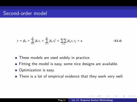
Second-order model
These models are used widely in practice.
Fitting the model is easy, some nice designs are available.
Optimization is easy.
There is a lot of empirical evidence that they work very well.
Ying Li Lec 11: Response Surface Methodology

General solution for second-order model
y = β0 + x′b + x′Bx
Ying Li Lec 11: Response Surface Methodology

The stationary point
∂y
∂x= b + 2Bx = 0
xs = −1
2B−1b⇐ the stationary point
ys = β0 +1
2x′sb
Ying Li Lec 11: Response Surface Methodology
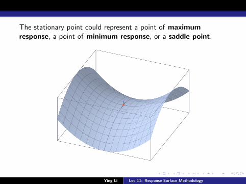
The stationary point could represent a point of maximumresponse, a point of minimum response, or a saddle point.
Ying Li Lec 11: Response Surface Methodology

Canonical Analysis
xs = −1
2B−1b ys = β0+
1
2x′sb
The canonical form:
y = ys +λ1ω21+λ2ω
22+·+λkω2
k
the {λi} are the eigenvalues orcharacteristic roots of thematrix B
Ying Li Lec 11: Response Surface Methodology

Canonical Analysis
The nature of the response surface can be determined from thestationary point & the signs and magnitudes of the {λi}.
all positive: a minimum is found
all negative: a maximum is found
mixed: a saddle point is found
The response surface is steepest in the direction (canonical)corresponding to the largest absolute eigenvalue
Ying Li Lec 11: Response Surface Methodology

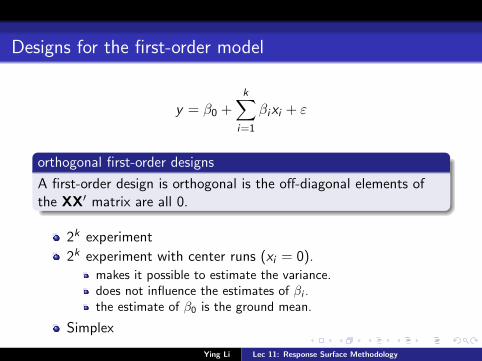
Designs for the first-order model
y = β0 +k∑
i=1
βixi + ε
orthogonal first-order designs
A first-order design is orthogonal is the off-diagonal elements ofthe XX′ matrix are all 0.
2k experiment
2k experiment with center runs (xi = 0).makes it possible to estimate the variance.does not influence the estimates of βi .the estimate of β0 is the ground mean.
Simplex
Ying Li Lec 11: Response Surface Methodology

Simplex
Simplex: a regularly sided figure with k + 1 vertices in kdimensions.
Figure: The simplex design for k = 2 and k = 3 variables
Ying Li Lec 11: Response Surface Methodology

Designs for the second order model
Central composite design
Box-Behnken design
Face-centered design
Equiradial design
small composite design & hybrid design
Ying Li Lec 11: Response Surface Methodology

Central composite design
The CCD consists of a 2k factorial with nF factorial runs, 2k axialor star runs, and nc center runs.
Two parameters in such design: the distance α of the axial runsfrom the center; the number of the center points nc
Ying Li Lec 11: Response Surface Methodology

Rotatability
Rotatable
A second-order response surface design is rotatable if the varianceof the predicted response V [y(x)] is the same at all the points of xthat are at the same distance form the design center: α = (nF )1/4
Ying Li Lec 11: Response Surface Methodology

Rotatability
A rotatable design gives the same prediction in all directions.
Ying Li Lec 11: Response Surface Methodology

Rotatability
A rotatable design gives the same prediction in all directions.
Ying Li Lec 11: Response Surface Methodology

Spherical CCD
All factorial runs and axial runs have the same distance to thecenter: α = (k)1/2
Figure: The distance α between the axial points and the center
Ying Li Lec 11: Response Surface Methodology

Spherical CCD
All factorial runs and axial runs have the same distance to thecenter: α = (k)1/2
Figure: The distance α between the axial points and the center
Ying Li Lec 11: Response Surface Methodology

Box-Behnken Design
Three-level designs for small number of runs.
All points are on the distance 21/2 = 0.707 from the center.
No points at the vertices.
Either rotatable or nearly rotatable.
Ying Li Lec 11: Response Surface Methodology

Face-centered cube
The axial points are on the surface of the cube (α = 1).
Conveniently, because it only use three levels per factor.
Not rotatable.
Ying Li Lec 11: Response Surface Methodology
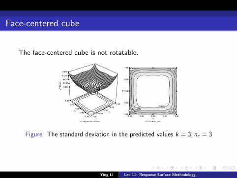
Face-centered cube
The face-centered cube is not rotatable.
Figure: The standard deviation in the predicted values k = 3, nc = 3
Ying Li Lec 11: Response Surface Methodology

Equiradial design
Design for two variables
Rotatable
Ying Li Lec 11: Response Surface Methodology

Graphical Evaluation of Response Surface Designs
Scaled prediction variance (SPV):
NV [y(x)]
σ2= Nx ′(X ′X )−1x
The variance dispersion graph (VDG) plot the maximum, theminimum and the average scaled prediction variance against thedistance to the center.
Ying Li Lec 11: Response Surface Methodology

Variance dispersion graph
a Rotatable CCDfor k = 3(nc = 4,α = 1.68)
b Spherical CCDfor k = 3(nc = 4,α = 1.73)
Ying Li Lec 11: Response Surface Methodology
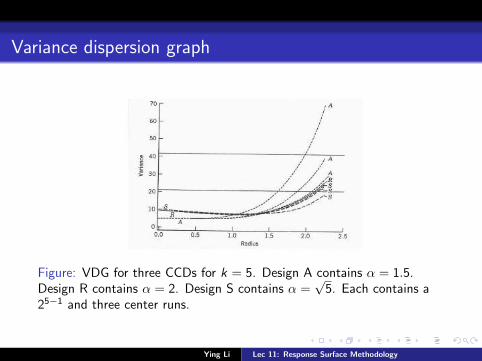
Variance dispersion graph
Figure: VDG for three CCDs for k = 5. Design A contains α = 1.5.Design R contains α = 2. Design S contains α =
√5. Each contains a
25−1 and three center runs.
Ying Li Lec 11: Response Surface Methodology

Variance dispersion graph
Figure: VDG for three CCDs for k = 5. Design A contains α = 1.5.Design R contains α = 2. Design S contains α =
√5. Each contains a
25−1 and three center runs.
Ying Li Lec 11: Response Surface Methodology

Variance dispersion graph
Figure: for central composite design for k = 4 and α = 2. Four or fivecentral point (nc = 4or5) gives a stable variance in the predicted values.
Ying Li Lec 11: Response Surface Methodology

Design criteria
D-optimal design for minimizing the variance of the modelregression coefficients.min |(X ′X )−1|G-optimal design for minimizing the maximum predictionvariance. min maxVar(y)
I-optimal design for its smallest possible value of the averageprediction variance. min averageVar(y)
Ying Li Lec 11: Response Surface Methodology
Which Criterion Should I Use?
For fitting a first-order model, D is a good choice
Focus on estimating parametersUseful in screening
For fitting a second-order model, I is a good choice
Focus on response predictionAppropriate for optimization
Ying Li Lec 11: Response Surface Methodology