Least-Squares Finite Element Methods for

Quantum Electrodynamics

by

Christian W. Ketelsen

B.S., Washington State University, 2003

M.S., Washington State University, 2005

A thesis submitted to the

Faculty of the Graduate School of the

University of Colorado in partial fulfillment

of the requirements for the degree of

Doctor of Philosophy

Department of Applied Mathematics

2010

This thesis entitled:Least-Squares Finite Element Methods for Quantum Electrodynamics

written by Christian W. Ketelsenhas been approved for the Department of Applied Mathematics

Prof. Thomas A. Manteuffel

Prof. Stephen F. McCormick

Date

The final copy of this thesis has been examined by the signatories, and we find thatboth the content and the form meet acceptable presentation standards of scholarly

work in the above mentioned discipline.

iii

Ketelsen, Christian W. (Ph.D., Applied Mathematics)

Least-Squares Finite Element Methods for Quantum Electrodynamics

Thesis directed by Prof. Thomas A. Manteuffel

The numerical solution of the Dirac equation is the main computational bottle-

neck in the simulation of quantum electrodynamics (QED) and quantum chromodynam-

ics (QCD). The Dirac equation is a first-order system of partial differential equations

coupled with a random background gauge field. Traditional finite-difference discretiza-

tions of this system are sparse and highly structured, but contain random complex

entries introduced by the background field. For even mildly disordered gauge fields the

near kernel components of the system are highly oscillatory, rendering standard multi-

level iterative methods ineffective. As such, the solution of such systems accounts for

the vast majority of computation in the simulation of the theory.

In this thesis, two discretizations of a simplified model problem are introduced,

based on least-squares finite elements. The first discretization is obtained by direct

discretization of the governing equation using least-squares finite elements. The second

is obtained by applying the same discretization methodology to a transformed version of

the original system. It is demonstrated that the resulting linear systems satisfy several

desirable physical properties of the continuum theory and agree spectrally with the

continuum the operator. To date, these are the first discretizations to accomplish these

goals without extending the theory to a costly extra dimension.

Finally, it is shown that the resulting linear systems are amenable to effective pre-

conditioning by algebraic multigrid methods. Specifically, classical algebraic multigrid

(AMG) and adaptive smoothed aggregation (αSA) multigrid are employed. The result

is a solution process that is efficient and scalable as both the lattice size and the disorder

of the background field is increased, and the simulated fermion mass is decreased.

Dedication

To Mom and Dad.

v

Acknowledgements

This work was influenced by a great number of people. First and foremost, I want

to thank my advisors, Tom Manteuffel and Steve McCormick. From them I learned how

to be a better researcher, teacher, and professional. They taught me that sometimes you

have to play hard before you can work hard, and that often times the best mathematics

is done on a bicycle, a mountain top, or a ski lift. This work would not have been

possible without the help of John Ruge and Marian Brezina. Their patience with my

programming ineptitude was the stuff of legends. In addition, I must thank the entire

Grandview Gang: James Adler, Eunjung Lee, Josh Nolting, Minho Park, Geoff Sanders,

and Lei Tang. Without them, the pun-ishment of Tuesday marathon meetings would

surely have been unbearable. I also need to thank every physicist that I ever bugged

with endless conceptual questions. James Brannick, Rich Brower, Mike Clark, Tom

DeGrand, Anna Hasenfratz, Claudio Rebbi, and Pavlos Vranas each provided lifesaving

insight at some time in the course of this work. I must also thank Markus Berndt and

Dave Moulton of Los Alamos National Laboratory for putting up with me for three

summers. Many of the ideas in this thesis were born in the sweltering heat of a cubicle

at 7300 feet. Finally, I want to thank my family and the rest of my Boulder friends for

their endless support during the last four years. They kept me mostly sane.

vi

Contents

Chapter

1 Introduction 1

2 The Continuum Model 6

2.1 Continuum Dirac Operator . . . . . . . . . . . . . . . . . . . . . . . . . 6

2.2 The Schwinger Model . . . . . . . . . . . . . . . . . . . . . . . . . . . . 11

2.2.1 Gauge Covariance . . . . . . . . . . . . . . . . . . . . . . . . . . 12

2.2.2 Chiral Symmetry . . . . . . . . . . . . . . . . . . . . . . . . . . . 16

2.2.3 An Alternate Formulation . . . . . . . . . . . . . . . . . . . . . . 18

3 The Discrete Model 22

3.1 The Naive Discretization . . . . . . . . . . . . . . . . . . . . . . . . . . . 23

3.1.1 Gauge Covariance . . . . . . . . . . . . . . . . . . . . . . . . . . 25

3.1.2 Chiral Symmetry . . . . . . . . . . . . . . . . . . . . . . . . . . . 27

3.1.3 Species Doubling . . . . . . . . . . . . . . . . . . . . . . . . . . . 29

3.2 Wilson’s Discretization . . . . . . . . . . . . . . . . . . . . . . . . . . . . 31

4 The Least-Squares Finite Element Method 36

5 Least-Squares Finite Elements for the Schwinger Model 40

5.1 The Least-Squares Discretization . . . . . . . . . . . . . . . . . . . . . . 41

5.1.1 Gauge Covariance . . . . . . . . . . . . . . . . . . . . . . . . . . 51

vii

5.1.2 Chiral Symmetry . . . . . . . . . . . . . . . . . . . . . . . . . . . 62

5.1.3 Species Doubling . . . . . . . . . . . . . . . . . . . . . . . . . . . 64

5.2 H1-Ellipticity . . . . . . . . . . . . . . . . . . . . . . . . . . . . . . . . . 67

5.2.1 Main Theorem . . . . . . . . . . . . . . . . . . . . . . . . . . . . 68

5.2.2 Implications . . . . . . . . . . . . . . . . . . . . . . . . . . . . . . 85

5.3 Numerical Experiments . . . . . . . . . . . . . . . . . . . . . . . . . . . 87

5.3.1 Multigrid Methods . . . . . . . . . . . . . . . . . . . . . . . . . . 87

5.3.2 Numerical Results . . . . . . . . . . . . . . . . . . . . . . . . . . 95

6 Least-Squares Finite Elements for a Transformed Schwinger Model 101

6.1 Discretization of the Transformed System . . . . . . . . . . . . . . . . . 101

6.1.1 Gauge Covariance . . . . . . . . . . . . . . . . . . . . . . . . . . 105

6.1.2 Chiral Symmetry . . . . . . . . . . . . . . . . . . . . . . . . . . . 110

6.1.3 Species Doubling . . . . . . . . . . . . . . . . . . . . . . . . . . . 113

6.2 H1-Ellipticity . . . . . . . . . . . . . . . . . . . . . . . . . . . . . . . . . 113

6.2.1 Main Theorem . . . . . . . . . . . . . . . . . . . . . . . . . . . . 114

6.3 Numerical Experiments . . . . . . . . . . . . . . . . . . . . . . . . . . . 115

6.3.1 Numerical Results . . . . . . . . . . . . . . . . . . . . . . . . . . 115

7 Conclusions and Future Work 121

Bibliography 125

viii

Tables

Table

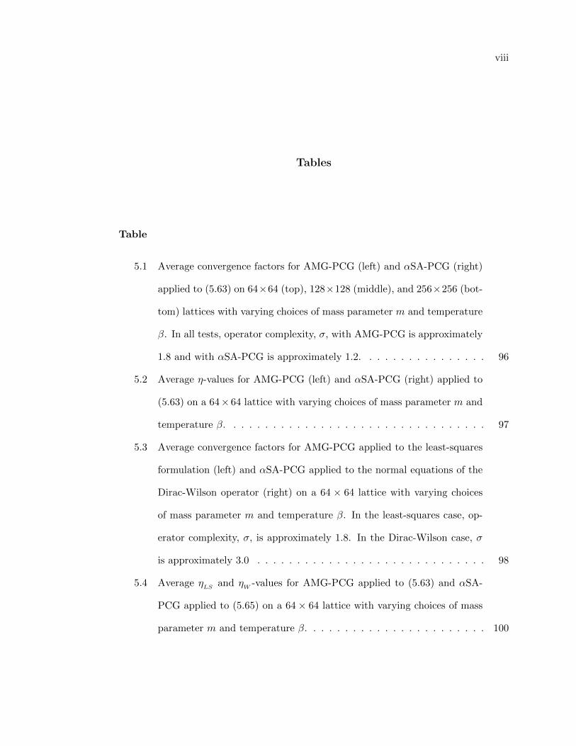
5.1 Average convergence factors for AMG-PCG (left) and αSA-PCG (right)

applied to (5.63) on 64×64 (top), 128×128 (middle), and 256×256 (bot-

tom) lattices with varying choices of mass parameter m and temperature

β. In all tests, operator complexity, σ, with AMG-PCG is approximately

1.8 and with αSA-PCG is approximately 1.2. . . . . . . . . . . . . . . . 96

5.2 Average η-values for AMG-PCG (left) and αSA-PCG (right) applied to

(5.63) on a 64× 64 lattice with varying choices of mass parameter m and

temperature β. . . . . . . . . . . . . . . . . . . . . . . . . . . . . . . . . 97

5.3 Average convergence factors for AMG-PCG applied to the least-squares

formulation (left) and αSA-PCG applied to the normal equations of the

Dirac-Wilson operator (right) on a 64 × 64 lattice with varying choices

of mass parameter m and temperature β. In the least-squares case, op-

erator complexity, σ, is approximately 1.8. In the Dirac-Wilson case, σ

is approximately 3.0 . . . . . . . . . . . . . . . . . . . . . . . . . . . . . 98

5.4 Average ηLS and ηW -values for AMG-PCG applied to (5.63) and αSA-

PCG applied to (5.65) on a 64× 64 lattice with varying choices of mass

parameter m and temperature β. . . . . . . . . . . . . . . . . . . . . . . 100

ix

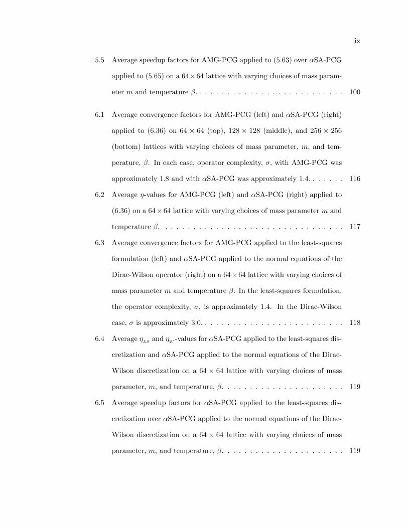
5.5 Average speedup factors for AMG-PCG applied to (5.63) over αSA-PCG

applied to (5.65) on a 64×64 lattice with varying choices of mass param-

eter m and temperature β. . . . . . . . . . . . . . . . . . . . . . . . . . . 100

6.1 Average convergence factors for AMG-PCG (left) and αSA-PCG (right)

applied to (6.36) on 64 × 64 (top), 128 × 128 (middle), and 256 × 256

(bottom) lattices with varying choices of mass parameter, m, and tem-

perature, β. In each case, operator complexity, σ, with AMG-PCG was

approximately 1.8 and with αSA-PCG was approximately 1.4. . . . . . . 116

6.2 Average η-values for AMG-PCG (left) and αSA-PCG (right) applied to

(6.36) on a 64× 64 lattice with varying choices of mass parameter m and

temperature β. . . . . . . . . . . . . . . . . . . . . . . . . . . . . . . . . 117

6.3 Average convergence factors for AMG-PCG applied to the least-squares

formulation (left) and αSA-PCG applied to the normal equations of the

Dirac-Wilson operator (right) on a 64×64 lattice with varying choices of

mass parameter m and temperature β. In the least-squares formulation,

the operator complexity, σ, is approximately 1.4. In the Dirac-Wilson

case, σ is approximately 3.0. . . . . . . . . . . . . . . . . . . . . . . . . . 118

6.4 Average ηLS and ηW -values for αSA-PCG applied to the least-squares dis-

cretization and αSA-PCG applied to the normal equations of the Dirac-

Wilson discretization on a 64 × 64 lattice with varying choices of mass

parameter, m, and temperature, β. . . . . . . . . . . . . . . . . . . . . . 119

6.5 Average speedup factors for αSA-PCG applied to the least-squares dis-

cretization over αSA-PCG applied to the normal equations of the Dirac-

Wilson discretization on a 64 × 64 lattice with varying choices of mass

parameter, m, and temperature, β. . . . . . . . . . . . . . . . . . . . . . 119

x

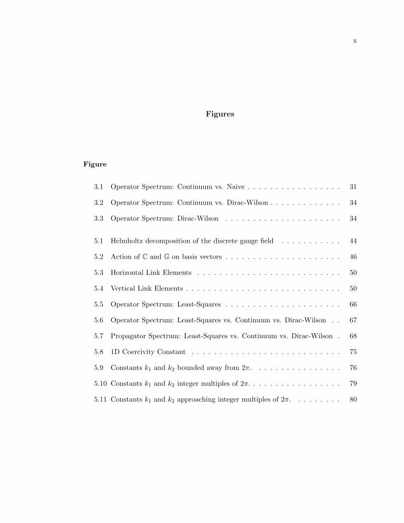
Figures

Figure

3.1 Operator Spectrum: Continuum vs. Naive . . . . . . . . . . . . . . . . . 31

3.2 Operator Spectrum: Continuum vs. Dirac-Wilson . . . . . . . . . . . . . 34

3.3 Operator Spectrum: Dirac-Wilson . . . . . . . . . . . . . . . . . . . . . 34

5.1 Helmholtz decomposition of the discrete gauge field . . . . . . . . . . . 44

5.2 Action of C and G on basis vectors . . . . . . . . . . . . . . . . . . . . . 46

5.3 Horizontal Link Elements . . . . . . . . . . . . . . . . . . . . . . . . . . 50

5.4 Vertical Link Elements . . . . . . . . . . . . . . . . . . . . . . . . . . . . 50

5.5 Operator Spectrum: Least-Squares . . . . . . . . . . . . . . . . . . . . . 66

5.6 Operator Spectrum: Least-Squares vs. Continuum vs. Dirac-Wilson . . 67

5.7 Propagator Spectrum: Least-Squares vs. Continuum vs. Dirac-Wilson . 68

5.8 1D Coercivity Constant . . . . . . . . . . . . . . . . . . . . . . . . . . . 75

5.9 Constants k1 and k2 bounded away from 2π. . . . . . . . . . . . . . . . 76

5.10 Constants k1 and k2 integer multiples of 2π. . . . . . . . . . . . . . . . . 79

5.11 Constants k1 and k2 approaching integer multiples of 2π. . . . . . . . . 80

Chapter 1

Introduction

The numerical solution of the Dirac equation is the main computational bottle-

neck in the numerical simulation of both quantum electrodynamics (QED) and quan-

tum chromodynamics (QCD), both of which are part of the Standard Model of particle

physics [30]. In general, the Dirac equation describes the interaction of spin-12 particles,

or fermions, and the particles that carry force between them, or bosons. QED describes

the electroweak interactions between electrons and their force carrying photons. QCD

describes the strong interaction between quarks and their force carrying gluons. The

dimension and complexity of the formulation of the Dirac equation depends on the spe-

cific theory that it describes [32]. Compared to QED, QCD is an extremely complex

theory. As such, it is common practice to develop new methods first for QED, and

then latter extend them to QCD. In this thesis, we focus on a simplified model of QED

known as the Schwinger model.

The primary purpose of any numerical simulation of QED (or QCD) is to verify

the validity of the theory by comparing numerical predictions to experiments. Val-

ues of physical observables, like particle mass and momenta, are computed via Monte

Carlo methods and compared to like quantities measured in particle accelerator experi-

ments [29]. The vast majority of computation time in such simulations is spent inverting

the discrete Dirac operator. As such, it is of utmost necessity to develop efficient nu-

merical solvers for the solution of such systems. In traditional discretizations of the

2

Dirac equation the resulting matrix operator is large, sparse, and highly structured, but

has random coefficients and is extremely ill-conditioned. The two main parameters of

interest are the temperature (β) of the background gauge (boson) field and the fermion

mass (m). For small values of β (< 10), the entries in the Dirac matrix become highly

disordered. Moreover, as the fermion mass approaches its true physical value, perfor-

mance of the community standard Krylov solvers degrades - a phenomenon known as

critical slowing down [14]. As a result, the development of sophisticated preconditioners

for the solution process has been a priority in the physics community for some time.

The use of multilevel methods as preconditioners for solution of the Dirac equation were

first used in the 1990’s [22]. Though greatly improving solver performance, they did

not successfully eliminate critical slowing down. Recently, adaptive multilevel precon-

ditioners such as adaptive smoothed aggregation multigrid (αSA) have proved capable

of eliminating critical slowing down [13], [14].

In addition to developing fast solvers for traditional discretizations of the Dirac

operator, it is also necessary to consider alternate discretizations of the governing equa-

tions that, while capturing the physical properties of the continuum system, also lend

themselves to efficient solution by iterative methods. The vast majority of popular

discretizations utilize finite difference techniques. Due to the first-order nature of the

operator, the naive application of finite difference techniques results in a problem that

the physics community refers to as species doubling [29]. In the applied mathematics

community, this phenomenon is known as red-black instability. As such, modifications

of simple finite difference discretizations are necessary to avoid this issue. In the popular

Dirac-Wilson discretization the problem of species doubling is remedied by adding artifi-

cial diffusion to the main diagonal of the operator [52]. In [45], a nonlocal approximation

to the continuum normal equations is formulated using finite differences. Recently, new

methods have been have been developed, based on finite-differences, that retain many

important physical properties. However, these methods require formulating the prob-

3

lem in five dimensions, greatly increasing the computational cost needed to simulate

the theory [35], [38], [48]. The primary purpose of this thesis is to introduce consistent

discretization of the simplified Schwinger model using least-squares finite elements.

Finite element discretizations have been largely overlooked in lattice gauge the-

ory. Attempts were made in the 1990’s to employ finite element methods but were

quickly abandoned, primarily because typical Galerkin-like formulations fail to avoid

the problem of species doubling. In [31], the continuum equations are expanded in an

infinite set of Bloch wave functions and an approximation is obtained by restriction to

the lowest mode wave functions, which are very similar finite element basis functions.

The primary focus of this dissertation is the development of an alternate discretization

of the Dirac equation using least-squares finite elements. This formulation leads to a

discrete system that is consistent with the physical properties of the continuum govern-

ing equations, avoids the problem of species doubling, and is amenable to solution via

adaptive multilevel methods. It is the first formulation to date that accomplishes all of

these tasks without extending the model to a costly fifth dimension.

The layout of the thesis is as follows. In Chapter 2, we introduce the general

continuum Dirac operator. We discuss the formulations of the model for QED, QCD,

and the simplified Schwinger model. We also discuss an alternative formulation of

the Schwinger model that will prove useful in our analysis of discretization methods.

Finally, we discuss various physical properties that the continuum operator satisfies,

including gauge covariance and chiral symmetry. In Chapter 3, we discuss various

discrete approximations to the continuum model. We introduce the method of covariant

finite differences and traditional discretizations that result from their use, including the

Naive discretization and Wilson’s discretization. We formulate discrete analogues of

gauge covariance and chiral symmetry, as well as discuss the concept of species doubling.

Finally, we discuss the numerical advantages and disadvantages of building simulations

around these discretizations. Chapters 2 and 3 are intended to serve as a stand-alone

4

introduction to discretizations of the Dirac operator for the applied mathematician with

little to no background in lattice gauge theory.

Chapter 4 introduces the general least-squares finite element discretization that

is the primary method used in this thesis. We discuss the method applied to a general

first-order system of PDEs. In Chapter 5, we apply the least-squares finite element

methodology to the Schwinger model of QED. A gauge covariant solution process is

obtained directly from the standard formulation of the governing equations by applying

a method known as gauge fixing. It is then demonstrated that the resulting linear system

satisfies chiral symmetry and does not suffer from species doubling. The spectrum of

the resulting discrete operator is then compared to that of the continuum operator.

Finally, it is demonstrated that the least-squares functional satisfies an H1-ellipticity

property, and implications of this are discussed. In the remainder of the chapter, the

application of an algebraic multigrid as a preconditioner for the solution process is

investigated. It is demonstrated that the resulting linear system of equations can be

solved efficiently using such a multilevel method. Finally, we compare the performance

of two algebraic multigrid methods applied to the discrete least-squares system and

a traditional discretization based on covariant finite differences. It is shown that the

former can be solved roughly twice as fast as the latter.

In Chapter 6, the least-squares methodology is applied to an alternate formula-

tion of the governing equations that employs a transformation based on a Helmholtz

decomposition of the gauge field. This effectively removes the gauge field from the differ-

ential operators and yields a linear system similar to a diffusion equation with variable

coefficients. It is shown that the resulting linear system satisfies gauge covariance and

chiral symmetry, and does not suffer from species doubling. Next, the H1-ellipticity of

the least-squares functional is established. Finally, the use of two algebraic multigrid

methods are investigated as preconditioners in the solution process. These methods are

shown to be very effective at solving the resulting system of equations.

5

Finally, in Chapter 7, we make concluding remarks and discuss future directions

of the project.

Chapter 2

The Continuum Model

In this chapter, detailed background of the Dirac operator is presented. First, the

continuum Dirac operator is introduced together with several properties that it must

satisfy, including gauge covariance and chiral symmetry. Next, the discrete Dirac op-

erator and the discrete analogues of the previously mentioned physical properties are

discussed. To motivate this, two traditional discretizations of the Dirac operator are

considered: the so-called naive discretization and Wilson’s discretization. The proper-

ties of gauge covariance and chiral symmetry are discussed in terms of the two resulting

discrete operators and, in the process, the curious phenomenon of species doubling is

introduced.

2.1 Continuum Dirac Operator

The Dirac equation is the relativistic analogue of the Schrodinger equation [32].

It describes the interaction between spin-12 particles, called fermions, and the particles

that carry force between them, aptly termed force carriers. Depending on the specific

gauge theory, the operator can take on several forms, the most general of which is given

by

Dψ =d∑

µ=1

γµ ⊗ (∂µI − iAµ)ψ +mψ. (2.1)

7

Here, d is the problem dimension, γµ is a set of matrix coefficients, ∂µ is the usual

partial derivative in the xµ direction, m is the particle mass, and Aµ (x) is a matrix

operator describing the gauge field. In quantum electrodynamics (QED) and quantum

chromodynamics (QCD) we wish to describe particles of different spins and colors. The

dimensions of matrices γµ and Aµ depend on the number of spins in the theory, ns, and

the number of colors in the theory, nc. Specifically, each γµ is ns×ns and Aµ is nc×nc.

Operator D acts on ψ : Rd 7→ Cns ⊗Cnc , a tensor field (multicomponent wavefunction)

describing the particle. It is common to refer to the inverse Dirac operator, D−1, as the

fermion propagator. We introduce the shorthand notation ∇µ = ∂µI − iAµ for the µth

covariant derivative. Occasionally, we wish to explicitly indicate that operator D, and

its propagator, depend on gauge field A. Thus, we denote the Dirac operator by D (A)

and its propagator by D−1(A).

Quantum electrodynamics, with which this thesis is most concerned, is the study

of the interaction of electrically charged fermions, electrons, and their force carriers,

photons. In the full physical model of QED, particles can have one of four different

spins, so ns = 4. The term spin here is slightly ambiguous. In addition to a particle

having a specific angular momentum, either spin-up or spin-down, it also has a specific

energy, either positive or negative. The energies here distinguish between particles and

anti-particles. The anti-particle of the electron is the positron. The two possible spins

and energies then lead to four possible types of particles: spin-up electrons, spin-down

electrons, spin-up positrons, and spin-down positrons. The concept of color is specific

to QCD, so, in the case of QED, nc = 1.

The set of matrix coefficients, γµ, do not have a definite form. They must simply

form a basis for the set of ns × ns unitary, anti-commuting matrices. A Traditional

choice are the so-called Dirac matrices:

8

γ1 =

0 0 0 1

0 0 1 0

0 1 0 0

1 0 0 0

, γ2 =

0 0 0 −i

0 0 i 0

0 −i 0 0

i 0 0 0

,

γ3 =

0 0 1 0

0 0 0 −1

1 0 0 0

0 −1 0 0

, γ4 =

0 0 −i 0

0 0 0 −i

i 0 0 0

0 i 0 0

.

The full physical theory has four dimensions (one temporal and three spatial). With

the above given choice for γµ, the Dirac operator becomes

mI 0 ∇3 − i∇4 ∇1 − i∇2

0 mI ∇1 + i∇2 −∇3 − i∇4

∇3 + i∇4 ∇1 − i∇2 mI 0

∇1 + i∇2 −∇3 + i∇4 0 mI

ψ1

ψ2

ψ3

ψ4

=

f1

f2

f3

f4

, (2.2)

where ψs and fs, s = 1, . . . , 4, correspond to the sth spin component of ψ and f ,

respectively. With nc = 1, ∂µI and Aµ become scalar operators. The gauge field, A,

has four components, Aµ (x) ∈ R, each representing the photons in one of the four

directions.

Quantum chromodynamics describes the interaction of color charged particles.

The fermion in this case is a quark. The carriers of the color-force are the gluons. Color

charged particles can be red, blue, or green. Like QED, particles come in four different

spins (spin-up quark, spin-down quark, spin-up anti-quark, and spin-down anti-quark).

However, each of these spin components can be a specific color as well, leading to twelve

distinct types of particles. (Note that color here does not refer to the actual visible

9

color of the particle: it is simply an arbitrary construct of the theory.) Again, like in

QED, the theory is typically represented in four dimensions. The formulation of the

Dirac equation in quantum chromodynamics is structurally similar to (2.2), but the

dimensions of ∇µ must be altered to account for the three colors of particles. Because

the gauge field must describe the interaction of particles of three different colors, we

have Aµ ∈ su(3), the space of 3 × 3, traceless, Hermitian matrices. The µth covariant

derivative operator acting on the sth spin component of ψ appears as

∇µψs =

∂xµ 0 0

0 ∂xµ 0

0 0 ∂xµ

− iAµ

ψs,r

ψs,g

ψs,b

, (2.3)

where r, g, and b indicate the color of the particle. The QCD form of the Dirac

equation appears exactly as in (2.2), but instead of ψs being a scalar quantity, it is a

three-component wavefunction, with each component describing a particle of a certain

color.

Describing ψ as a wavefunction necessarily indicates a relationship between ψ and

a probability amplitude. That is, suppose that p represents, for instance, the state of a

quark being spin-up, having positive energy, and being green. Then

∫V|ψp|2dV, (2.4)

is the probability that the particle in question is spin-up, has positive energy, is green,

and can be found in the spatial region V [32].

Finally, it is useful to make some observations about the spectral properties of D.

Since we are discretizing D, it is desirable that the spectrum of the resulting discrete

operator has a spectrum at least somewhat similar to that of the continuum operator.

10

Note that, in both the QED and QCD cases, the covariant derivative operators are

anti-Hermitian. That is,

∇∗µ = −∇µ, (2.5)

where L∗ represents the formal adjoint of differential operator L. Then, it is easy to see

that (2.2) can be written as

D =

mI B

−B∗ mI

, (2.6)

where B : Rd 7→ Cns/2 ⊗ Cnc . Further, D can be decomposed into a sum of Hermitian

and anti-Hermitian matrices, according to

D =

mI 0

0 mI

+

0 B

−B∗ 0

. (2.7)

It then follows that the eigenvalues of D lie on a vertical line in the complex plain,

intersecting the real axis at m. That is,

Σ (D) = m+ is, (2.8)

where m, s ∈ R. Then, the eigenvalues of the fermion propagator, D−1, are given by

Σ(D−1

)=

1

m+ is, (2.9)

where, again, s ∈ R. That is, the eigenvalues of the propagator lie on a circle in the

complex plane with radius 12m , and centered on the real axis at 1

2m .

11

2.2 The Schwinger Model

The operator D, in both QED and QCD, is complicated, to say the least. In four

dimensions, with four spins, and three colors, the size of any discrete representation

can get intractably large. As such, it is common to work with a simplified systems

rather than the full physical models [14]. The so-called Schwinger Model is a two-spin

model of QED in two spatial dimensions. Like the full physical model of QED it can

be considered a model of the interaction between electrons and photons. Rather than

four different types of particles though, it models only two, which we refer to as left-

and right-handed. Here, handedness, or helicity, is a characterization of a particle’s

angular momentum relative to its direction of motion. For massive particles, left- and

right-handed are analogous to spin-up and spin-down particles, respectively. In two

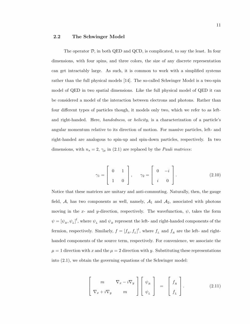
dimensions, with ns = 2, γµ in (2.1) are replaced by the Pauli matrices:

γ1 =

0 1

1 0

, γ2 =

0 −i

i 0

. (2.10)

Notice that these matrices are unitary and anti-commuting. Naturally, then, the gauge

field, A, has two components as well, namely, A1 and A2, associated with photons

moving in the x- and y-direction, respectively. The wavefunction, ψ, takes the form

ψ = [ψR , ψL ]t, where ψL and ψR represent the left- and right-handed components of the

fermion, respectively. Similarly, f = [fR , fL ]t, where fL and fR are the left- and right-

handed components of the source term, respectively. For convenience, we associate the

µ = 1 direction with x and the µ = 2 direction with y. Substituting these representations

into (2.1), we obtain the governing equations of the Schwinger model:

m ∇x − i∇y

∇x + i∇y m

ψR

ψL

=

fR

fL

. (2.11)

12

Naturally, the physical objects that are modeled by equations such as these can

act on extremely large spatial domains. It is natural then to restrict our attention to

a small physical domain and require that the wavefunction, ψ, and the gauge field, A,

be periodic on that domain. Let that domain be R = [0, 1] × [0, 1]. Then, let VR be

some space of real-valued, periodic functions on R, and VC be some space of complex-

valued, periodic functions on R. The specific characteristics of spaces VR and VC are

discussed in a later chapter. Let ψ (x, y) = [ψR (x, y) , ψL (x, y)]t ∈ V2C be the fermion

field with right- and left-handed components ψR and ψL , respectively. Assume that

A (x, y) = [A1 (x, y) ,A2 (x, y)]t ∈ V2R . With periodic boundary conditions on ψ, the 2D

Schwinger model becomes

mI ∇x − i∇y

∇x + i∇y mI

ψR

ψL

=

fR

fL

in R, (2.12)

ψ(0, y) = ψ(1, y) ∀y ∈ (0, 1),

ψ(x, 0) = ψ(x, 1) ∀x ∈ (0, 1),

Note that the Schwinger model is a specific version of the Dirac equation. As

such, in the remainder of this thesis, the two terms are used interchangeably. If, at

some time, the full physical version of the Dirac operator is discussed, it will be made

clear from context that we are speaking of something other than the Schwinger model.

2.2.1 Gauge Covariance

In any gauge theory, like QED or QCD, several physical symmetries of the system

must be captured by the Dirac operator. This section is concerned with the manner

in which the Dirac operator transforms under both local and global modifications of

the fermion field. The first such symmetry discussed is a local gauge symmetry. In

this case, the fermion propagators, D−1, must transform covariantly under local gauge

13

transformations [29]. A local gauge transformations, denoted by Ω (x, y), is a member of

the gauge group of the theory. In QED, Ω (x, y) ∈ U(1), the set of complex scalars with

unit magnitude. In QCD, Ω (x, y) ∈ SU(3), the set of complex, unitary, 3× 3 matrices

with determinant one. The transformation is local because it depends on x and y.

Definition 2.2.1. Suppose a local gauge transformation, Ω (x, y), is applied to each

component of the fermion field ξ. Then, a modified propagator, D−1, must exist such

that

D−1 [Ω (x, y) Ins ] ξ = [Ω (x, y) Ins ] D−1ξ, (2.13)

where Ins is the ns × ns identity operator, and transformation Ω (x, y) is a member of

the gauge group.

To find the appropriate form of D, we consider the form of the Schwinger model

appearing in (2.12). In the Schwinger case, the condition for the gauge covariance of

D−1 can be written as

D−1

Ω (x, y) 0

0 Ω (x, y)

ξ =

Ω (x, y) 0

0 Ω (x, y)

D−1ξ. (2.14)

Let Ω (x, y) = eiω(x,y) for some real, periodic function ω. Suppose further that D is

constructed using the gauge field, A = [A1,A2]t. We make the ansatz that the modified

Dirac operator, D, has the same form as the original operator, but is built using a

modified gauge field, A =[A1, A2

]t. For simplicity, write D as

D = γ1 ⊗ ∇x + γ2 ⊗ ∇y +mI,

where ∇x = ∂x − iA1 and ∇y = ∂y − iA2. Equating the right-hand side of (2.14) with

some fermion field, ζ, yields

14

Ω (x, y)[γ1 ⊗ ∇x + γ2 ⊗ ∇y +mI

]−1ξ = ζ.

Then,

ξ =[γ1 ⊗ ∇x + γ2 ⊗ ∇y +mI

]Ω∗ (x, y) ζ

= γ1 ⊗ ∇x(e−iωζ

)+ γ2 ⊗ ∇y

(e−iωζ

)+mI

(e−iωζ

)= γ1 ⊗

(∂x − iA1

) (e−iωζ

)+ γ2 ⊗

(∂y − iA2

) (e−iωζ

)+mI

(e−iω

)ζ

= Ω∗ (x, y)[γ1 ⊗

(∂x − iA1 + ωx

)+ γ2 ⊗

(∂y − iA2 + ωy

)+mI

]ζ,

where ωx = ∂xω and ωy = ∂yω. Thus,

[γ1 ⊗

(∂x − iA1 + ωx

)+ γ2 ⊗

(∂y − iA2 + ωy

)+mI

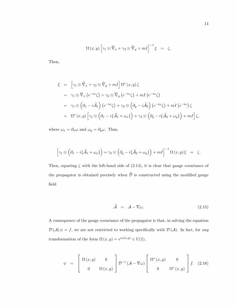
]−1Ω (x, y) ξ = ζ.

Then, equating ζ with the left-hand side of (2.14), it is clear that gauge covariance of

the propagator is obtained precisely when D is constructed using the modified gauge

field

A = A−∇ω. (2.15)

A consequence of the gauge covariance of the propagator is that, in solving the equation

D (A)ψ = f , we are not restricted to working specifically with D (A). In fact, for any

transformation of the form Ω (x, y) = eiω(x,y) ∈ U(1),

ψ =

Ω (x, y) 0

0 Ω (x, y)

D−1 (A−∇ω)

Ω∗ (x, y) 0

0 Ω∗ (x, y)

f. (2.16)

15

Then, it is possible to solve the original problem for ψ by first applying the inverse

transform to the source term, f , applying the transformed propagator, D−1 (A−∇ω),

and then applying the transform to the result.

An interesting physical implication for the property of gauge covariance is more

clearly explained in the context of QCD. The application of a gauge transformation to

a fermion field, ψ, can be viewed as a change in the color reference frame. A trivial

example would be if the roles of blue and red particles were interchanged in the model.

Since the gauge transformation depends on the location in the domain, it is also possible

to, for instance, interchange the role of blue and red particles in the first quadrant of

the domain, interchange the role of red and green particles in the second quadrant, and

leave the remainder of the domain unaffected. Let C denote the original color reference

frame, and C denote the modified reference frame described above. Then, in accordance

with (2.16), given the problem D (A)ψ = f in reference frame C, we can solve for ψ

by transforming the source data into reference frame C, inverting the analogous Dirac

operator there and, then, transforming the result back to reference frame C.

This property illuminates a fundamental relationship between gauge fields, A and

A, which differ only by the gradient of a periodic function. Essentially, any computation

that can be done with A could, in fact, be done with A instead. Such pairs of gauge

fields are said to be in the same equivalence class.

Definition 2.2.2. Gauge fields A and A are said to be in the same equivalence class if

there exists some differentiable periodic function, ω (x, y), such that

A = A−∇ω.

Gauge covariance is perhaps the most crucial property in a theory such as QED.

The Monte Carlo simulation at the heart of these simulations is, in fact, an approxi-

16

mation of an infinite-dimensional Feynman path integral [27]. In such an integral, it

is necessary to integrate over all possible gauge fields. With the property of gauge

covariance of the propagator intact, the problem is reduced to integrating over all pos-

sible gauge field equivalence classes instead. This clearly reduces the dimensionality the

continuum problem, as well as any discrete approximation of the process.

2.2.2 Chiral Symmetry

The second physical property that should be conserved is chiral symmetry. In

the broadest sense, chiral symmetry is the global symmetry property that indepen-

dent transformations of the right- and left-handed fields do not change the physics of

the model in the massless case [29]. This property is manifested mathematically by

the property that, when m = 0, the inner product 〈ξ, γ1Dξ〉 remains invariant under

transformations of the form ξ 7→ Λξ, where 〈· , ·〉 is the usual L2 inner product, and

Λ =

eiλR 0

0 eiλL

, (2.17)

for λR , λL ∈ R.

Definition 2.2.3. Given λR , λL ∈ R, and transformation Λ defined by

Λ =

eiλR 0

0 eiλL

, (2.18)

operator D satisfies a chiral symmetry if, for m = 0,

〈Λξ, γ1DΛξ〉 = 〈ξ, γ1Dξ〉 . (2.19)

where 〈 · , · 〉 is the usual L2 inner product.

17

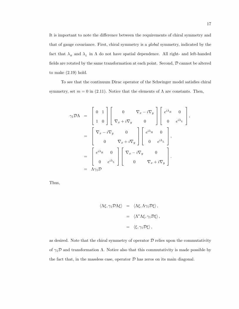
It is important to note the difference between the requirements of chiral symmetry and

that of gauge covariance. First, chiral symmetry is a global symmetry, indicated by the

fact that λR and λL in Λ do not have spatial dependence. All right- and left-handed

fields are rotated by the same transformation at each point. Second, D cannot be altered

to make (2.19) hold.

To see that the continuum Dirac operator of the Schwinger model satisfies chiral

symmetry, set m = 0 in (2.11). Notice that the elements of Λ are constants. Then,

γ1DΛ =

0 1

1 0

0 ∇x − i∇y

∇x + i∇y 0

eiλR 0

0 eiλL

,

=

∇x − i∇y 0

0 ∇x + i∇y

eiλR 0

0 eiλL

,

=

eiλR 0

0 eiλL

∇x − i∇y 0

0 ∇x + i∇y

.= Λγ1D

Thus,

〈Λξ, γ1DΛξ〉 = 〈Λξ,Λγ1Dξ〉 ,

= 〈Λ∗Λξ, γ1Dξ〉 ,

= 〈ξ, γ1Dξ〉 ,

as desired. Note that the chiral symmetry of operator D relies upon the commutativity

of γ1D and transformation Λ. Notice also that this commutativity is made possible by

the fact that, in the massless case, operator D has zeros on its main diagonal.

18

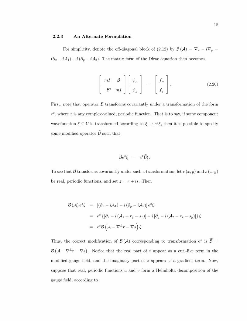
2.2.3 An Alternate Formulation

For simplicity, denote the off-diagonal block of (2.12) by B (A) = ∇x − i∇y =

(∂x − iA1)− i (∂y − iA2). The matrix form of the Dirac equation then becomes

mI B

−B∗ mI

ψR

ψL

=

fR

fL

. (2.20)

First, note that operator B transforms covariantly under a transformation of the form

ez, where z is any complex-valued, periodic function. That is to say, if some component

wavefunction ξ ∈ V is transformed according to ξ 7→ ezξ, then it is possible to specify

some modified operator B such that

Bezξ = ezBξ.

To see that B transforms covariantly under such a transformation, let r (x, y) and s (x, y)

be real, periodic functions, and set z = r + is. Then

B (A) ezξ = [(∂x − iA1)− i (∂y − iA2)] ezξ

= ez [∂x − i (A1 + ry − sx)]− i [∂y − i (A2 − rx − sy)] ξ

= ezB(A−∇⊥r −∇s

)ξ.

Thus, the correct modification of B (A) corresponding to transformation ez is B =

B(A−∇⊥r −∇s

). Notice that the real part of z appear as a curl-like term in the

modified gauge field, and the imaginary part of z appears as a gradient term. Now,

suppose that real, periodic functions u and v form a Helmholtz decomposition of the

gauge field, according to

19

A =

A1

A2

= ∇⊥u+∇v +

k1

k2

, (2.21)

where k1 and k2 are constants. Setting z = u+ iv yields

B (A) ezξ = ezBkξ, (2.22)

where Bk := (∂x − ik1) − i (∂y − ik2). In addition, it is easy to verify that the adjoint

operator, B∗, transforms covariantly under a similar transformation. Specifically,

B∗ (A) e−zξ = e−zB∗kξ. (2.23)

From (2.22) and (2.23), it is easy to see that B (A) and its adjoint can be written as

B (A) = ezBke−z, (2.24)

B∗ (A) = e−zB∗kez, (2.25)

where z = u + iv. This representation gives insight into the nullspace of B. First,

consider the transformed operator Bk, with the non-constant portion of the gauge field

removed. Let φ = ei(k1x+k2y). Then

Bkφ = [(∂x − ik1)− i (∂y − ik2)] ei(k1x+k2y),

= [(ik1 − ik1)− i (ik2 − ik2)] ei(k1x+k2y),

= 0.

But, recall that operator Bk acts on complex-valued periodic functions, and that

20

ei(k1x+k2y) = [cos (k1x) + i sin (k1x)] [cos (k2y) + i sin (k2y)] .

Then, φ = ei(k1x+k2y) is periodic onR only if k1 = 2πl1 and k2 = 2πl2 for some l1, l2 ∈ Z.

Thus, it is easy to see from (2.24) that operator B (A) is singular, with nullspace vector

φ = ez+i(k1x+k2y), only if k1 and k2 are integer multiples of 2π. Similarly, from (2.25)

it is clear that, under these conditions on k, B∗ (A) is singular with nullspace vector

φ = e−z+i(k1x+k2y) [36].

Next, notice that (2.20) can be reformulated as

mI ezBke−z

−e−zB∗kez mI

ψR

ψL

=

fR

fL

. (2.26)

Then, if the constant portions of the gauge field are integer multiples of 2π, D has two

eigenvectors, φ+ and φ−, associated with purely real eigenvalue m, where

φ+ =

e−z+i(k1x+k2y)

ez+i(k1x+k2y)

, (2.27)

φ− =

−e−z+i(k1x+k2y)

−ez+i(k1x+k2y)

. (2.28)

We refer to a gauge field with these properties as an exceptional configuration.

Definition 2.2.4. Let gauge field A have the Helmholtz decomposition given in (2.21).

Gauge field A is an exceptional configuration if constants k1 and k2 are integer multiples

of 2π.

Furthermore, if A is an exceptional configuration, the massless Dirac operator, D0, is

singular, with nullspace vectors in the span of φ+ and φ−. This clearly has implications

for any discretization of D, because any matrix approximation, D, that shares this

21

spectral characteristic will become increasingly ill-conditioned as m → 0. However, if

either k1 or k2 is not an integer multiple of 2π, B will not be singular and, by extension,

D will not have any purely real eigenvalues.

Chapter 3

The Discrete Model

In numerical simulations of QED, many solutions of the discrete Dirac equation

must be computed for varying gauge fields and source vectors. Solutions of systems

of this type are needed both for computing observables and for generating gauge fields

with the correct probabilistic characteristics [13]. In traditional lattice formulations,

the continuum domain, R, is replaced by an N × N regular, periodic lattice. The

continuum wavefunction, ψ, and source, f , are replaced by periodic discrete analogues,

ψ and f , with values specified only at the lattice sites. The continuum gauge field, A,

is represented by the periodic discrete field A = [A1, A2]t, with information specified on

each of the lattice links. The components of the gauge field, A1 and A2, represent values

on the horizontal and vertical lattice links, respectively. A discrete solution process of

the 2D Schwinger model then takes the source, f , specified at the lattice sites and

gauge field, A, specified at the lattice links, and returns the discrete fermion field, ψ,

with values again specified at the lattice sites. The discrete solution can be written as

ψ = [D (A)]−1 f,

where D is some discrete approximation of the continuum Dirac operator.

For completeness, let NC be the space of discrete complex-valued vectors with

values associated with the sites on the lattice. Let NR ⊂ NC be the space of discrete

23

real-valued vectors, with values associated with the lattice sites. Then, the discrete

fermion field is given by ψ = [ψR, ψ

L]t ∈ N 2

C , which specifies complex values of both the

right- and left-handed components of the fermion field at each lattice site. Similarly,

f = [fR, f

L]t ∈ N 2

C . Let E be the space of discrete real-valued vectors with values

associated with the lattice links. Then A = [A1, A2]t ∈ E .

3.1 The Naive Discretization

Traditional discretizations of the Dirac equation are based on covariant finite

differences. As the name suggests, this method produces a discrete operator by applying

a finite difference-like approximation of the covariant derivative, ∇µ. In this chapter, we

consider two such discretizations: the Naive discretization and the Wilson discretization

[29]. The former produces the following discrete operator in the Schwinger case:

DN =

mI ∇hx − i∇hy

∇hx + i∇hy mI

, (3.1)

where ∇hx and ∇hy , acting on the right-hand component of ψ, have the following centered

difference formulas:

∇hxψRj,k

=1

2h

(eiθj+1/2,kψ

Rj+1,k− e−iθj−1/2,kψ

Rj−1,k

), (3.2)

∇hyψRj,k

=1

2h

(eiθj,k+1/2ψ

Rj,k+1− e−iθj,k−1/2ψ

Rj,k−1

). (3.3)

The values of θ, called phase factors, are located at the midpoint of lattice links and

relate to the continuum gauge field according to

θj+1/2,k =

∫ xj+1

xj

A1 (x, yk) dx, (3.4)

θj,k+1/2 =

∫ yk+1

yk

A2 (xj , y) dy. (3.5)

24

Note that because A is a real-valued function, the phase factors are real-valued as well.

As a result, the coefficients in the covariant finite differences are members of the gauge

group U(1). Denote the collection of phase factors associated with both the horizontal

and vertical lattice links by θ. Notice then that θ ∈ E . It can be shown that the

covariant finite differences converge to the associated continuum covariant derivatives

as the lattice spacing goes to zero. Matrix DN can be written in the simplified form

DN =

mI BN

−B∗N mI

, (3.6)

where B∗N is the conjugate transpose of matrix BN , with stencil

BN =1

2h

−ieiθj,k+1/2

−e−iθj−1/2,k 0 eiθj+1/2,k

ie−iθj,k−1/2

. (3.7)

Notice that (3.6), like its continuum analogue (2.6), can be decomposed into Hermitian

and anti-Hermitian parts:

D =

mI 0

0 mI

+

0 BN

−B∗N 0

. (3.8)

Thus, as in the continuum case, the eigenvalues of DN lie on a vertical line in the

complex plain intersecting the real axis at m. That is,

Σ (DN ) = m+ isj , j = 1, . . . , 2n2, (3.9)

where sj ∈ R. The fact that the eigenvalues of the discrete operator lie on the same

vertical line in the complex plane as the eigenvalues of the continuum operator is en-

25

couraging. Unfortunately, we will see later that the actual values of the discrete and

continuum eigenvalues do not agree well at all.

3.1.1 Gauge Covariance

As in the continuum case, matrix operator DN must satisfy discrete analogues of

gauge covariance and chiral symmetry. Recall that, in the continuum, a gauge transfor-

mation, Ω, is defined by

Ω (x, y) = eiω(x,y),

where ω (x, y) is a periodic, real-valued function. Let ω be the vector whose entries are

the values of ω (x, y) evaluated at each lattice site. That is,

ωj,k = ω (xj , yk) .

Then, define a discrete gauge transformation, Ωω, by the n2×n2 diagonal matrix, whose

entries are given by

[Ωω

]l,l

= eiωj,k , (3.10)

and the map between l and (j, k) is defined by the usual lexicographic ordering of

the unknowns. Note that Ωω is a unitary matrix and that each of its entries is itself a

member of the gauge group U(1). Also, note that the adjoint, Ω∗ω, is simply the diagonal

matrix whose entries are the complex conjugates of the diagonal entries of Ωω. Finally,

define unitary matrices Tω and T∗ω according to

Tω =

Ωω 0

0 Ωω

T∗ω =

Ω∗ω 0

0 Ω∗ω

.

26

Recalling Definition 2.2.1, we make the following definition of gauge covariance

of the discrete solution process:

Definition 3.1.1. Suppose a discrete local gauge transformation, Ωω, is applied to each

component of the discrete fermion field, ξ. A discrete solution process is gauge covariant

if a modified discrete propagator, D−1, exists such that

D−1Tω ξ = Tω D−1ξ. (3.11)

A little algebra shows that (3.11) is equivalent to

Tω Dζ = DTω ζ, (3.12)

for ζ = D−1ξ. In general, to determine the form of D, it is only necessary to consider

(3.12) for a single arbitrary row of the equation. We wish to show that the Naive Dirac

operator, DN , satisfies this definition of gauge covariance. Without loss of generality,

consider only the j, kth component of ζR

. Again, we make the ansatz that DN and DN

only differ in their gauge data, θ and θ, respectively. For simplicity of notation, we

require that the stencils for ζRj,k

satisfy

1

2h

−iei(θj,k+1/2+ωj,k+1)

−e−i(θj−1/2,k−ωj−1,k) 0 ei(θj+1/2,k+ωj+1,k)

ie−i(θj,k+1/2−ωj,k−1)

=1

2h

−iei(θj,k+1/2+ωj,k)

−e−i(θj−1/2,k−ωj,k) 0 ei(θj+1/2,k+ωj,k)

ie−i(θj,k+1/2−ωj,k)

. (3.13)

Clearly then, (3.12) is satisfied when

27

θj+1/2,k = θj+1/2,k −(ωj+1,k − ωj,k

),

θj−1/2,k = θj−1/2,k −(ωj,k − ωj−1,k

),

θj,k+1/2 = θj,k+1/2 −(ωj,k+1 − ωj,k

),

θj,k−1/2 = θj,k−1/2 −(ωj,k − ωj,k−1

),

which, in turn, implies that DN satisfies Definition 3.1.1. Recall that, in the contin-

uum case, the correct modification of D required subtracting ∇ω from the given gauge

field. This is precisely the modification that was necessary in the discrete case. In this

instance, a constant multiple of a discrete gradient of ω is subtracted from each of the

original phase factors.

3.1.2 Chiral Symmetry

Similarly, we require a discrete analogue of Definition 2.2.3 for chiral symmetry.

In the discrete case, chiral symmetry requires that, in the massless case, the physics

remained unchanged under independent transformation of the left- and right-handed

components of the discrete fermion field.

Definition 3.1.2. Suppose λR , λL ∈ R, and a transformation Λ is defined by

Λ =

eiλR I 0

0 eiλL I

, (3.14)

where I is the n2 × n2 identity matrix. Operator D satisfies a chiral symmetry if, for

m = 0,

⟨Λξ,Γ1DΛξ

⟩=

⟨ξ,Γ1Dξ

⟩, (3.15)

28

where

Γ1 =

0 I

I 0

, (3.16)

and 〈 · , · 〉 is the usual discrete l2 inner product.

In the following lemma, we verify that the Naive discrete Dirac operator, DN , satisfies

chiral symmetry.

Lemma 3.1.3. The Naive Dirac operator, DN , satisfies chiral symmetry.

Proof. Let λR , λL ∈ R and define DN , Λ, and Γ1 according to (3.6), (3.14), and (3.16),

respectively. Setting m = 0, DN becomes

DN =

0 BN

−B∗N 0

. (3.17)

Then,

⟨Λξ,Γ1DNΛξ

⟩=

⟨Λ∗D∗NΓ1Λξ, ξ

⟩.

Simplifying the long matrix product gives

Λ∗D∗NΓ1Λ =

e−iλR I 0

0 e−iλL I

BN 0

0 −B∗N

eiλR I 0

0 eiλL I

=

e−iλR I 0

0 e−iλL I

eiλR I 0

0 eiλL I

BN 0

0 −B∗N

=

BN 0

0 −B∗N

= D∗NΓ1.

29

Notice that commutation performed in the second line above is only valid because λR

and λL are constant. Furthermore, if a mass term were present, the above commutation

would not be valid. Finally,

⟨Λξ,Γ1DNΛξ

⟩=

⟨D∗NΓ1ξ, ξ

⟩=

⟨ξ,Γ1DNξ

⟩,

as desired.

3.1.3 Species Doubling

Thus far, the Naive Dirac operator, DN , has shown a great deal of promise. The

discretization is simple, it agrees spectrally with the continuum operator, and it satisfies

discrete versions of gauge covariance and chiral symmetry. There is, however, a major

problem with the discretization, which we illustrate here using a 1D version of the

Schwinger model. In 1D, the Naive Dirac operator is given by

DN = γ1 ⊗∇hx +mI, (3.18)

where ∇hx has the stencil previously given in (3.3). In the gauge-free case (that is,

A = 0), operator ∇hx, acting on the right-handed component of ψ, becomes

∇hxψRj,k

=1

2h

(ψRj+1,k

− ψRj−1,k

), (3.19)

where h is the lattice spacing. In the 1D free case,

DN =

mI Bx

Bx mI

, (3.20)

30

where Bx is the periodic Toeplitz matrix with stencil 1h [−1/2 0 1/2]. For simplicity,

assume that the 1D lattice has N cells and, thus, N + 1 periodic lattice sites, and that

N is even. Then, the eigenvalues of Bx are given by

νk =i

hsin

(2πk

N

), (3.21)

for k = − (N/2− 1) , . . . , N/2. Note that νk and ν−k, for k = 1, . . . , N/2, are complex

conjugate pairs. It is clear from the form of DN that the eigenvalues of the discrete

propagator, D−1N , are given by

κk =h

mh+ isin (2πk/N), (3.22)

with corresponding eigenvectors

vk =

[1, 1, . . . , 1, 1]t k = 0,

[. . . , cos (2πk`/N)± sin (2πk`/N) , . . .]t k = ±1, . . . , N/2− 1,

[1,−1, . . . , 1,−1]t k = N/2,

(3.23)

where l = 1, . . . , n. Notice the symmetry of κk. For every low frequency eigenvector,

a corresponding high frequency eigenvector shares the same eigenvalue. The physics

community is especially concerned with the correspondence between the eigenvalues of

the k = 0 and k = N/2 modes. In the Naive discretization, the eigenvalues of the

propagator, D−1N , associated with these two modes both approach∞ as m→ 0. Loosely

speaking, this represents two particles of different momenta with the same energy, which

is impossible. Hence, this phenomenon is referred to as species doubling [29].

The presence of species doubling in the Naive discretization can easily be recog-

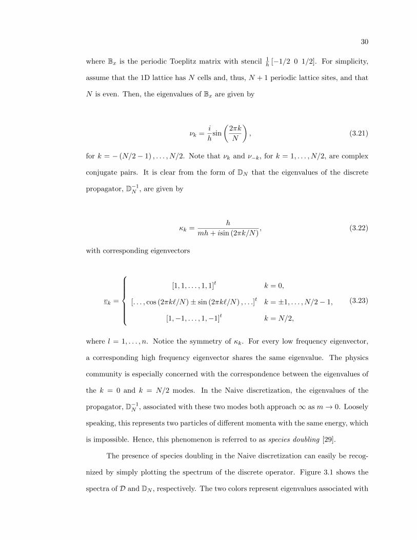
nized by simply plotting the spectrum of the discrete operator. Figure 3.1 shows the

spectra of D and DN , respectively. The two colors represent eigenvalues associated with

31

low and high frequency modes. Notice that, in the spectrum of the continuum operator,

the high frequency eigenvalues continue to grow in absolute value, while, in the Naive

operator, the high frequency modes double back over the low frequency modes.

0 0.1−100

−80

−60

−40

−20

0

20

40

60

80

100

(a) Spectrum of D0 0.05 0.1 0.15 0.2

−40

−30

−20

−10

0

10

20

30

40

(b) Spectrum of DN

Figure 3.1: The spectrum of the 1D, gauge free continuum Schwinger operator, D, andthe Naive discrete operator, DN , respectively, with m = 0.1 and N = 32. Red and bluedots indicate low and high frequency modes, respectively.

In the applied mathematics community, doubling is known as a red-black insta-

bility. There are a number of successful remedies [50]. However, the issue is not only

removal of the spurious high frequency components in the discrete solution, but overall

accuracy of the discretization process. The addition of the complex gauge field further

complicates the situation. The traditional remedy in the physics community is to add

an artificial stabilization term to DN , which we demonstrate below.

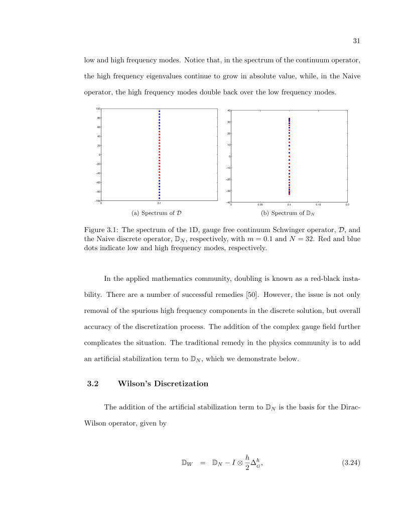
3.2 Wilson’s Discretization

The addition of the artificial stabilization term to DN is the basis for the Dirac-

Wilson operator, given by

DW = DN − I ⊗h

2∆hG, (3.24)

32

where ∆hG

is a discretization of the so-called Gauge Laplacian operator. The stencil for

the Gauge Laplacian is given by

∆hG

=1

h2

eiθj,k+1/2

e−iθj−1/2,k −4 eiθj+1/2,k

e−iθj,k−1/2

. (3.25)

Notice that, in the gauge-free case, ∆hG

coincides with the usual finite difference dis-

cretization of the Laplace operator. In matrix form, the Dirac-Wilson operator is given

by

DW =

−h2 ∆h

G+mI ∇hx − i∇hy

∇hx + i∇hy −h2 ∆h

G+mI

. (3.26)

The addition of the Gauge Laplacian ensures that each unknown is self-connected,

even in the massless case. Thus, the problem of species doubling is averted, because

red-black instability no longer exists. In addition to the centered differences of the first-

order terms, the diffusion-like terms now couple each component of the discrete fermion

field to its nearest neighbors. This can be seen by again looking at the spectrum of the

discrete operator in the 1D gauge free case. Then,

DW =

12H +mI Bx

Bx 12H +mI

, (3.27)

where Bx again has the periodic Toeplitz matrix with stencil 1h [−1/2 0 1/2], and H

is the periodic Toeplitz matrix constructed via the 3-point, periodic, Laplacian stencil

1h [−1 2 − 1]. Note that H and Bx both have eigenvectors corresponding to the discrete

Fourier modes defined in (3.23). Again, assume that the 1D lattice has N cells and that

33

N is even. Then, the eigenvalues of BN are again given by νk as defined in (3.21). The

eigenvalues of H are given by

αk =2

h

[1− cos

(2πk

N

)]. (3.28)

Consequently, the eigenvalues of the Dirac-Wilson propagator, D−1W , are given by

λk =

[m+

1

2αk ±

1

hνk

]−1

=

[m+

1

h

1− cos

(2πk

N

)± i sin

(2πk

N

)]−1

,

Note that, in this formulation, the eigenvalue corresponding to the lowest frequency

mode, that is, λ0, does approach ∞ as m→ 0, but the eigenvalue corresponding to the

highest frequency, that is, λN/2, now approaches h. Thus, the Dirac-Wilson operator

does not suffer from species doubling.

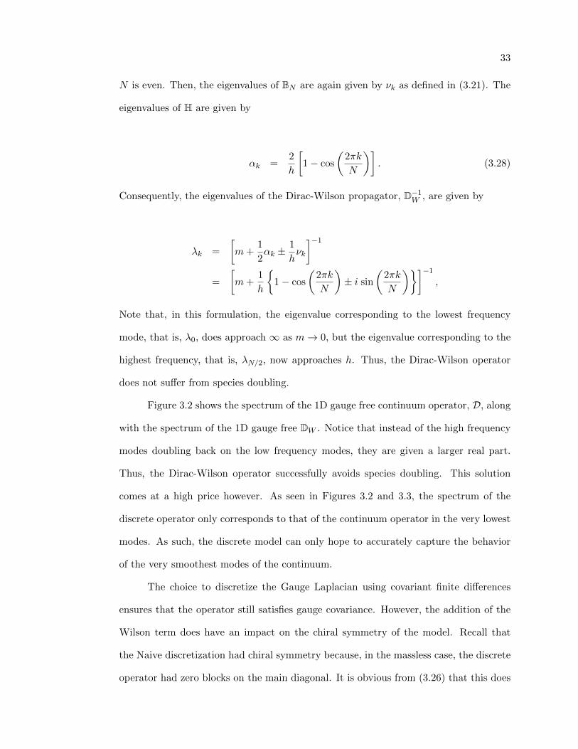
Figure 3.2 shows the spectrum of the 1D gauge free continuum operator, D, along

with the spectrum of the 1D gauge free DW . Notice that instead of the high frequency

modes doubling back on the low frequency modes, they are given a larger real part.

Thus, the Dirac-Wilson operator successfully avoids species doubling. This solution

comes at a high price however. As seen in Figures 3.2 and 3.3, the spectrum of the

discrete operator only corresponds to that of the continuum operator in the very lowest

modes. As such, the discrete model can only hope to accurately capture the behavior

of the very smoothest modes of the continuum.

The choice to discretize the Gauge Laplacian using covariant finite differences

ensures that the operator still satisfies gauge covariance. However, the addition of the

Wilson term does have an impact on the chiral symmetry of the model. Recall that

the Naive discretization had chiral symmetry because, in the massless case, the discrete

operator had zero blocks on the main diagonal. It is obvious from (3.26) that this does

34

0 0.1−100

−80

−60

−40

−20

0

20

40

60

80

100

(a) Spectrum of D0.1 35 70

−40

−20

0

20

40

(b) Spectrum of DW

Figure 3.2: The spectrum of the 1D, gauge free, continuum Schwinger operator, D, andDirac-Wilson operator, DW , respectively, with m = .01 and N = 32. Red and blue dotsindicate low and high frequency modes, respectively.

0 0.5 1 1.5 2 2.5 3 3.5 4 4.5−1.5

−1

−0.5

0

0.5

1

1.5

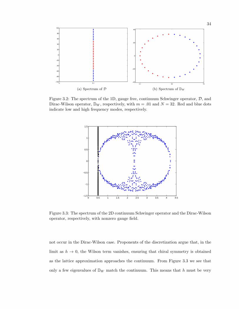
Figure 3.3: The spectrum of the 2D continuum Schwinger operator and the Dirac-Wilsonoperator, respectively, with nonzero gauge field.

not occur in the Dirac-Wilson case. Proponents of the discretization argue that, in the

limit as h → 0, the Wilson term vanishes, ensuring that chiral symmetry is obtained

as the lattice approximation approaches the continuum. From Figure 3.3 we see that

only a few eigenvalues of DW match the continuum. This means that h must be very

35

small in order for many of the discrete eigenvector-eigenvalue pairs to agree with the

continuum.

Chapter 4

The Least-Squares Finite Element Method

The least-squares finite element methodology has been employed in many in-

stances to overcome the shortcomings of the standard Galerkin finite element method

applied to nonsymmetric systems of first-order PDEs. Applying the Galerkin methodol-

ogy to such systems often leads to significant deficiencies. One such deficiency resulting

from the Galerkin discretization of first-order operators is red-black instability, or, in

the context of lattice gauge theory, species doubling. Many stabilization strategies exist

for this difficulty including adding artificial diffusion to the governing equations (as in

Wilson’s discretization) and employing nonsymmetric discretization techniques, such as

upwinding [50]. It has been demonstrated that the former strategy, in the context of

covariant finite differences, can do serious damage to the spectrum of the discrete oper-

ator. The latter strategy is immediately discounted by the physics community because

it leads to lattice actions that give an artificial preference to one spatial direction over

another.

Initially applied to first-order system formulations of convection diffusion prob-

lems, the least-squares methodology has since been successfully applied to problems in

fluid flow (Navier-Stokes) [6], [7], electromagnetism (Maxwell’s equations) [41], neutron

transport [3], [40], and plasma physics (magnetohydrodynamics) [1]. In general, the

method formulates the solution of a system of first-order PDEs in terms of a minimiza-

tion principle in an infinite dimensional Hilbert space. Then, restricting the resulting

37

weak form to a finite dimensional space results in a symmetric positive semidefinite

system of linear equations.

In this section, we consider a general system of first-order, linear, PDEs of the

form Lψ = f . Here, L : V 7→(L2)r

, where r is the number of equations in the system

and V ⊂(H1)r

is a Hilbert space over the complex numbers with appropriate boundary

conditions. Let R be the problem domain and define the following norms and their

associated spaces:

‖ψ‖0 =

(∫R|ψ(x)|2dx

)1/2

,

L2 (R) = ψ : ‖ψ‖0 <∞ ,

‖ψ‖1 =(‖ψ‖20 + ‖∇ψ‖20

)1/2,

H1 (R) = ψ : ‖ψ‖1 <∞ .

The linear system, Lψ = f , is then recast as a minimization problem according to

ψ = arg minϕ∈V

G (ϕ, f) := arg minϕ∈V‖Lϕ− f‖20, (4.1)

where ψ is the solution in V. If ψ is the minimizer in (4.1), then clearly ψ satisfies

G′ (ψ) [v] = 0, (4.2)

where G′ (ψ) [v] is the Frechet derivative of G, in the direction of v ∈ V, evaluated at

ψ. Then, (4.2) implies that (4.1) can be cast as the solution of the weak form

38

Find ψ ∈ V s.t. 〈Lψ,Lv〉 = 〈f,Lv〉 ∀v ∈ V, (4.3)

where 〈 · , · 〉 is the L2 inner product. It is worth noticing that, for sufficiently smooth

ψ and f , (4.3) is equivalent to

Find ψ ∈ V s.t. 〈L∗Lψ, v〉 = 〈L∗f, v〉 ∀v ∈ V, (4.4)

where L∗ represents the formal adjoint of L. This is the same weak form that would

result from applying a Ritz-Galerkin method to L∗Lψ = L∗f . Note that this is simply

the continuum normal equations of the original problem, Lψ = f . It is common then,

to look at the formal normal, L∗L, for insight into the nature of the linear system that

results from the least-squares discretization. Note that, in general, L∗L is self-adjoint

and nonnegative, a quality that the continuum Dirac operator does not have.

A desirable property of the least-squares functional, G, defined in (4.1), is that

G (ψ, 0) is elliptic with respect to some norm.

Definition 4.0.1. Quadratic functional F is said to be elliptic on V with respect to

norm ‖ · ‖ if there exists positive constants c and C, independent of ψ, such that

c‖ψ‖2 < F (ψ) < C‖ψ‖2 ∀ψ ∈ V. (4.5)

The left-hand inequality is known as the coercivity condition. The right-hand inequality

is known as the continuity condition.

If functional G is elliptic, then the minimization principle given in (4.1), and by exten-

sion, the weak form given in (4.3), has a unique solution on V.

To obtain a discrete linear system that approximates the continuum equations we

restrict V to a suitable finite-dimensional subspace, Vh ⊂ V, where Vh = span φj for

some set of basis functions φj. Then, the weak form in (4.3) becomes

39

Find ψh ∈ Vh s.t.⟨Lψh,Lvh

⟩=

⟨f,Lvh

⟩∀vh ∈ Vh. (4.6)

This discrete weak form is equivalent to the system of linear equations

Aψ = f, (4.7)

where

[A]jk = 〈Lφk,Lφj〉 , (4.8)[f]j

= 〈f,Lφj〉 , (4.9)

and the discrete solution, ψ, is related to the finite element solution, ψh, according to

ψh =∑j

ψjφj . (4.10)

It is easy to see from (4.8) that the resulting matrix operator, A, is Hermitian positive

semidefinite. Finally, if G (ψ, 0) can be shown to be elliptic with respect to the H1 norm,

an optimal multilevel iterative method exists that can efficiently solve the resulting linear

system, given in (4.7) [54].

Chapter 5

Least-Squares Finite Elements for the Schwinger Model

This chapter introduces a discretization of the 2D Schwinger model using least-

squares finite elements. Since this leads to a discrete solution process that is not au-

tomatically gauge covariant, the method is then modified using a process called gauge

fixing. The resulting process is shown to satisfy discrete gauge covariance and chiral

symmetry without suffering from species doubling. Next, H1-ellipticity of the least-

squares functional is demonstrated, the implications of which are discussed for the

physical properties of the discrete operator as well as its solution by multilevel itera-

tive methods. Finally, numerical experiments are carried out to test the effectiveness

of algebraic multigrid (AMG) and adaptive smoothed aggregation multigrid (αSA) as

preconditioners for solving the system of linear equations. The results show that the

discrete least-squares operator can be solved effectively by a multilevel method. Fur-

thermore, AMG and αSA, applied to the least-squares system, do not suffer from critical

slowing down. Finally, the performance of AMG as a preconditioner for the least-squares

operator is compared with the performance of αSA as a preconditioner for the solution

of the Dirac-Wilson operator. We find that the least-squares operator can be inverted

roughly six times as fast as the Dirac-Wilson operator.

41

5.1 The Least-Squares Discretization

The goal of this chapter is to discretize the 2D Schwinger model using least-

squares finite elements. The governing equations are reiterated here for convenience:

mI ∇x − i∇y

∇x + i∇y mI

ψR

ψL

=

fR

fL

in R, (5.1)

ψ(0, y) = ψ(1, y) ∀y ∈ (0, 1),

ψ(x, 0) = ψ(x, 1) ∀x ∈ (0, 1),

Let VR and VC be spaces of continuous, periodic, real- and complex-valued functions,

respectively. The solution of (5.1) can be reformulated in terms of a minimization

principle:

ψ = arg minϕ∈V2

C

G (ϕ,A; f) := arg minϕ∈V2

C

‖Dϕ− f‖20. (5.2)

The decision to cast the minimization problem in terms of the L2-norm requires that

(Dϕ− f) ∈[L2 (R)

]2. It is sufficient to require that the components of the source

term, fR and fL , belong to L2 (R), the components of the fermion field, ψR and ψL ,

belong to H1 (R), and the components of the gauge field, A1 and A2, be essentially

bounded and belong to L∞ (R). Then, given the restrictions that ψ and A be periodic,

let VC be the space of periodic, complex-valued functions in H1 (R), and let VR be the

space of periodic, real-valued, essentially bounded functions in L∞ (R). Furthermore,

if A ∈ [L∞ (R)]2, and A has the Helmholtz decomposition A = ∇⊥u +∇v + k, where

u and v are periodic, then u and v must belong to some space WR ⊂ W∞1 (R), where

W∞1 (R) is the space of periodic, real-valued functions belonging to L∞ (R) and whose

partial derivatives belong to L∞ (R) as well. WR, then, is the subspace of W∞1 (R)

42

consisting of periodic, real-valued functions [17].

Equation (5.2) is equivalent to the weak form

Find ψ ∈ V2C s.t. 〈Dψ,Dv〉 = 〈f,Dv〉 ∀v ∈ V2

C . (5.3)

The formal normal, D∗D, in this case appears as

D∗D =

mI −∇x + i∇y

−∇x − i∇y mI

mI ∇x − i∇y

∇x + i∇y mI

=

m2I −∇2x −∇2

y − i [∇x,∇y] 0

0 m2I −∇2x −∇2

y − i [∇y,∇x]

.Thus, the discrete operator that the least-squares methodology produces has uncoupled

Laplacian-like terms on the main diagonal. Note that the term ∇2x +∇2

y is the contin-

uum version of the gauge Laplacian discussed previously. Though these are not sim-

ple constant-coefficient operators (because they include the random background fields),

their Hermitian positive semidefinite scalar character should lend themselves to efficient

solution by multilevel methods.

The finite element solution is obtained by restricting the minimization problem in

(5.2), and, thus, the weak form in (5.3), to a finite-dimensional space, VhC ⊂ VC . Then,

the finite-element approximation to the solution, ψh, must satisfy the weak form

Find ψh ∈(VhC)2

s.t.⟨Dψh,Dvh

⟩=

⟨f,Dvh

⟩∀vh ∈

(VhC)2. (5.4)

Note that D in (5.4) is the usual Dirac operator in the continuum. However, D depends

on the continuum gauge field, A. Since realistic continuum gauge data is not available

we must represent provided discrete gauge data by functions in the continuum. To do

this, we interpolate discrete gauge data to the continuum by replacing the continuum

43

gauge field, A, with finite element gauge data, Ah ∈ WhR ⊂ VR , thus making (5.4) well

defined. We assume that Ah is a good approximation to continuum gauge field, A,

such that ‖A − Ah‖∞ = O(h). Details of this process and the specific form of WhR are

provided below.

To compute the inner products in (5.4), a finite element basis is required for

fermion field ψh as well as the gauge field, Ah. In analogy to the nodal setting, each

elementary square on the lattice is represented by a quadrilateral finite element. Recall

that NC is the space of discrete complex-valued vectors, with values associated with the

lattice sites. We equate any discrete vector w =[wR, w

L

]t ∈ (NC)2 with the piecewise

bilinear function wh =[whR, wh

L

]t ∈ (VhC )2, where VhC = spanφjn2

j=1 is the space of

periodic piecewise bilinear finite element functions over the complex numbers. Here, φj

is the standard nodal basis function associated with lattice site xj . Then, naturally,

whR

=n2∑j=1

wRjφj ,

whL

=

n2∑j=1

wLjφj .

We wish to represent the discrete gauge field, A, in the continuum using a finite

element function. Recall that A = [A1, A2]t belongs to E , the space of discrete real-

valued vectors, with values associated with the lattice links. Gauge data, A1 and A2,

define values on the horizontal and vertical lattice links, respectively. We associate

any A ∈ E with Ah =[Ah1 , A

h2

]t ∈ WhR, where Ah is chosen to exactly interpolate the

discrete gauge data on the centers of lattice links. To define Ah and WhR precisely we

first consider a Helmholtz decomposition of the discrete gauge field:

A =

A1

A2

=

C1 G1

C2 G2

u

v

+

k1

k2

(5.5)

44

where C =[Ct1 Ct2

]tand G =

[Gt

1 Gt2

]tare discrete representations of the curl and

gradient operators, respectively. The specific form of C and G will be described below.

Vectors v and u are real-valued and are associated with the sites of the standard lattice

and the cell-centered lattice, respectively. Then u, v ∈ NR . Note that each row in (5.5)

corresponds to gauge data on a link on the standard lattice, with the first block row

corresponding to the horizontal links and the second block row corresponding to the

vertical links. The rows of the matrix in (5.6), denoted alternatively by [C G], are

defined by the relationship between the individual lattice links, and their contributions

from u and v values on adjoining lattice sites. This relationship is illustrated in Figure

5.1. From this, we see that the rows of matrices G and C are defined by the appropriate

centered differences that map values of v and u at sites on the standard and cell-centered

lattice, respectively, to values on the links of the standard lattice.

−1 1

h

1

h

h

h

−1

−1 1

h

1

h

h

h

−1

Figure 5.1: Contributions of u and v to discrete gauge data on a horizontal lattice link(left) and a vertical lattice link (right). and represent sites on the standard andcell-centered lattice, respectively. Solid and dashed lines represent links on the standardand cell-centered lattice, respectively.

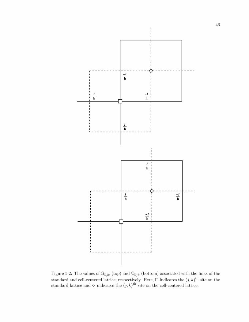
The columns of G and C are defined by their action on canonical basis functions asso-

ciated with the standard and cell-centered lattice, respectively. Let ejk be the vector,

defined on the standard lattice, with value 1 at the (j, k)th lattice site and zero at all

45

other sites. Similarly, let εjk be the vector, defined on the cell-centered lattice, with

value 1 at the (j, k)th cell-centered lattice site and zero at all other sites. Here, we use

the convention that the (j, k)th site on the cell-centered lattice is located at the center

of the cell with the (j, k)th standard lattice site in its lower left corner. Figure 5.2 shows

the values of Gejk and Cεjk on the appropriate lattice links.

In the following theorem, we establish the existence and uniqueness of the decom-

position defined in (5.5).

Theorem 5.1.1. For discrete gauge field A ∈ E, defined on an (N + 1) × (N + 1)

periodic lattice, there exist unique vectors, v and u, defined on the standard and cell-

centered lattice, respectively, such that

A = Cu+ Gv +

k1

k2

, (5.6)

and

∑jk

ujk =∑jk

vjk = 0,

for some constants, k1 and k2.

Proof. Note that the (N + 1) × (N + 1) periodic lattice has 2N2 distinct lattice links.

Thus, A ∈ R2N2. We begin by showing that, for any discrete gauge field, A,

A ∈ E = Range (C)⊕ Range (G)⊕K, (5.7)

where K is the space of vectors that are of a constant value on the horizontal lattice

links, and of a (possibly different) constant value on the vertical lattice links. Thus,

dim (K) = 2.

46

h

1

h

−1

h

−1

h

1

h

−1

h

−1

h

1

h

1

Figure 5.2: The values of Gejk (top) and Cεjk (bottom) associated with the links of the

standard and cell-centered lattice, respectively. Here, indicates the (j, k)th site on thestandard lattice and indicates the (j, k)th site on the cell-centered lattice.

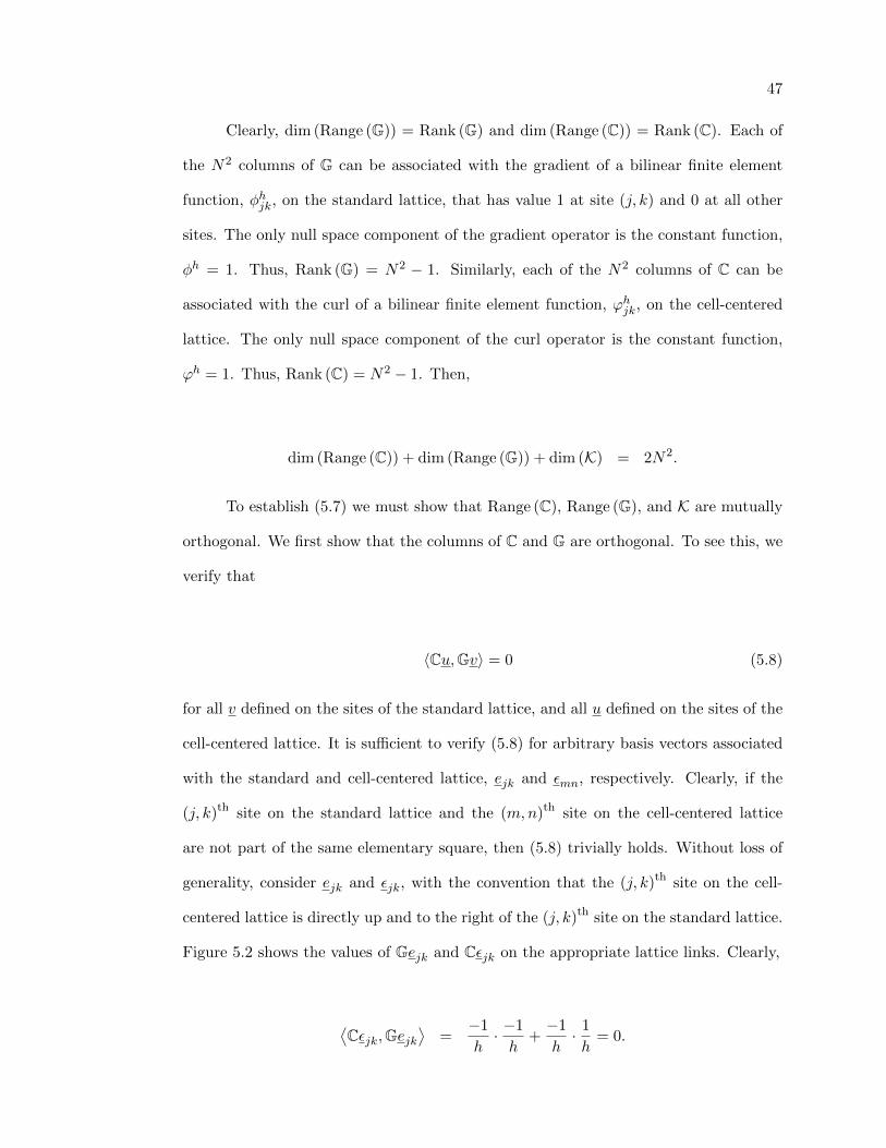
47

Clearly, dim (Range (G)) = Rank (G) and dim (Range (C)) = Rank (C). Each of

the N2 columns of G can be associated with the gradient of a bilinear finite element

function, φhjk, on the standard lattice, that has value 1 at site (j, k) and 0 at all other

sites. The only null space component of the gradient operator is the constant function,

φh = 1. Thus, Rank (G) = N2 − 1. Similarly, each of the N2 columns of C can be

associated with the curl of a bilinear finite element function, ϕhjk, on the cell-centered

lattice. The only null space component of the curl operator is the constant function,

ϕh = 1. Thus, Rank (C) = N2 − 1. Then,

dim (Range (C)) + dim (Range (G)) + dim (K) = 2N2.

To establish (5.7) we must show that Range (C), Range (G), and K are mutually

orthogonal. We first show that the columns of C and G are orthogonal. To see this, we

verify that

〈Cu,Gv〉 = 0 (5.8)

for all v defined on the sites of the standard lattice, and all u defined on the sites of the

cell-centered lattice. It is sufficient to verify (5.8) for arbitrary basis vectors associated

with the standard and cell-centered lattice, ejk and εmn, respectively. Clearly, if the

(j, k)th site on the standard lattice and the (m,n)th site on the cell-centered lattice

are not part of the same elementary square, then (5.8) trivially holds. Without loss of

generality, consider ejk and εjk, with the convention that the (j, k)th site on the cell-

centered lattice is directly up and to the right of the (j, k)th site on the standard lattice.

Figure 5.2 shows the values of Gejk and Cεjk on the appropriate lattice links. Clearly,

⟨Cεjk,Gejk

⟩=−1

h· −1

h+−1

h· 1

h= 0.

48

Thus, (5.8) holds for all v on the standard lattice and u on the cell-centered lattice, and

the columns of C and G are orthogonal.

Next, we observe that

〈Cu, k〉 = 〈Gv, k〉 = 0, (5.9)

for all v on the standard lattice, u on the cell-centered lattice, and arbitrary constant

vector k =[kt1 kt2

]tdefined on the lattice links. Again, it is sufficient to verify (5.9) for

arbitrary canonical basis vectors, ejk and εjk. From the representation of Gejk and Cεjk

in Figure 5.2, it is easy to see that multiplying horizontal link values by k1 and vertical

link values by k2, and then summing the results establishes (5.9). Thus, Range (C) and

Range (G) are orthogonal to K. This establishes that any discrete gauge field, A, has a

decomposition of the form (5.6).

Under the current assumptions, the decomposition defined in (5.6) is not unique.

Since constant vectors are in the null space of both C and G, any u and u, and any

v and v, that differ by only a constant, will produce the same A. To remedy this, we

require that the entries of u and v individually sum to zero. That is, we require that

∑jk

ujk =∑jk

vjk = 0.

Under these conditions, the decomposition defined in (5.6) is unique, and the proof is

complete.

The decomposition of E , given in (5.7), suggests a method of computing v and u,

for any gauge field, A. Specifically, u is the orthogonal projection of A onto the space of

vectors in Range (C) whose entries sum to zero. Likewise, v is the orthogonal projection

49

of A onto the space of vectors in Range (G) whose entries sum to zero. Thus, u and v

are the solutions to the following sets of normal equations:

CtCu = CtA, (5.10)

GtGv = GtA, (5.11)

where C and G are versions of C and G modified to enforce the condition that the

entries of u and v sum to zero. The matrices on the left-hand side of (5.10) and (5.11)

are similar to constant coefficient Poisson operators discretized via finite differences.

Thus, they can easily be inverted using standard methods. Finally, constants k1 and k2

are found by computing

k1

k2

= A− Cu−Gv. (5.12)

The development of the Helmholtz decomposition of the discrete gauge field leads

us to a convenient representation of the discrete gauge data by a finite element function,

Ah. Recall that we related the action of G and C on discrete vectors to the application

of the gradient and curl operators to bilinear finite element functions defined on the

standard and cell-centered lattice, respectively. Then, Ah can be defined in terms of a

continuum Helmholtz decomposition involving bilinear finite element functions vh and

uh defined on the standard and cell centered lattice, respectively, whose entries at lattice

sites correspond exactly with the discrete values of v and u. This decomposition is,

Ah = ∇⊥uh +∇vh + k. (5.13)

The definition of vh as a bilinear finite element function on the standard lattice implies

that the gradient portion of the gauge field, ∇vh, belongs to Whv , the Nedelec space

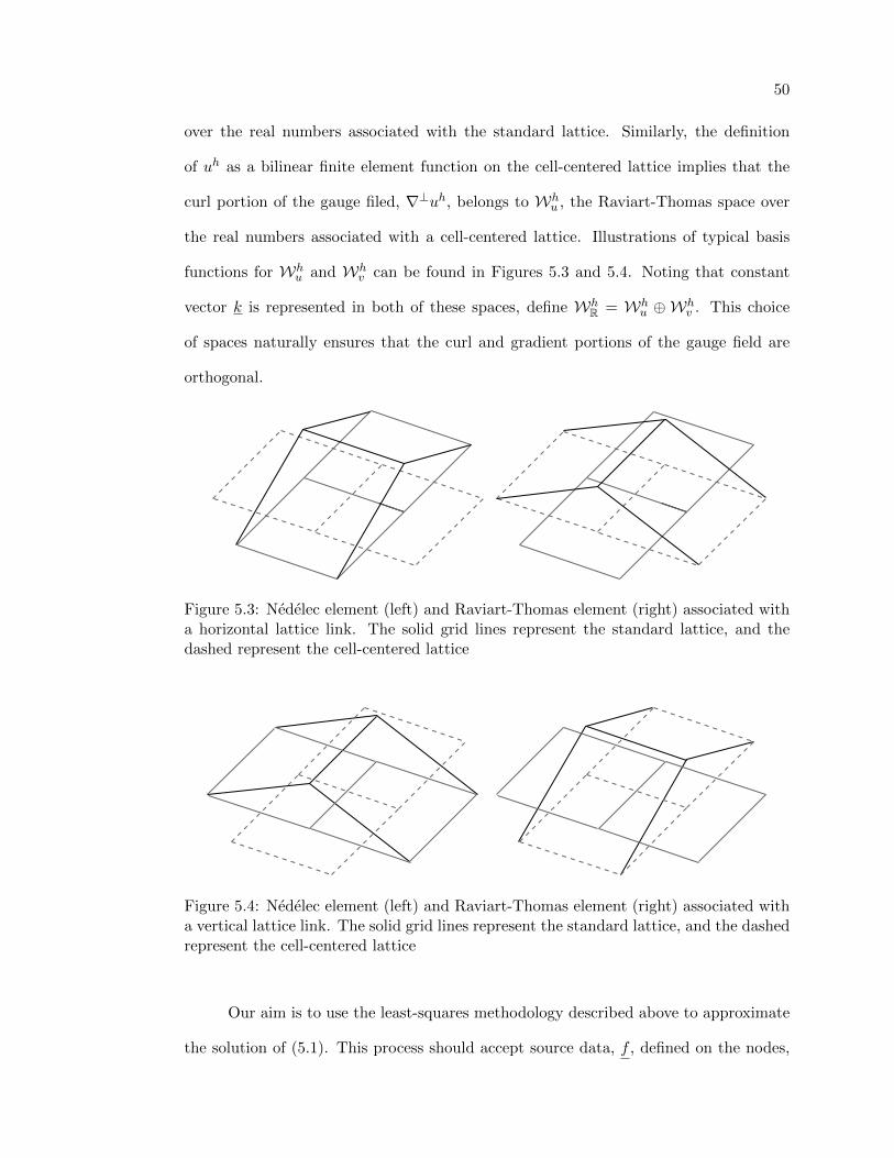
50

over the real numbers associated with the standard lattice. Similarly, the definition

of uh as a bilinear finite element function on the cell-centered lattice implies that the

curl portion of the gauge filed, ∇⊥uh, belongs to Whu , the Raviart-Thomas space over

the real numbers associated with a cell-centered lattice. Illustrations of typical basis

functions for Whu and Wh

v can be found in Figures 5.3 and 5.4. Noting that constant

vector k is represented in both of these spaces, define WhR = Wh

u ⊕ Whv . This choice

of spaces naturally ensures that the curl and gradient portions of the gauge field are

orthogonal.

Figure 5.3: Nedelec element (left) and Raviart-Thomas element (right) associated witha horizontal lattice link. The solid grid lines represent the standard lattice, and thedashed represent the cell-centered lattice

Figure 5.4: Nedelec element (left) and Raviart-Thomas element (right) associated witha vertical lattice link. The solid grid lines represent the standard lattice, and the dashedrepresent the cell-centered lattice

Our aim is to use the least-squares methodology described above to approximate

the solution of (5.1). This process should accept source data, f , defined on the nodes,

51

and gauge field data A, prescribed on the lattice links, and return the discrete wave-

function, ψ, defined at the nodes. This is accomplished by mapping f and A into their

respective finite element spaces, solving the weak formulation (5.4), and mapping the

resulting finite element solution back to N 2C . This process is summarized in Algorithm

5.1.

ALGORITHM 5.1: Least-Squares Dirac Solve

Input: Gauge field A, source term f .

Output: Wavefunction ψ.

1. Map A 7→ Ah ∈ WhR.

2. Map f 7→ fh ∈(VhC)2

.

3. Find ψh ∈(VhC)2

s.t.⟨Dψh,Dvh

⟩=⟨fh,Dvh

⟩∀vh ∈

(VhC)2

,

where D = D(Ah).

4. Map ψh 7→ ψ ∈ N 2C .

5.1.1 Gauge Covariance

A little reflection on the property of gauge covariance of the fermion propagator

in the continuum leads to a test for covariance of the discrete solution process. Let

ω (x, y) be some periodic function and define

Tω =

eiω(x,y) 0

0 eiω(x,y)

.Note that Tω is a unitary operator. Consider the following related Dirac equations in

the continuum:

52

D (A)ψ = f, (5.14)

D (A−∇ω) ψ = T ∗ω f, (5.15)

where T ∗ω is the formal adjoint of Tω. It is easy to see, by the principle of gauge

covariance, that ψ and ψ are related according to

ψ = Tω ψ.

Transferring these facts to the discrete lattice, let ω be the usual vector of values of

ω (x, y) evaluated at the lattice sites. Let the discrete gauge transformation, Ωω, and

the associated matrix, Tω, be as defined in (3.10) and (3.11), respectively. Consider,

now, the discrete analogues of (5.14) and (5.15):

D (A)ψ = f, (5.16)

D (A−Gω) ψ = T∗ω f. (5.17)

Note that (5.16) and (5.17) are simply the discrete Dirac operator constructed using

two sets of gauge data, A and A, and two sets of source data, f and f , related according

to

A = A−Gω, (5.18)

f = T∗ω f. (5.19)

Then, given these two sets of inputs, any discrete solution process should yield solution

vectors, ψ and ψ, such that

ψ = Tω ψ.

53

Unfortunately, Algorithm 5.1 does not pass this test. To see this, first consider

the test for gauge covariance in the continuum. Suppose the weak form in Algorithm

5.1 is applied to both sets of gauge and source data, but on the entire continuum space

V2C , rather than

(VhC)2

. Then, solutions ψ and ψ must satisfy, for all w ∈ V2C ,

〈D (A)ψ,D (A)w〉 = 〈f,D (A)w〉 , (5.20)⟨D (A−∇ω) ψ,D (A−∇ω)w

⟩=⟨f ,D (A−∇ω)w

⟩, (5.21)

respectively. Setting ψ = T ∗ω ξ, f = T ∗ω f , and w = T ∗ω v, (5.21) becomes

〈D (A−∇ω)T ∗ω ξ,D (A−∇ω)T ∗ω v〉 = 〈T ∗ω f,D (A−∇ω)T ∗ω v〉 . (5.22)

By gauge covariance, (5.22) is equivalent to

〈T ∗ω D (A) ξ, T ∗ω D (A) v〉 = 〈T ∗ω f, T ∗ω D (A) v〉 . (5.23)

Finally, canceling the gauge transformations, (5.23) becomes

〈D (A) ξ,D (A) v〉 = 〈f,D (A) v〉 . (5.24)

Clearly, (5.20) and (5.24) are equivalent. Thus, ξ = ψ and, as a result, ψ = Tωψ,

as desired. This is not surprising since the continuum formulation of the Dirac equa-

tion satisfies gauge covariance. Then, restricting the associated weak forms to their

respective finite element spaces suggests a test for the gauge covariance of Algorithm

5.1.

54

Consider discrete gauge fields, A and A, and source terms, f and f , related

according to (5.18) and (5.19), respectively. Then, for the two data sets, the equalities

in the weak forms in Algorithm 5.1 become, for all wh ∈(VhC)2

,

⟨D(Ah)ψh,D(Ah)wh

⟩=⟨fh,D(Ah)wh

⟩, (5.25)⟨

D(Ah −∇ωh)ψ h,D(Ah −∇ωh)wh⟩

=⟨f h,D(Ah −∇ωh)wh

⟩, (5.26)

where ωh is the projection of ω into(VhR)2

and f h is the L2-projection of T∗ω f into(VhC)2

. Proceeding as before, set ψ h = T ∗ωhξh and wh = T ∗

ωhvh. Then, (5.26) becomes

⟨D(Ah −∇ωh)T ∗ωh ξ

h,D(Ah −∇ωh)T ∗ωh vh⟩

=⟨f h,D(Ah −∇ωh)T ∗ωh v

h⟩. (5.27)

Again, by gauge covariance of D, (5.27) is equivalent to

⟨T ∗ωhD(Ah)ξh, T ∗ωhD(Ah)vh

⟩=⟨f h, T ∗ωhD(Ah)vh

⟩. (5.28)

Moving the T ∗ωh

to the other side of the inner product yields

⟨D(Ah)ξh,D(Ah)vh

⟩=⟨Tωh f

h,D(Ah)vh⟩

. (5.29)

Weak form (5.29) appears very similar to (5.25), except in the inner product on the

right-hand side. If it were the case that Tωh fh = fh, then Algorithm 5.1 would,

in fact, be gauge covariant. Unfortunately, since f h is obtained by first multiplying

(node-wise) the discrete entries of eiω and f , and then projecting the result into(VhC)2

,

this equality does not hold. Thus, Algorithm 5.1 is not gauge covariant. Luckily, this

problem can be circumvented using a process called gauge fixing.

Consider the continuum Dirac equation with gauge field A, given in (5.14). Write

the Helmholtz decomposition of the gauge field, A, as

55

A = A0 +∇v,

where

A0 = ∇⊥u+ k,

for periodic functions u and v and constant vector k. Note then that A0 is divergence-

free. Equation (5.14) becomes

D (A0 +∇v)ψ = f,

to which the solution is

ψ = [D (A0 +∇v)]−1 f.

Rewriting the source function as

f = Tv g,

for some g ∈ V2C , (5.30) becomes

ψ = [D (A0 +∇v)]−1 Tv g.

But, from gauge covariance of the propagator,

ψ = Tv [D (A0)]−1 g,

56

implying

ψ = Tv [D (A0)]−1 T ∗v f.

Now, consider the continuum equation with modified input data, (5.15). In this case,

the Helmholtz decomposition of A is

A = A0 +∇ (v − ω) ,

and the Dirac equation becomes

D (A0 +∇ (v − ω)) ψ = f .

Writing the source term as f = Tv−ω g, the solution becomes

ψ = [D (A0 +∇ (v − ω))]−1 Tv−ω g.

Again, by gauge covariance, the solution becomes

ψ = Tv−ω [D (A0)]−1 g,

implying

ψ = Tv−ω [D (A0)]−1 T ∗v−ωf

= Tω

Tv [D (A0)]−1 T ∗v f

.

Thus,

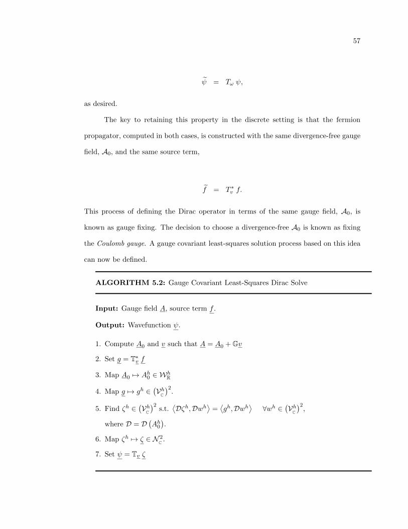
57

ψ = Tω ψ,

as desired.

The key to retaining this property in the discrete setting is that the fermion

propagator, computed in both cases, is constructed with the same divergence-free gauge

field, A0, and the same source term,

f = T ∗v f.

This process of defining the Dirac operator in terms of the same gauge field, A0, is

known as gauge fixing. The decision to choose a divergence-free A0 is known as fixing

the Coulomb gauge. A gauge covariant least-squares solution process based on this idea

can now be defined.

ALGORITHM 5.2: Gauge Covariant Least-Squares Dirac Solve

Input: Gauge field A, source term f .

Output: Wavefunction ψ.

1. Compute A0 and v such that A = A0 + Gv

2. Set g = T∗v f

3. Map A0 7→ Ah0 ∈ WhR

4. Map g 7→ gh ∈(VhC)2

.

5. Find ζh ∈(VhC)2

s.t.⟨Dζh,Dwh

⟩=⟨gh,Dwh

⟩∀wh ∈

(VhC)2

,

where D = D(Ah0).

6. Map ζh 7→ ζ ∈ N 2C .

7. Set ψ = Tv ζ

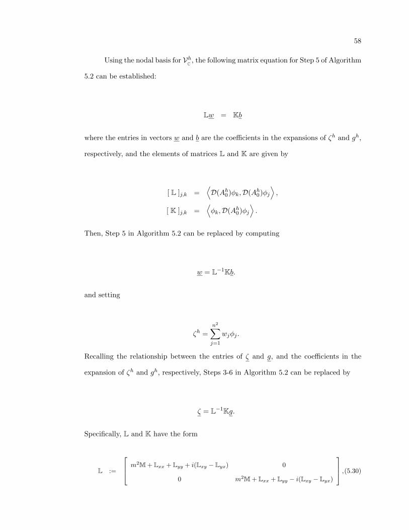
58

Using the nodal basis for VhC , the following matrix equation for Step 5 of Algorithm

5.2 can be established:

Lw = Kb

where the entries in vectors w and b are the coefficients in the expansions of ζh and gh,

respectively, and the elements of matrices L and K are given by

[ L ]j,k =⟨D(Ah0)φk,D(Ah0)φj

⟩,

[ K ]j,k =⟨φk,D(Ah0)φj

⟩.

Then, Step 5 in Algorithm 5.2 can be replaced by computing

w = L−1Kb.

and setting

ζh =n2∑j=1

wjφj .

Recalling the relationship between the entries of ζ and g, and the coefficients in the

expansion of ζh and gh, respectively, Steps 3-6 in Algorithm 5.2 can be replaced by

ζ = L−1Kg.

Specifically, L and K have the form

L :=

m2M + Lxx + Lyy + i(Lxy − Lyx) 0

0 m2M + Lxx + Lyy − i(Lxy − Lyx)

,(5.30)

59

K :=

mM Bx − iBy

Bx + iBy mM

, (5.31)

where

[ Lxx ]j,k =< ∇xφk,∇xφj > [ M ]j,k =< φk, φj >

[ Lyy ]j,k =< ∇yφk,∇yφj > [ Bx ]j,k =< φk,∇xφj >

[ Lxy ]j,k =< ∇xφk,∇yφj > [ By ]j,k =< φk,∇yφj >

[ Lyx ]j,k =< ∇yφk,∇xφj > .

It is important to notice that the covariant derivative operators, ∇x and ∇y, are con-

structed using the divergence-free gauge field, Ah0 . It is interesting to note the similarity

between the form of L given in (5.30) and the formal normal given in (5.4).

Matrix L is nonsingular, except in the case that m = 0 and the gauge field is an

exceptional configuration. To see this, note that, by construction,

‖Dψh‖20 =⟨Lψ,ψ

⟩l2, (5.32)

for any finite element fermion field ψh and its lattice counterpart ψ. From the discussion

of the spectrum of the continuum operator, D, in Section 2.1, it is clear from (5.32) that if

D is nonsingular, then L is positive definite, and thus nonsingular as well. Furthermore,

L is singular only when m = 0 and Ah0 is an exceptional configuration.

Note that K can be written as a sum of Hermitian and skew-Hermitian matrices

according to

K =

mM 0

0 mM

+

0 Bx − iBy

Bx + iBy 0

.

60

By construction, M is positive definite. Thus, if m > 0, then the first term in the

decomposition is also positive definite. This implies that K is positive definite, and thus

nonsingular. However, if Ah0 is an exceptional configuration, the skew-Hermitian term

is singular, and if m = 0, then K is singular as well.

Using the matrix representations described above, Algorithm 5.2 can be rewritten

completely in the discrete setting. This is summarized in Algorithm 5.3.

ALGORITHM 5.3: Discrete Gauge Covariant Least-Squares Dirac Solve

Input: Gauge field A, source term f .

Output: Wavefunction ψ.

1. Compute A0 and v such that A = A0 + Gv, where 〈A0,Gw〉 = 0 ∀w ∈ NC

2. Set g = T∗v f

3. Compute ζ = L−1Kg

4. Set ψ = Tv ζ

Combining Steps 2-4 in Algorithm 5.3 yields an expression for the discrete least-squares

propagator, hereafter denoted by D−1LS :

D−1LS = Tv L−1KT∗v. (5.33)

From (5.33), the least-squares representation of the Dirac operator is, naturally

DLS = Tv K−1LT∗v. (5.34)

Again, the operators given in (5.33) and (5.34) exist except in the case when m = 0 and

Ah0 is an exceptional configuration.

61

Finally, note that L and K are constructed using A0. An encouraging consequence

of constructing L based on A0 is that divergence-free gauge fields tend to be smoother

than general fields [10]. The decreased disorder in the background field makes L easier

to invert using a multilevel iterative method.

The following theorem establishes the discrete gauge covariance of Algorithm 5.3.

Theorem 5.1.2. The least-squares solution process defined in Algorithm 5.3 satisfies

discrete gauge covariance as described in Definition 3.1.1.

Proof. Recall that, given the least-squares propagator, D−1LS , and associated discrete

gauge transformation matrices, Ωω and Tω, there must exists a modified propagator,

denoted by D−1LS , such that

D−1LS Tω ξ = Tω D−1

LS ξ.

From (5.33),

D−1LS = Tv L−1KT∗v.

Then,

D−1LS Tω ξ = Tv L−1KT∗v Tω ξ

= Tω[Tv−ω L−1KT∗v−ω

]ξ.

Finally, defining D−1LS according to

D−1LS = Tv−ω L−1KT∗v−ω,

achieves the desired result.

62

5.1.2 Chiral Symmetry

Recall Definition 3.1.2 regarding the discrete chiral symmetry of a discrete Dirac

operator. Given λR and λL ∈ R, and associated transformation Λ, defined in (3.14), the

least-squares analogue of the Dirac operator, DLS , must satisfy

⟨Λξ,Γ1DLSΛξ

⟩=

⟨ξ,Γ1DLSξ

⟩, (5.35)

when m = 0. Recall from (5.34) that DLS is ill-posed in the massless case if the

discrete gauge field is an exceptional configuration, because K is not invertible. Even in

this case, the least-squares discretization should satisfy chiral symmetry. The following

lemma demonstrates that DLS satisfies an equivalent formulation of chiral symmetry.

Lemma 5.1.3. (Chiral symmetry for the discrete least-squares operator). Given any

λR , λL ∈ R, and any ψ, f ∈ N 2C such that

LT∗v ψ = KT∗v f

for m = 0, then

ψ = Λψ,

f = Γ1ΛΓ1f,

satisfy

LT∗v ψ = KT∗v f .

Proof. Recalling (5.30) and (5.31), it is easy to see that, in the massless case, L and K

are of the form

63

L =

L11 0

0 L22

,

K =

0 K12

K21 0

.Then, LT∗v and KT∗v appear as

LT∗v =

L11 Ω∗v 0

0 L22 Ω∗v

, (5.36)

KT∗v =

0 K12 Ω∗v

K21 Ω∗v 0

. (5.37)

The following can be deduced from the block structure of (5.36), and the constant nature

of the diagonal blocks of Λ:

LT∗v Λ = ΛLT∗v.

Then, from the block structure of (5.37) and the constant nature of Λ,

KT∗v Γ1 Λ Γ1 = Λ KT∗v.

Thus,

LT∗vψ = LT∗vΛψ

= ΛLT∗vψ,

and

64

KT∗v f = KT∗v Γ1 Λ Γ1f

= Λ KT∗v f,

which yields the result.

5.1.3 Species Doubling

From (5.30), the principle part of the main diagonal blocks of L is a 9-point

Laplacian-like stencil. Since this stencil connects each unknown to its nearest neighbors,

matrix L does not have red-black instability and, thus, the problem of species doubling

is averted. This is proved definitively now by examining the spectrum of the effective

least-squares operator DLS in the 1D gauge free case. In this instance,

L =

m2M + H 0

0 m2M + H

,

K =

mM Bx

Bx mM

,

Tv =

I 0

0 I

.where H, Bx, and M are periodic Toeplitz matrices with stencils 1

h [−1 2 − 1], [−1 0 1],

and h [1/6 2/3 1/6], respectively. The eigenvalues of M are given by

µk =h

3

[2 + cos

(2πk

n

)]. (5.38)

Then, the effective least-squares propagator is given by

65

D−1LS = L−1K, (5.39)

and its eigenvalues are given by

τk =mµk ± iνkm2µk + αk

. (5.40)

Substituting the expressions for µk, νk, and αk into (5.40) and simplifying gives

τk =m h2 [2 + cos (2πk/N)]± 3i h sin (2πk/N)

m2h2 [2 + cos (2πk/N)] + 6 [1− cos (2πk/N)], (5.41)

for k = −N/2+1, . . . , N/2. Recall from Chapter 3 that species doubling is present if the

eigenvalue associated with the highest frequency mode, τN/2, approaches∞ in the limit

as m→ 0. As expected, the eigenvalue associated with the lowest frequency mode, τ0,

approaches ∞ as m → 0. Then, setting k = N/2 and taking the limit to the massless

case, we see that τN/2 → 0, unlike in the naive propagator, where τN/2 → ∞. Thus,

the least-squares formulation for the 1D Dirac operator does not suffer from species

doubling. The generalization of this analysis to the 2D case is straightforward.

It is also easily verified that the effective least-squares operator does not suffer

from species doubling by looking at its spectrum graphically. The eigenvalues of the

1D, gauge-free operator are plotted in Figure 5.5. Again, low frequency eigenvalues are

given in red, and high frequency eigenvalues are given in blue. Notice that the high

frequency modes continue to grow in magnitude as the frequency increases, much like

the continuum Dirac operator. And, although the spectrum is not a perfect vertical

line in the complex plane, the low modes approximate the continuum much better than

those of the Dirac-Wilson operator.

Recall that, in the successful discretization of any PDE, the discrete operator

must do a good job of capturing the behavior of the continuum modes associated with

66

0.1 1 2−200

−100

0

100

200

Figure 5.5: The spectrum of the 1D, gauge free least-squares operator, DLS with m = 0.1and N = 32. Red and blue dots indicate low and high frequency modes, respectively.

eigenvalues of smallest modulus. In fact, the least-squares discretization does just this.

This point is further illustrated in Figure 5.6, where the lowest modes of the contin-

uum operator, the least-squares operator, and the Dirac-Wilson operator are displayed

together. Note that the least-squares operator represents the lowest modes of the con-

tinuum operator almost perfectly. On the other hand, only the single lowest mode of

the Dirac-Wilson operator comes close to the continuum spectrum.

Naturally, the eigenvectors associated with eigenvalues of small modulus in the

operator are associated with eigenvalues of large modulus in the propagator. It is

desirable, then, that the high frequency modes of the discrete propagator agree with

the high frequency modes of the continuum propagator. The upper end of the spectrum

is shown in Figure 5.7 for the continuum, least-squares, and Dirac-Wilson propagators.

Recall that the spectrum of the continuum propagator is on a circle in the complex

plane, with radius 12m , and centered on the real axis at 1

2m . Although the eigenvalues of

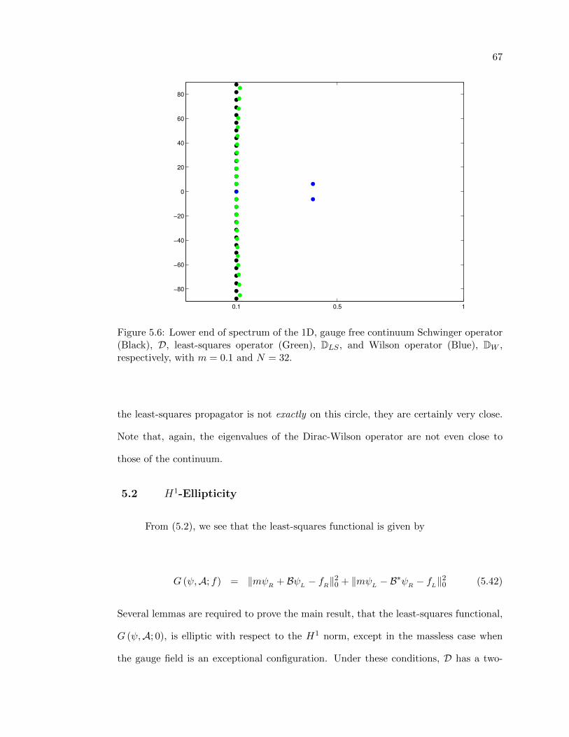
67

0.1 0.5 1

−80

−60

−40

−20

0

20

40

60

80

Figure 5.6: Lower end of spectrum of the 1D, gauge free continuum Schwinger operator(Black), D, least-squares operator (Green), DLS , and Wilson operator (Blue), DW ,respectively, with m = 0.1 and N = 32.

the least-squares propagator is not exactly on this circle, they are certainly very close.

Note that, again, the eigenvalues of the Dirac-Wilson operator are not even close to

those of the continuum.

5.2 H1-Ellipticity

From (5.2), we see that the least-squares functional is given by

G (ψ,A; f) = ‖mψR + BψL − fR‖20 + ‖mψL − B

∗ψR − fL‖20 (5.42)

Several lemmas are required to prove the main result, that the least-squares functional,

G (ψ,A; 0), is elliptic with respect to the H1 norm, except in the massless case when

the gauge field is an exceptional configuration. Under these conditions, D has a two-

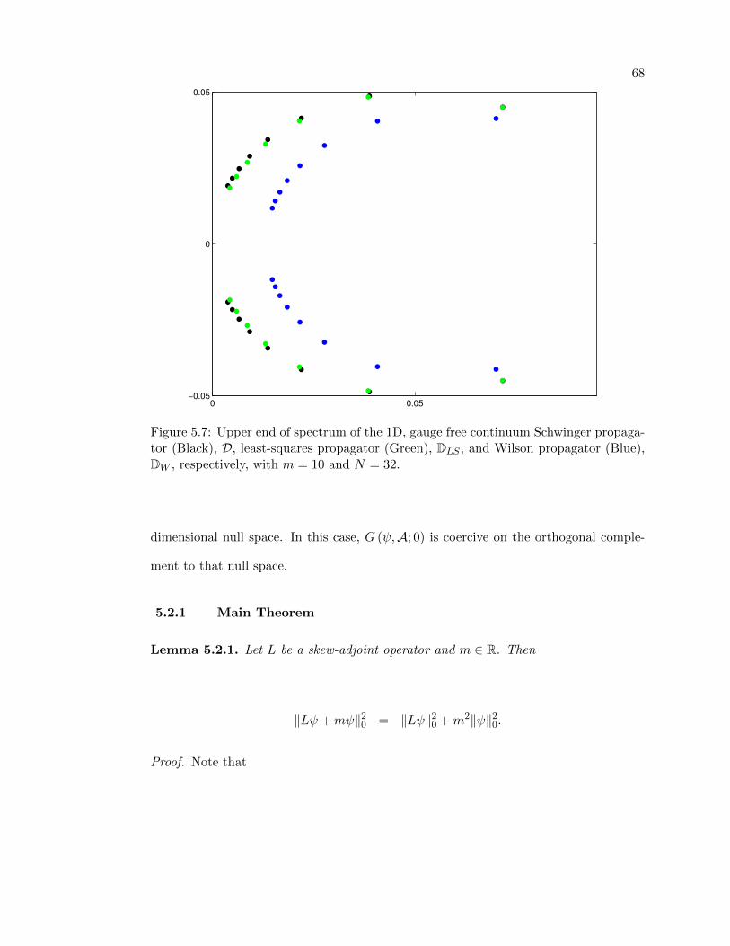
68

0 0.05−0.05

0

0.05

Figure 5.7: Upper end of spectrum of the 1D, gauge free continuum Schwinger propaga-tor (Black), D, least-squares propagator (Green), DLS , and Wilson propagator (Blue),DW , respectively, with m = 10 and N = 32.

dimensional null space. In this case, G (ψ,A; 0) is coercive on the orthogonal comple-

ment to that null space.

5.2.1 Main Theorem

Lemma 5.2.1. Let L be a skew-adjoint operator and m ∈ R. Then

‖Lψ +mψ‖20 = ‖Lψ‖20 +m2‖ψ‖20.

Proof. Note that

69

‖Lψ +mψ‖20 = 〈Lψ +mψ,Lψ +mψ〉

= 〈Lψ,Lψ〉+ 〈Lψ,mψ〉+ 〈mψ,Lψ〉+ 〈mψ,mψ〉

= 〈Lψ,Lψ〉+m 〈Lψ,ψ〉+m 〈L∗ψ,ψ〉+m2 〈ψ,ψ〉

= ‖Lψ‖20 +m 〈(L+ L∗)ψ,ψ〉+m2‖ψ‖20.

Then, noting that L∗ = −L, because L is skew-adjoint, proves the result.

Lemma 5.2.2. Let D0 be the massless Dirac operator and let U be a subspace of V2C . If

there exists some ck > 0 such that

‖D0ψ‖20 ≥ ck‖ψ‖21 ∀ψ ∈ U ,

then

‖Dψ‖20 ≥ ck‖ψ‖21 ∀ψ ∈ U .

Proof. Assume that D0 is coercive on U . That is, there exists ck > 0 such that

‖D0ψ‖20 ≥ ck‖ψ‖21 ∀ψ ∈ U . (5.43)

If m = 0, then the proof is complete. Thus, assume m > 0. Note that D0 is skew-adjoint.

Then, by Lemma 5.2.1,

‖ (D0 +mI)ψ‖20 = ‖D0ψ‖20 +m2‖ψ‖20.

Then

70

‖Dψ‖20 = ‖ (D0 +mI)ψ‖20

= ‖D0ψ‖20 +m2‖ψ‖20

≥ ck‖ψ‖21 +m2‖ψ‖20

≥ ck‖ψ‖21,

as desired.

Recall that gauge field A can be decomposed according to A = ∇⊥u+∇v+k. In

the alternate formulation of the Schwinger model, discussed in Section 2.2.3, we use a

transformation involving ez to remove the gauge field from the differential operators in

D, where z = u+ iv. Note that the choice of u, v ∈ WR ensures that z ∈ WC , the space

of periodic, complex-valued functions in W∞1 (R). This guarantees that ez is bounded

in the ∞-norm.

Lemma 5.2.3. Let UL be a subspace of VC, and define UL = ezUL and B = ezBke−z,

where B = ∇x − i∇y and Bk = (∂x − ik1)− i (∂y − ik2). If there exists ck > 0 such that

‖Bkξ‖20 ≥ ck‖ξ‖21 ∀ξ ∈ UL ,

then there exists cL > 0 such that

‖Bξ‖20 ≥ cL‖ξ‖21 ∀ξ ∈ UL .

Proof. First, note that for any ξ ∈ UL , there exists c > 0 such that ‖ezξ‖21 ≤ c‖ξ‖21. To

see this, let ξ be an arbitrary vector in UL . Then, by repeated use of the triangle and

Cauchy’s inequalities,

71

‖ezξ‖21 = ‖ezξ‖20 + ‖∇ (ezξ) ‖20

= ‖ezξ‖20 + ‖∇ (ez) ξ + ez∇ξ‖20

≤ ‖ezξ‖20 + 2[‖∇ (ez) ξ‖20 + ‖ez∇ξ‖20

]≤ ‖ez‖2∞‖ξ‖20 + 2

[‖∇ (ez) ‖2∞‖ξ‖20 + ‖ez‖2∞‖∇ξ‖20

]≤ c1

[‖ξ‖20 + ‖∇ξ‖20

]= c1‖ξ‖21,

where

c1 = max‖ez‖2∞ + 2‖∇ez‖2∞, 2‖ez‖2∞

Let φ = ezξ be an arbitrary function in UL . Then,

‖φ‖21 = ‖ezξ‖21

≤ c1‖ξ‖21

≤ c2‖Bkξ‖20

= c2‖e−zezBkξ‖20

≤ c2‖e−z‖2∞‖ezBkξ‖20

= c3‖ezBke−z (ezξ) ‖20

= c3‖ezBke−zφ‖20

= c3‖Bφ‖20,

where

c3 = c1 ck ‖ez‖2∞.

72

Thus, B is coercive on UL , with coercivity constant

cL = ck[(‖e−z‖2∞

)max

‖ez‖2∞ + 2‖∇ez‖2∞, 2‖ez‖2∞

]−1.

Lemma 5.2.4. Let UR be a subspace of VC, and define UR = e−zUR and B∗ = e−zB∗kez,

where B∗ = −∇x− i∇y and B∗k = − (∂x − ik1)− i (∂y − ik2). If there exists c∗k > 0 such

that

‖B∗kξ‖20 ≥ c∗k‖ξ‖21 ∀ξ ∈ UR ,

then there exists cR > 0 such that

‖B∗ξ‖20 ≥ cR‖ξ‖21 ∀ξ ∈ UR .

Proof. The proof is similar to that of Lemma 5.2.3. The resulting coercivity constant

is given by

cR = c∗k[(‖ez‖2∞

)max

‖e−z‖2∞ + 2‖∇e−z‖2∞, 2‖e−z‖2∞

]−1.

Lemma 5.2.5. If A is not an exceptional configuration then Bk is coercive on UL := VC.

That is, there exists ck > 0 such that

‖Bkξ‖20 ≥ ck‖ξ‖21,

73

for all ξ ∈ UL, where UL := VC. If A is an exceptional configuration then Bk is coercive

on UL := N (Bk)⊥. That is, there exists ck > 0 such that

‖Bkξ‖20 ≥ ck‖ξ‖21,

for all ξ ∈ UL, where UL := N (Bk)⊥.

Proof. We begin by attempting to show that Bk is coercive on all of VC . When the

gauge field is an exceptional configuration (that is, k1 and k2 are integer multiples of

2π), we will need to restrict UL to the orthogonal complement of the nullspace of Bk.

For now, though, we take UL = VC and proceed until a problem becomes apparent. VC

is the space of periodic, complex-valued functions in H1 (R). As such, we can rewrite

UL = Spanei2π(rx+sy) s.t. r, s ∈ Z

.

Consider the action of Bk on a single basis element of UL . That is, let φrs = αrsei2π(rx+sy) ∈

UL for some r, s ∈ Z. Note that αrs is a normalizing constant chosen so that ‖φrs‖0 = 1.

Then

Bkφrs = [(∂x − ik1)− i (∂y − ik2)]φrs

= [(i2πr − ik1)− i (i2πs− ik2)]φrs

= [i (2πr − k1) + (2πs− k2)]φrs.

Thus, φrs is an eigenvector of Bk with associated eigenvalue

λrs = [i (2πr − k1) + (2πs− k2)] .

For any φrs = αrsei2π(rx+sy) ∈ UL , we have

74

‖Bkφrs‖20 = ‖ [i (2πr − k1) + (2πs− k2)]φrs‖20

= |i (2πr − k1) + (2πs− k2) |2‖φrs‖20

= (2πr − k1)2 + (2πs− k2)2 .

Furthermore,

‖φrs‖21 = ‖φrs‖20 + ‖∇φrs‖20

= ‖φrs‖20 + ‖∂xφrs‖20 + ‖∂yφrs‖20

= 1 + 4π2(r2 + s2

).

Then, clearly

‖Bkφ‖20‖φ‖21

≥ minr,s∈Z

(2πr − k1)2 + (2πs− k2)2

1 + 4π2 (r2 + s2)(5.44)

:= ck. (5.45)

That is, the minimum of the ratio in (5.44) occurs when φ is some eigenvector of Bk.

It is desirable to have an estimate for the value of ck. To find a lower bound on

ck, parameters r and s are allowed to take on continuous values and the minimum over

(r, s) ∈ R2 of the following function is considered:

f (r, s) =(2πr − k1)2 + (2πs− k2)2

1 + 4π2 (r2 + s2).

Then, since φ ∈ UL , a lower bound on ck is obtained by taking the minimizing r and s

to be integers near the true minimum of f(r, s). First, notice that f(r, s) ≥ 0 for all r

and s, and that f(r, s) has only one root at

75

(r+, s+) =

(k1

2π,k2

2π

).

Without loss of generality, assume that k1 and k2 are both positive. Using a calculus

argument, it is easy to see that, in the first quadrant (in general, the quadrant containing

(r+, s+)), f(r, s) is monotonically increasing along any trajectory moving away from

(r+, s+). This is illustrated by the cross-section of f(r, s) with s = 0 and k1 = 3, given

in Figure 5.8.

−5 −4 −3 −2 −1 0 1 2 3 4 5

0

2

4

6

8

10

r

f

Figure 5.8: A cross-section of f(r, s) with s = 0 and k1 = 3.

It is clear then that the integers that minimize f(r, s) are near (r+, s+). Care

must be taken, though, when k1 ≈ 2πr and k2 ≈ 2πs for some integers r and s. In this

case, Bk is nearly singular, and ck is very small. Furthermore, if the gauge field is an

exceptional configuration, Bk is singular with nullspace vector φ0 = ei(k1x+k2y). This

case must be handled separately from the case when Bk is nonsingular.

Case 1: Bk Nonsingular

Consider the square in the rs-plane given by rm ≤ r ≤ rM , sm ≤ s ≤ sM , where

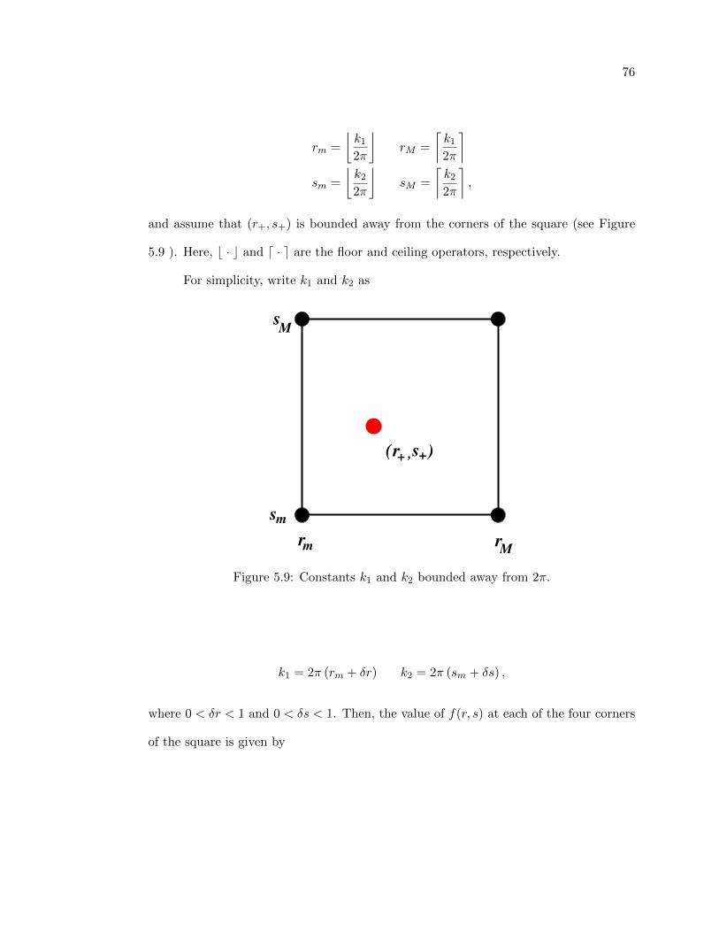
76

rm =

⌊k1

2π

⌋rM =

⌈k1

2π

⌉sm =

⌊k2

2π

⌋sM =

⌈k2

2π

⌉,

and assume that (r+, s+) is bounded away from the corners of the square (see Figure

5.9 ). Here, b · c and d · e are the floor and ceiling operators, respectively.

For simplicity, write k1 and k2 as

,

r r

s

s

m

m

M

M

(r+ s+)

Figure 5.9: Constants k1 and k2 bounded away from 2π.

k1 = 2π (rm + δr) k2 = 2π (sm + δs) ,

where 0 < δr < 1 and 0 < δs < 1. Then, the value of f(r, s) at each of the four corners

of the square is given by

77

f(rm, sm) =4π2δr2 + 4π2δs2

1 + 4π2r2m + 4π2s2

m

blah

f(rM , sm) =4π2 (1− δr)2 + 4π2δs2

1 + 4π2 (rm + 1)2 + 4π2s2m

blah

f(rm, sM ) =4π2δr2 + 4π2 (1− δs)2

1 + 4π2r2m + 4π2 (sm + 1)2

blah

f(rM , sM ) =4π2 (1− δr)2 + 4π2 (1− δs)2

1 + 4π2 (rm + 1)2 + 4π2 (sm + 1)2

From these expressions, it is clear the the size of f (r, s) on the corners of the box depend

on both the size of δr and δs, as well as the size of rm and sm (and, by extension, the

size of k1 and k2). In the case when k1 and k2 are large, the integer pair that minimizes

f (r, s) occurs at the point closest to (r+, s+). However, in the case when k1 and k2

are small, it is possible that the minimizing corner point will not be the one closest to

(r+, s+). In any case, a lower bound for f (r, s) can be established. That is,

ck := minr,s∈Z

f (r, s) = ≥ 4π2 (δr∗)2 + 4π2 (δs∗)2

1 + 4π2[(rm + 1)2 + (sm + 1)2

] , (5.46)

where

δr∗ = min δr, |1− δr|

δs∗ = min δs, |1− δs| .

In the case when k1 and k2 are reasonably small (on the order of 10) and (r+, s+) is

bounded away from the corners of the square, the coercivity constant is reasonably

sized. However, in the case that k1 or k2 is very large, ck may be very small, since

78

the numerator is bounded above by 8π and the denominator can grow without bound.

Thankfully, it is our experience that the constant portions of gauge fields generated

using standard methods tend to be fairly small ( < 15 for all of our test cases).

Case 2: Bk Singular

Let k1 = 2πr0 and k2 = 2πs0 for some integers r0 and s0. In this case, Bk is singular

on VC , and, thus, not coercive. In this case, let UL be the orthogonal complement of

φ0 = ei(k1x+k2y) in VC . That is,

UL =ξ ∈ VC s.t.

⟨ξ, ei(k1x+k2y)

⟩= 0,

or, in terms of Fourier modes,

UL = Span

ei2π(rx+sy) s.t. r, s ∈ Z and r 6= k1

2π, s 6= k2

2π

.

In this case, the integer minimizers are located on the boundary of the larger square in

the rs-plane given by rm ≤ r ≤ rM , sm ≤ s ≤ sM , where

rm =k1

2π− 1, rM =

k1

2π+ 1,

sm =k2

2π− 1, sM =

k2

2π+ 1.

This boundary contains eight potential minimizers of f (r, s) (See Figure 5.10). Again,

the minimizing boundary point varies depending on the relative size of k1 and k2. A

lower bound on ck is given by

ck := minr,s∈Z,(r,s)6=(r+,s+)

f (r, s) = ≥ 4π2

1 + 4π2[(rm + 1)2 + (sm + 1)2

] , (5.47)

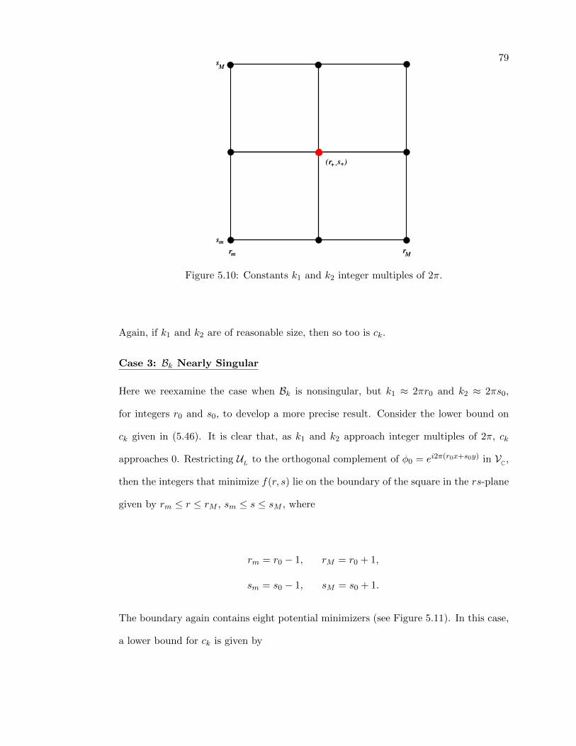
79

m

r+ s+),

Ms

rM

(

r

s

m

Figure 5.10: Constants k1 and k2 integer multiples of 2π.

Again, if k1 and k2 are of reasonable size, then so too is ck.

Case 3: Bk Nearly Singular

Here we reexamine the case when Bk is nonsingular, but k1 ≈ 2πr0 and k2 ≈ 2πs0,

for integers r0 and s0, to develop a more precise result. Consider the lower bound on

ck given in (5.46). It is clear that, as k1 and k2 approach integer multiples of 2π, ck

approaches 0. Restricting UL to the orthogonal complement of φ0 = ei2π(r0x+s0y) in VC ,

then the integers that minimize f(r, s) lie on the boundary of the square in the rs-plane

given by rm ≤ r ≤ rM , sm ≤ s ≤ sM , where

rm = r0 − 1, rM = r0 + 1,

sm = s0 − 1, sM = s0 + 1.

The boundary again contains eight potential minimizers (see Figure 5.11). In this case,

a lower bound for ck is given by

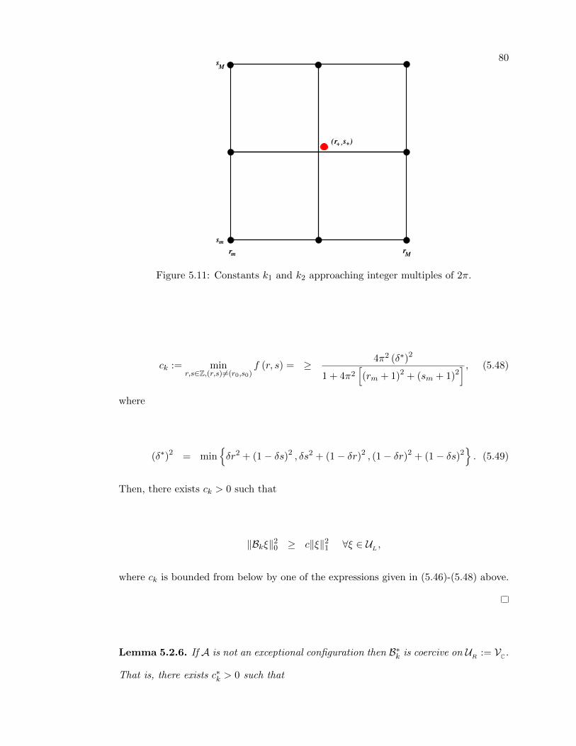
80

m

s

rM

(r+ s+),

M

r

s

m

Figure 5.11: Constants k1 and k2 approaching integer multiples of 2π.

ck := minr,s∈Z,(r,s)6=(r0,s0)

f (r, s) = ≥ 4π2 (δ∗)2

1 + 4π2[(rm + 1)2 + (sm + 1)2

] , (5.48)

where

(δ∗)2 = minδr2 + (1− δs)2 , δs2 + (1− δr)2 , (1− δr)2 + (1− δs)2

. (5.49)

Then, there exists ck > 0 such that

‖Bkξ‖20 ≥ c‖ξ‖21 ∀ξ ∈ UL ,

where ck is bounded from below by one of the expressions given in (5.46)-(5.48) above.

Lemma 5.2.6. If A is not an exceptional configuration then B∗k is coercive on UR := VC.

That is, there exists c∗k > 0 such that

81

‖B∗kξ‖20 ≥ c∗k‖ξ‖21,

for all ξ ∈ UR , where UR := VC. If A is an exceptional configuration then B∗k is coercive

on UR := N (B∗k)⊥. That is, there exists c∗k > 0 such that

‖B∗kξ‖20 ≥ c∗k‖ξ‖21,

for all ξ ∈ UR , where UR := N (B∗k)⊥.

Proof. The proof is very similar to that of Lemma 5.2.5. In fact, the lower bounds on

ck are valid for c∗k as well.

Theorem 5.2.7. If m > 0 or A is not an exceptional configuration then there exist

positive constants cA and CA, which depend on the gauge field, A, such that,

cA‖ψ‖21 ≤ G(ψ,A; 0) ≤ CA‖ψ‖

21,

for all ψ ∈ U , where U := V2C . If m = 0 and A is an exceptional configuration then there

exist positive constants cA and CA, which depend on the gauge field, A, such that,

cA‖ψ‖21 ≤ G(ψ,A; 0) ≤ CA‖ψ‖

21,

for all ψ ∈ U , where U := N (D)⊥.

Proof. The upper-bound is verified first. By repeated use of the triangle and Cauchy’s

inequalities,

82

G(ψ,A; 0) = ‖Dψ‖20

= ‖mψR + (∇x − i∇y)ψL‖20 + ‖mψL + (∇x + i∇y)ψR‖

20

≤ 2(‖mψR‖

20 + ‖∇xψL‖

20 + ‖∇yψL‖

20

+‖mψL‖20 + ‖∇xψR‖

20 + ‖∇yψR‖

20

)= 2

(‖mψR‖

20 + ‖ (∂x −A1)ψL‖

20 + ‖ (∂y −A2)ψL‖

20

+‖mψL‖20 + ‖ (∂x −A1)ψR‖

20 + ‖ (∂y −A2)ψR‖

20

)≤ 2

[‖mψR‖

20 + 2

(‖∂xψL‖

20 + ‖A1ψL‖

20 + ‖∂yψL‖

20 + ‖A2ψL‖

20

)+‖mψL‖

20 + 2

(‖∂xψR‖

20 + ‖A1ψR‖

20 + ‖∂yψR‖

20 + ‖A2ψR‖

20

) ]≤ 2

[‖mψR‖

20 + ‖mψL‖

20 + 2

(‖∂xψR‖

20 + ‖∂yψR‖

20 + ‖∂xψL‖

20 + ‖∂yψL‖

20

)+2(‖A1‖2∞‖ψR‖

20 + ‖A2‖2∞‖ψR‖

20 + ‖A1‖2∞‖ψL‖

20 + ‖A2‖2∞‖ψL‖

20

)]≤

[2m2 + 4

(‖A1‖2∞ + ‖A2‖2∞

)]‖ψ‖20 + 4‖∇ψ‖20

≤ CA‖ψ‖21,

where

CA = max

2m2 + 4(‖A1‖2∞ + ‖A2‖2∞

), 4.

From the proof of Lemma 5.2.5 it is clear that, when verifying the coercivity

condition, care must be taken when the gauge field is an exceptional configuration.

Clearly, if Bk is singular, so too will be the massless Dirac operator, D0. As such, the

cases when Bk is nonsingular and when Bk is singular are handled separately.

Case 1: Bk Nonsingular

Assume that k1 and k2 are bounded comfortably away from integer multiples of 2π.

Then, define U := V2C and UL := UR := VC . From Lemmas 5.2.5 and 5.2.6, there exist

positive constants ck and c∗k such that

83

‖BkψL‖20 ≥ ck‖ψL‖

21 ∀ψL ∈ UL

‖B∗kψR‖20 ≥ c∗k‖ψR‖

21 ∀ψR ∈ UR

Note now that, for any periodic function, z,

UR = e−zUR = VC ,

UL = ezUL = VC .

Thus, from Lemmas 5.2.3 and 5.2.4, there exist positive constants cL and cR such that

‖BψL‖20 ≥ c

L|‖ψL‖21 ∀ψL ∈ UL ,

‖B∗ψR‖20 ≥ cR‖ψR‖

21 ∀ψR ∈ UR .

Then, for all ψ ∈ U ,

‖D0ψ‖20 =

∥∥∥∥∥∥∥ 0 B

−B∗ 0

ψR

ψL

∥∥∥∥∥∥∥

2

0

= ‖BψL‖20 + ‖B∗ψR‖

20

≥ cL‖ψL‖21 + cR‖ψR‖

21

≥ c0‖ψ‖21,

where

c0 = min cR , cL .

Finally, from the coercivity of D0 on U and Lemma 5.2.2, there exists some positive

constant cA such that

84

‖Dψ‖20 ≥ cA‖ψ‖21,

where

cA = minck[(‖e−z‖2∞

)max

‖ez‖2∞ + 2‖∇ez‖2∞, 2‖ez‖2∞

]−1,

c∗k[(‖ez‖2∞

)max

‖e−z‖2∞ + 2‖∇e−z‖2∞, 2‖e−z‖2∞

]−1,

and ck and c∗k are both bounded from below by (5.46).

Case 2: Bk Singular

In the case that the gauge field is an exceptional configuration, the problem is formulated

in the orthogonal complement of φ0 = ei(k1x+k2y). Define both UL and UR according to

UL = UR :=ξ ∈ VC s.t.

⟨ξ, ei(k1x+k2y)

⟩= 0.

Again, from Lemmas 5.2.5 and 5.2.6, there exist positive constants cL and cR such that

‖BkψL‖20 ≥ c

L|‖ψL‖21 ∀ψL ∈ UL

‖B∗kψR‖20 ≥ cR‖ψR‖

21 ∀ψR ∈ UR .

Define UL and UR according to

UL :=ξ ∈ VC s.t.

⟨ξ, ez+i(k1x+k2y)

⟩= 0

UR :=ξ ∈ VC s.t.

⟨ξ, e−z+i(k1x+k2y)

⟩= 0.

Then, from Lemmas 5.2.3 and 5.2.4, there exist positive constants cL and cR such that

85

‖BψL‖20 ≥ c

L|‖ψL‖21 ∀ψL ∈ UL ,

‖B∗ψR‖20 ≥ cR‖ψR‖

21 ∀ψR ∈ UR .

Finally, define U by

U = UR ⊗ UL .

The remainder of the proof is identical to that in Case 1.

Case 3: Bk Nearly Singular

In the case that the gauge field is near an exceptional configuration, that is, k1 ≈ 2πr0

and k2 ≈ 2πs0 for some integers r0 and s0, the problem is formulated in the orthogonal

complement of φ0 = ei2π(r0x+s0y). Define both UL and UR according to

UL = UR :=ξ ∈ VC s.t.

⟨ξ, ei2π(r0x+s0y)

⟩= 0.

Then, the remainder of the proof case is identical to Case 2.

5.2.2 Implications

H1-ellipticity of the least-squares functional has two implications for the least-

squares solution process. First, because the functional is H1-elliptic, it can be shown

that an optimal O (N) multilevel iterative method exists that can solve the resulting

linear system [54].

Second, it suggests an alternate argument that the discrete least-squares operator,

DLS , does not suffer from species doubling. The application of the least-squares operator

involves multiplication by matrix L. The absence of species doubling requires that this

86

application does not map oscillatory modes onto smooth modes. Recall that, from the

coercivity condition on the least-squares functional,

‖Dψ‖20 ≥ cA‖ψ‖21

= cA(‖ψ‖20 + ‖∇ψ‖20

)≥ cA‖∇ψ‖

20.

Thus,

‖Dψ‖20‖∇ψ‖20

≥ cA ∀ψ ∈ V2C . (5.50)

Recall, from (5.32), that

‖Dψh‖20 =⟨Lψ,ψ

⟩l2. (5.51)

Similarly,

‖∇ψh‖20 =⟨Aψ,ψ

⟩l2. (5.52)

where A is the standard Galerkin discretization of the constant coefficient Laplacian.

Then, combining (5.50) - (5.52) yields a discrete coercivity condition

⟨Lψ,ψ

⟩⟨Aψ,ψ

⟩ ≥ cA ∀ψ ∈ N2C . (5.53)

Clearly, the discrete Laplacian, A, maps oscillatory modes to the high end of the spec-

trum. The coercivity bound, (5.53), implies that L must map oscillatory modes to the

high end of the spectrum as well. Thus, the application of L cannot result in species

doubling.

87

5.3 Numerical Experiments

In this section, the use of classical algebraic multigrid (AMG) is investigated as

a preconditioner for the solution of the linear system appearing in Step 3 of Algorithm

5.3. That is,

Lζ = Kg. (5.54)

The conjugate gradient (CG) algorithm is used to accelerate the solution process [33],

[47]. Later, we compare the use of AMG preconditioned CG applied to (5.54) to adaptive

smoothed aggregation (αSA) preconditioned CG, when applied to the Dirac-Wilson

operator. A brief introductions to general multigrid theory is given. This is then

extended to AMG and αSA.

5.3.1 Multigrid Methods

Multigrid methods are a large class of iterative methods used to solve linear

systems of equations of the form

Ax = b. (5.55)

Let x be the true solution of (5.55) and y be some approximations to x. Two quantities

of interest are the residual and error of the approximation, given by

r = b−Ay,

e = x− y,

respectively. Some simple algebra provides a relationship between the error and the

residual. This relationship, called the residual-error equation, is given by

88

Ae = r.

Naturally, if the error of the current iterate was known exactly, then the true solution

is obtained by correcting the current iterate according to

x = y + e.

The error is generally not known in practice. However, if an approximation to the

current error is available, call it e, it can be used to correct the current iterate. An

iteration based on this correction would set

y ← y + e,

at each step in the iteration. In multigrid methods, a sequence of coarse grids are used

to compute an approximation to the current error in an inexpensive manner.

At the heart of all multigrid methods are two complementary processes: relaxation

and coarse-grid correction. Relaxation is a local process that effectively reduces some

portion of the error in the current iterate. Error that is not effectively reduced by

relaxation is called algebraically smooth. A general step in a relaxation method sets

y ← y +M−1r, (5.56)

where M is some approximation of the matrix A. The relaxation step can also be

formulated in terms of its action on the error of the current approximation. That is, in

a single step of relaxation, the error is updated according to

e ← e−M−1Ae. (5.57)

89

This provides a useful characterization of algebraically smooth error. Suppose the error

is such that

M−1Ae ≈ 0,

relative to e. Then, the relaxation step given in (5.57) fails to reduce a significant

portion of the error. Thus, algebraically smooth error is often said to be near-kernel.

Coarse-grid correction is a global process that uses a coarse grid to obtain an

approximation to algebraically smooth error. This approximation of the error is then

used to correct the current approximation. Suppose that the original grid, or the fine

grid, has N points. Now, suppose some coarse grid exists with Nc points, where Nc <<

N . Let P ∈ CN×Nc be the so called interpolation operator, that maps objects from

the coarse grid to the fine grid. The so called restriction operator maps objects on the

fine grid to the coarse grid. There are many choices for the restriction operator. For

the methods in this thesis, we take P t to be the restriction operator, where P is the

previously introduced interpolation operator. Now, suppose that some approximation

to the fine-grid error is computed on the coarse grid; call it ec. Then, a correction to

the fine-grid approximation can be made by setting

y ← y + Pec.

Note that the error in this iteration is updated according to

e ← e− Pec. (5.58)

The coarse-grid error is obtained by solving a coarse-grid version of the residual-error

equation:

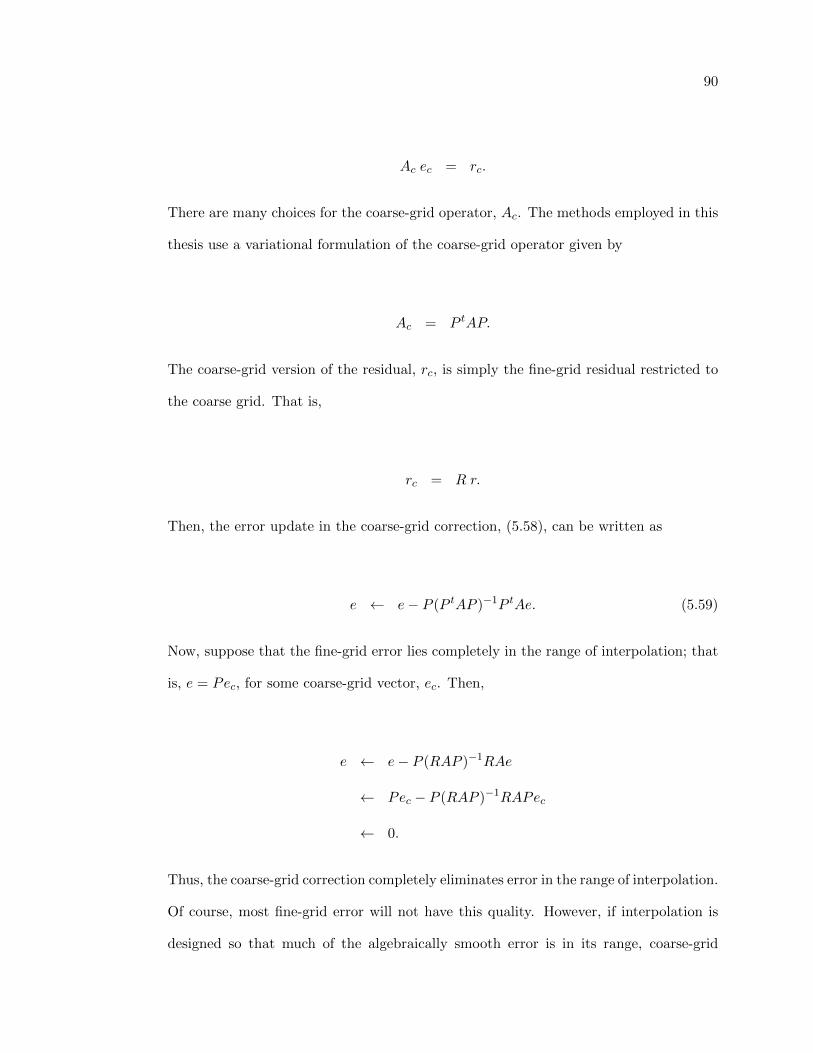
90

Ac ec = rc.

There are many choices for the coarse-grid operator, Ac. The methods employed in this

thesis use a variational formulation of the coarse-grid operator given by

Ac = P tAP.

The coarse-grid version of the residual, rc, is simply the fine-grid residual restricted to

the coarse grid. That is,

rc = R r.

Then, the error update in the coarse-grid correction, (5.58), can be written as

e ← e− P (P tAP )−1P tAe. (5.59)

Now, suppose that the fine-grid error lies completely in the range of interpolation; that

is, e = Pec, for some coarse-grid vector, ec. Then,

e ← e− P (RAP )−1RAe

← Pec − P (RAP )−1RAPec

← 0.

Thus, the coarse-grid correction completely eliminates error in the range of interpolation.

Of course, most fine-grid error will not have this quality. However, if interpolation is

designed so that much of the algebraically smooth error is in its range, coarse-grid

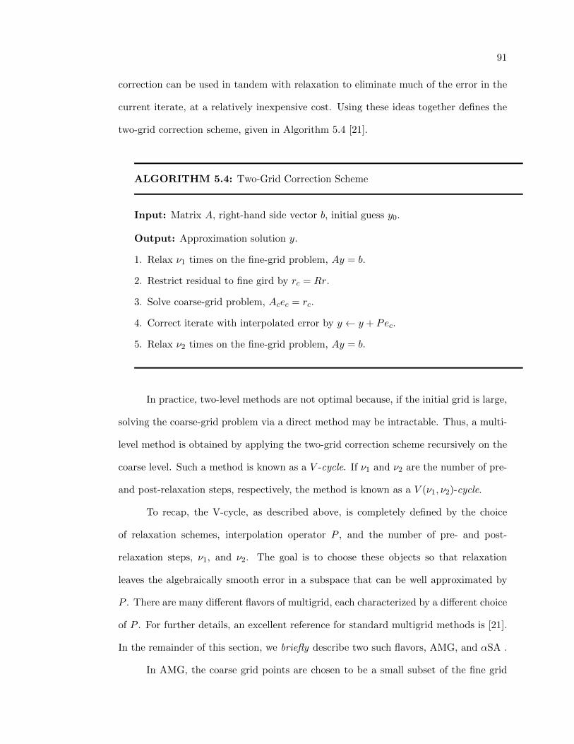
91

correction can be used in tandem with relaxation to eliminate much of the error in the

current iterate, at a relatively inexpensive cost. Using these ideas together defines the

two-grid correction scheme, given in Algorithm 5.4 [21].

ALGORITHM 5.4: Two-Grid Correction Scheme

Input: Matrix A, right-hand side vector b, initial guess y0.

Output: Approximation solution y.

1. Relax ν1 times on the fine-grid problem, Ay = b.

2. Restrict residual to fine gird by rc = Rr.

3. Solve coarse-grid problem, Acec = rc.

4. Correct iterate with interpolated error by y ← y + Pec.

5. Relax ν2 times on the fine-grid problem, Ay = b.

In practice, two-level methods are not optimal because, if the initial grid is large,

solving the coarse-grid problem via a direct method may be intractable. Thus, a multi-

level method is obtained by applying the two-grid correction scheme recursively on the

coarse level. Such a method is known as a V -cycle. If ν1 and ν2 are the number of pre-

and post-relaxation steps, respectively, the method is known as a V (ν1, ν2)-cycle.

To recap, the V-cycle, as described above, is completely defined by the choice

of relaxation schemes, interpolation operator P , and the number of pre- and post-

relaxation steps, ν1, and ν2. The goal is to choose these objects so that relaxation

leaves the algebraically smooth error in a subspace that can be well approximated by

P . There are many different flavors of multigrid, each characterized by a different choice

of P . For further details, an excellent reference for standard multigrid methods is [21].

In the remainder of this section, we briefly describe two such flavors, AMG, and αSA .

In AMG, the coarse grid points are chosen to be a small subset of the fine grid

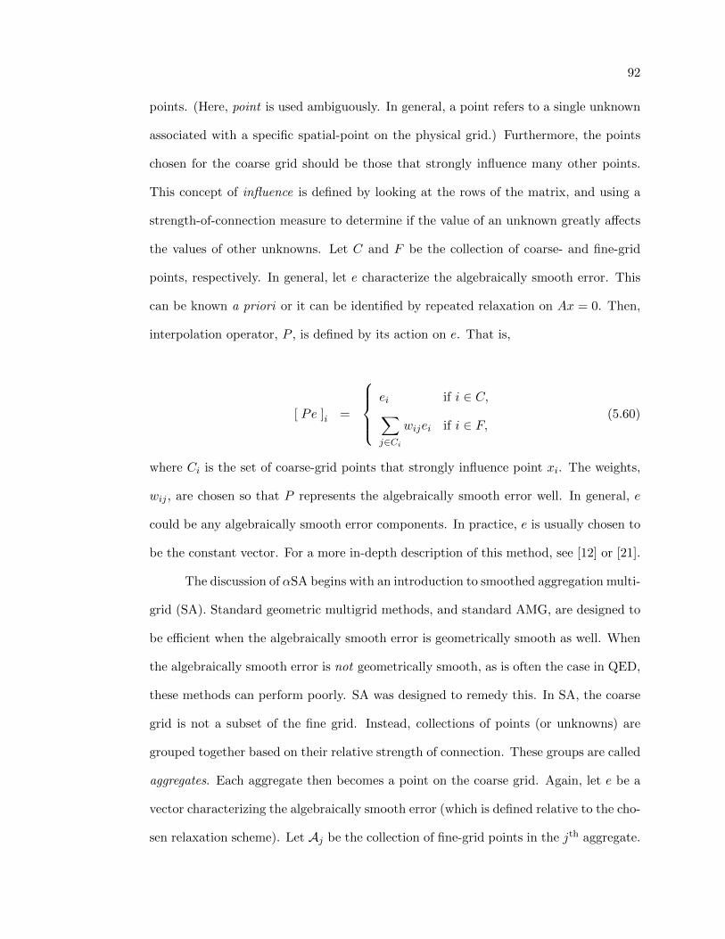
92

points. (Here, point is used ambiguously. In general, a point refers to a single unknown

associated with a specific spatial-point on the physical grid.) Furthermore, the points

chosen for the coarse grid should be those that strongly influence many other points.

This concept of influence is defined by looking at the rows of the matrix, and using a

strength-of-connection measure to determine if the value of an unknown greatly affects

the values of other unknowns. Let C and F be the collection of coarse- and fine-grid

points, respectively. In general, let e characterize the algebraically smooth error. This

can be known a priori or it can be identified by repeated relaxation on Ax = 0. Then,

interpolation operator, P , is defined by its action on e. That is,

[ Pe ]i =

ei if i ∈ C,∑j∈Ci

wijei if i ∈ F,(5.60)

where Ci is the set of coarse-grid points that strongly influence point xi. The weights,

wij , are chosen so that P represents the algebraically smooth error well. In general, e

could be any algebraically smooth error components. In practice, e is usually chosen to

be the constant vector. For a more in-depth description of this method, see [12] or [21].

The discussion of αSA begins with an introduction to smoothed aggregation multi-

grid (SA). Standard geometric multigrid methods, and standard AMG, are designed to

be efficient when the algebraically smooth error is geometrically smooth as well. When

the algebraically smooth error is not geometrically smooth, as is often the case in QED,

these methods can perform poorly. SA was designed to remedy this. In SA, the coarse

grid is not a subset of the fine grid. Instead, collections of points (or unknowns) are

grouped together based on their relative strength of connection. These groups are called

aggregates. Each aggregate then becomes a point on the coarse grid. Again, let e be a

vector characterizing the algebraically smooth error (which is defined relative to the cho-

sen relaxation scheme). Let Aj be the collection of fine-grid points in the jth aggregate.

93

Then interpolation operator P is defined according to

[ P ]ij =

ei if i ∈ Aj ,

0 otherwise.

(5.61)

Note that, with P defined in this manner, error vector e is exactly in the range of inter-

polation. Thus, a coarse-grid correction completely eliminates e. Often, this choice of P

leads to an effective multigrid method. More often, though, e is only a characterization

of some of the algebraically smooth error. If the remainder of the error is not captured

well by P , then convergence of the method will be poor. To remedy this, the columns of

P are smoothed by applying one step of relaxation to homogeneous equation with each

column of P as the initial guess. (Note that the relaxation scheme used to smooth P

is often different than the one used in the V-cycle. Usually weighted-Jacobi is chosen.)

This smoothing allows P to capture algebraically smooth error vector e, as well as other

error that is locally similar to e. Thus, smoothing enriches the space of vectors that can

be well represented by P .

We have said nothing about how to obtain e. In many problems, such as linear

elasticity, the algebraically smooth error modes are known a priori. In the case that

they are not known, they can be obtained by relaxing on Ax = 0. This adaptive

exposure of the algebraically smooth error is the basis for αSA. In the setup phase,

relaxation is applied to the homogeneous problem until convergence stalls. Then, the

resulting smooth error component is used to form P . Note that it is possible that the

algebraically smooth error is spanned by more than one distinct smooth error vector.

In this case, a V-cycle would effectively reduce error similar to the vector used to build

P , while leaving the remaining error largely untouched; P can then be constructed to

accurately interpolate more than one error component. Note that if P is built to handle

two distinct error components, then P will have twice as many columns. This leads to

94

a coarse-grid operator that is twice as large.

To build an interpolation operator to handle more than one prototype error com-

ponent, we first relax on Ax = 0 until convergence stalls. P is then constructed based

on this component and used to define a V-cycle. Then, we iterate on Ax = 0 with

the V-cycle. When this stalls, the resulting prototype error vector will be algebraically

smooth with respect to the current method, instead of relaxation. P is then extended to

accurately capture the new error component as well. This continues until convergence

of the current method, applied to the homogeneous system of equations, is satisfactory.

The setup phase is then exited and the resulting V-cycle is used to solve the target (in-

homogeneous) problem. Note that this process leads to a much higher setup cost than

that of AMG, where only the coarse-fine partitioning of the grid and the computation of

the interpolation weights are needed. For a more in-depth description of SA and αSA,

see [18] or [49].

Finally, we introduce some terminology that allows us to compare the compu-

tational cost of these multilevel methods. Let operator complexity, σ, be the ratio of

total number of nonzeros in the operators on all grids in the multigrid hierarchy to the

number of nonzeros in the fine-grid operator alone. Then σ gives an indication of how

much work is required to preform a computation, such as one residual calculation, on all

grid levels compared to performing that computation on just the fine grid [21]. Since a

multigrid V(ν1, ν2)-cycle performs (ν1 + ν2) relaxation steps on each grid level, and one

residual calculation on each grid level, the operator complexity allows us to estimate

the total cost of such a cycle relative to the cost of one relaxation step on the fine grid.

Let one work unit (WU) be the cost of doing one matrix-vector multiply on the fine

grid. Then, the cost of a single V(ν1, ν2)-cycle is approximately σ(ν1 + ν2 + 1) WUs.

Finally, define η to be the number of work units needed to improve the current iterate

by one digit of accuracy. Then

95

η = σ (ν1 + ν2 + 1)log .1

log ρ, (5.62)

where ρ is the convergence factor observed in the method [20].

5.3.2 Numerical Results

Linear system (5.54) clearly contains complex entries. To avoid working in com-

plex arithmetic, the following equivalent real formulation (ERF) of (5.54) is solved

instead:

X −Y

Y X

x

y

=

a

b

, (5.63)

where X,Y are real-valued matrices satisfying L = X+ iY, ζ = x+ iy, and Kg = a+ ib.

Note that Y is skew-Hermitian so that (5.63) is a symmetric real system. Moreover,

since the complex matrix is Hermitian positive semidefinite, the real system is symmetric

positive semidefinite. In particular, we are interested in how the performance of AMG

preconditioned CG (AMG-PCG) and αSA preconditioned CG (αSA-PCG) varies with

fermion mass, m, gauge field temperature parameter, β, and lattice size, N .

In the following tests, AMG-PCG and αSA-PCG are applied to (5.63). For AMG-

PCG, a single V(1,1)-cycle with Gauss-Seidel relaxation is used as the preconditioner

in each step of CG. For αSA-PCG, a single V(2,2)-cycle used as the preconditioner is

constructed using 2 prototype error components to build the interpolation operator.

The relaxation method used is Gauss-Seidel. Aggregation is done algebraically. Each

method is applied to (5.63) with a zero right-hand side and random initial guess. The

iteration is terminated when the relative residual in the iteration has been decreased by

a factor of 10−6. Average convergence factors are computed by applying the method to

operators constructed using 20 distinct gauge fields.

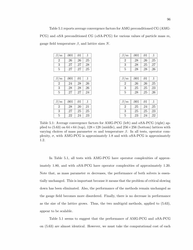
96

Table 5.1 reports average convergence factors for AMG preconditioned CG (AMG-

PCG) and αSA preconditioned CG (αSA-PCG) for various values of particle mass m,

gauge field temperature β, and lattice sizes N .

β/m .001 .01 .1

2 .26 .26 .25

3 .27 .27 .28

5 .27 .27 .25

β/m .001 .01 .1

2 .24 .28 .26

3 .28 .28 .26

5 .27 .27 .24

β/m .001 .01 .1

2 .28 .20 .21

3 .27 .25 .25

5 .22 .24 .23

β/m .001 .01 .1

2 .28 .26 .25

3 .28 .25 .27

5 .28 .28 .26

β/m .001 .01 .1

2 .26 .26 .25

3 .25 .25 .23

5 .28 .25 .26

β/m .001 .01 .1

2 .25 .24 .25

3 .25 .25 .23

5 .23 .24 .22

Table 5.1: Average convergence factors for AMG-PCG (left) and αSA-PCG (right) ap-plied to (5.63) on 64×64 (top), 128×128 (middle), and 256×256 (bottom) lattices withvarying choices of mass parameter m and temperature β. In all tests, operator com-plexity, σ, with AMG-PCG is approximately 1.8 and with αSA-PCG is approximately1.2.

In Table 5.1, all tests with AMG-PCG have operator complexities of approx-

imately 1.80, and with αSA-PCG have operator complexities of approximately 1.20.

Note that, as mass parameter m decreases, the performance of both solvers is essen-

tially unchanged. This is important because it means that the problem of critical slowing

down has been eliminated. Also, the performance of the methods remain unchanged as

the gauge field becomes more disordered. Finally, there is no decrease in performance

as the size of the lattice grows. Thus, the two multigrid methods, applied to (5.63),

appear to be scalable.

Table 5.1 seems to suggest that the performance of AMG-PCG and αSA-PCG

on (5.63) are almost identical. However, we must take the computational cost of each

97

type of V-cycle used in the two methods into consideration. Recall that the AMG

V(1,1)-cycle uses two fewer relaxation steps on each level than the V(2,2)-cycle used in

αSA. On the other hand, the smaller operator complexity associated with αSA means

that the relaxation and residual computations done in αSA are cheaper than those done

in AMG. To accurately compare the performance of the two methods we look at the

computational cost required by each to reduce the error in the current iteration by one

digit of accuracy. Table 5.2 reports average η-values for each method applied to (5.63)

on a 64× 64 lattice, where η is defined in (5.62).

β/m .001 .01 .1

2 9.2 9.2 9.0

3 9.5 9.5 9.8

5 9.5 9.5 9.0

β/m .001 .01 .1

2 10.9 10.3 10.0

3 10.9 10.0 10.5

5 10.9 10.9 10.3

Table 5.2: Average η-values for AMG-PCG (left) and αSA-PCG (right) applied to (5.63)on a 64× 64 lattice with varying choices of mass parameter m and temperature β.

From Table 5.2 we see that in overall accuracy per computational cost, AMG-PCG

performs roughly 10% better than αSA-PCG. Furthermore, these comparisons do not

take into consideration the setup cost of the two methods. Because αSA requires the

computation of prototype error components the setup cost for αSA is inherently more

expensive than for AMG. Although this is minimized in the present case because only

2 prototype error components are used, the αSA setup phase is still considerably more

expensive than that of AMG.

It is interesting to compare the performance of an algebraic multigrid method

on the discrete least-squares operator, DLS , and the traditional Dirac-Wilson operator,

DW , given by (3.26). Since AMG-PCG performed better in our tests than αSA-PCG

we will use it here. Unfortunately, AMG-PCG is not an effective solver for the Dirac-

Wilson operator because of its rich near-kernel space [13]. Instead, αSA-PCG is used.

The non-Hermiticity of DW makes the problem difficult to solve with standard αSA

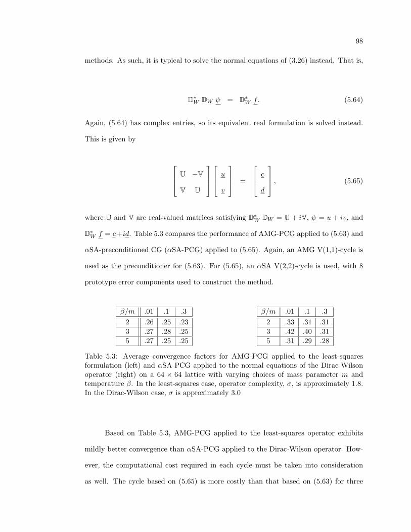
98

methods. As such, it is typical to solve the normal equations of (3.26) instead. That is,

D∗W DW ψ = D∗W f. (5.64)

Again, (5.64) has complex entries, so its equivalent real formulation is solved instead.

This is given by

U −V

V U

u

v

=

c

d

, (5.65)

where U and V are real-valued matrices satisfying D∗W DW = U + iV, ψ = u + iv, and

D∗W f = c+id. Table 5.3 compares the performance of AMG-PCG applied to (5.63) and

αSA-preconditioned CG (αSA-PCG) applied to (5.65). Again, an AMG V(1,1)-cycle is

used as the preconditioner for (5.63). For (5.65), an αSA V(2,2)-cycle is used, with 8

prototype error components used to construct the method.

β/m .01 .1 .3

2 .26 .25 .23

3 .27 .28 .25

5 .27 .25 .25

β/m .01 .1 .3

2 .33 .31 .31

3 .42 .40 .31

5 .31 .29 .28

Table 5.3: Average convergence factors for AMG-PCG applied to the least-squaresformulation (left) and αSA-PCG applied to the normal equations of the Dirac-Wilsonoperator (right) on a 64 × 64 lattice with varying choices of mass parameter m andtemperature β. In the least-squares case, operator complexity, σ, is approximately 1.8.In the Dirac-Wilson case, σ is approximately 3.0

Based on Table 5.3, AMG-PCG applied to the least-squares operator exhibits

mildly better convergence than αSA-PCG applied to the Dirac-Wilson operator. How-

ever, the computational cost required in each cycle must be taken into consideration

as well. The cycle based on (5.65) is more costly than that based on (5.63) for three

99

reasons. First, the operator in (5.65) has approximately 88% more nonzeros than that

in (5.63). Thus, one work unit with respect to (5.65) involves approximately 1.88 times

as much computation as a work unit with respect to (5.63). Second, the V(2,2)-cycle

used for αSA-PCG requires 2 more relaxations on each level than the V(1,1)-cycle used

for AMG. Finally, the reported operator complexity of the cycle for (5.65) is approxi-

mately 3.0, versus 1.8 for (5.63). To directly compare the efficiency of the two methods,

η-values are computed for each, cost in terms of a work unit with respect to (5.63). For

clarity, define ηLS and ηW by

ηLS = σLS (ν1 + ν2 + 1)log .1

log ρLS, (5.66)

ηW = 1.88× σW (ν1 + ν2 + 1)log .1

log ρW, (5.67)

where σLS and ρLS are the operator complexity and convergence factor of the method

applied to (5.63), respectively, and σW and ρW are the operator complexity and con-

vergence factor of the method applied to (5.65), respectively. Then, ηW specifies the

number of work units with respect to the least-squares operator that are needed to

improve the accuracy of the current iterate by one digit.

Table 5.4 gives the previously define η-values for the results provided in Table

5.3. Furthermore, the ratio ηW /ηLS gives an estimate of the speedup obtained in using

the least-squares discretization over the Dirac-Wilson discretization. These ratios are

given in Table 5.5.

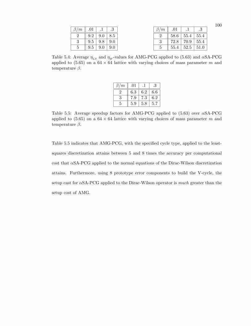
100β/m .01 .1 .3

2 9.2 9.0 8.5

3 9.5 9.8 9.0

5 9.5 9.0 9.0

β/m .01 .1 .3

2 58.6 55.4 55.4

3 72.8 70.9 55.4

5 55.4 52.5 51.0

Table 5.4: Average ηLS and ηW -values for AMG-PCG applied to (5.63) and αSA-PCGapplied to (5.65) on a 64 × 64 lattice with varying choices of mass parameter m andtemperature β.

β/m .01 .1 .3

2 6.3 6.2 6.6

3 7.9 7.3 6.2

5 5.9 5.8 5.7

Table 5.5: Average speedup factors for AMG-PCG applied to (5.63) over αSA-PCGapplied to (5.65) on a 64 × 64 lattice with varying choices of mass parameter m andtemperature β.

Table 5.5 indicates that AMG-PCG, with the specified cycle type, applied to the least-

squares discretization attains between 5 and 8 times the accuracy per computational

cost that αSA-PCG applied to the normal equations of the Dirac-Wilson discretization

attains. Furthermore, using 8 prototype error components to build the V-cycle, the

setup cast for αSA-PCG applied to the Dirac-Wilson operator is much greater than the

setup cost of AMG.

Chapter 6

Least-Squares Finite Elements for a Transformed Schwinger Model

In this chapter a discrete approximation to the 2D Schwinger model is formulated

by applying the least-squares methodology to the transformed system described in Sec-

tion 2.2.3. Again, naively applying least-squares directly to the governing equations

results in an algorithm that is not gauge covariant. To remedy this, the same gauge fix-

ing concept used in Chapter 5 is applied. It is demonstrated that the resulting discrete

solution process satisfies gauge covariance and chiral symmetry, and does not suffer

from species doubling. Next, the least-squares functional for the transformed system is

shown to be H1-elliptic. Finally, numerical experiments are carried out, using adaptive

smoothed aggregation multigrid, as well as classic algebraic multigrid, as precondition-

ers for solving the resulting linear system. The results show that the discretization of

the transformed system can be solved very efficiently by algebraic multigrid methods.

6.1 Discretization of the Transformed System

Again, the first objective is to discretize the 2D Schwinger model, given by

mI B

−B∗ mI

ψR

ψL

=

fR

fL

, (6.1)

where B (A) = ∇x − i∇y = (∂x − iA1) − i (∂y − iA2). Recall that, if the gauge field

has the usual Helmholtz decomposition, A = ∇⊥u+∇v + k, then B and B∗ transform

102

according to

B (A) ez = ezBk, (6.2)

B∗ (A) e−z = e−zB∗k, (6.3)

where z = u + iv and Bk = (∂x − ik1) − i (∂y − ik2). Define a transformation, Q,

according to

Q =

e−zI 0

0 ezI

. (6.4)

Setting ψ = Qξ in (6.1) yields

me−zI ezBk

−e−zB∗k mezI

ξR

ξL

=

fR

fL

. (6.5)

Denote this transformed operator in (6.5) by D (A). Note that D still depends on

gauge field A because the gauge data is contained in the exponential terms. Then, if

an efficient method of discretizing and solving the transformed system (6.5) exists, the

original system, (6.1), can be solved by first solving (6.5) and then setting ψ = Qξ.

Thus, a solution process for the continuum problem, based on this transformation, is

given in Algorithm 6.1.

Note that care must be taken with the boundary conditions prescribed to the

auxiliary function ξ. Requiring ψ to be periodic on R is, of course, equivalent to

requiring Qξ to be periodic on R. But, since z ∈ WR is periodic by definition, Qξ will

be periodic as long as ξ is. Thus, in Algorithm 6.1, the periodicity of ξ alone is enforced.

The auxiliary continuum equation in Step 1 of Algorithm 6.1 is discretized using

least-squares finite elements by formulating the solution of (6.5) as a minimization

problem:

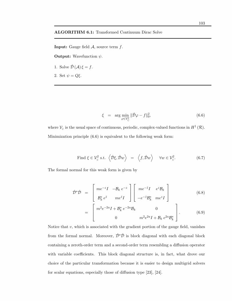
103

ALGORITHM 6.1: Transformed Continuum Dirac Solve

Input: Gauge field A, source term f .

Output: Wavefunction ψ.

1. Solve D (A) ξ = f .

2. Set ψ = Qξ.

ξ = arg minϕ∈V2

C

‖Dϕ− f‖20, (6.6)

where VC is the usual space of continuous, periodic, complex-valued functions in H1 (R).

Minimization principle (6.6) is equivalent to the following weak form:

Find ξ ∈ V2C s.t.

⟨Dξ, Dw

⟩=

⟨f, Dw

⟩∀w ∈ V2

C . (6.7)

The formal normal for this weak form is given by

D∗D =

me−zI −Bk e−z

B∗k ez mezI

me−zI ezBk

−e−zB∗k mezI

(6.8)

=

m2e−2uI + B∗k e−2uBk 0

0 m2e2uI + Bk e2uB∗k

. (6.9)

Notice that v, which is associated with the gradient portion of the gauge field, vanishes

from the formal normal. Moreover, D∗D is block diagonal with each diagonal block

containing a zeroth-order term and a second-order term resembling a diffusion operator

with variable coefficients. This block diagonal structure is, in fact, what drove our

choice of the particular transformation because it is easier to design multigrid solvers

for scalar equations, especially those of diffusion type [23], [24].

104

The least-squares solution is obtained by restricting the minimization problem in

(6.6) and, thus, the weak form in (6.7), to the usual finite-dimensional space, VhC ⊂ VC .

That is, the solution must satisfy the following weak form:

Find ξh ∈(VhC)2

s.t.⟨Dξh, Dwh

⟩=

⟨fh, Dwh

⟩∀wh ∈

(VhC)2. (6.10)

Step 2 of Algorithm 6.1 obtains the solution by setting ψ = Qξ, which can be formulated

as a weak form as well:

Find ψh ∈(VhC)2

s.t.⟨ψh, wh

⟩=

⟨Qξh, wh

⟩∀wh ∈

(VhC)2. (6.11)

Note that this is just the L2-projection of Qξh onto(VhC)2

. These processes define the

following potential algorithm for the solution of (6.1).

ALGORITHM 6.2: Transformed Least-Squares Dirac Solve

Input: Gauge field A, source term f .

Output: Wavefunction ψ.

1. Compute u and v such that A = Cu+ Gv + k.

2. Map u 7→ uh and v 7→ vh.

3. Map f 7→ fh ∈(VhC)2

.

4. Find ξh ∈(VhC)2

s.t.⟨Dξh, Dwh

⟩=⟨fh, Dwh

⟩∀wh ∈

(VhC)2

,

5. Find ψh ∈(VhC)2

s.t.⟨ψh, wh

⟩=⟨Qξh, wh

⟩∀wh ∈

(VhC)2

.

6. Map ψh 7→ ψ ∈ (NC)2.

105

6.1.1 Gauge Covariance

Unfortunately, Algorithm 6.2, as it stands, does not satisfy the principle of gauge

covariance. The same difficulty discovered in the development of the algorithm in Chap-

ter 5 is present here. That is, gauge covariance is thwarted because the proper rela-

tionship between f and T∗ω f is lost when these vectors are projected into the finite

element space. The transformed algorithm suffers a similar problem in the weak form

that relates the auxiliary solution, ξh, and the solution to the original problem, ψh,

appearing in Step 5 of Algorithm 6.2. Fortunately, both problems are remedied using

the same gauge fixing idea employed in Chapter 5.

As before, gauge covariance is retained by transforming the input data into an

equivalent set corresponding to a divergence free gauge field. That is, given discrete

source term, f , and gauge data,

A = A0 + Gv,

an auxiliary problem is solved based on

A = A0

and

f = T∗v f.

The solution is then obtained by setting

ψ = Tv ψ,

106

where ψ is the solution based on the transformed data. Note the implication of this for

the transformed system. Since the gauge field does not contain a gradient, transforma-

tion Q only involves the smoother curl portion of the gauge field. That is,

Q = Q(u) =

e−uI 0

0 euI

. (6.12)

A gauge covariant algorithm based on the transformed system is formulated in

Algorithm 6.3.

ALGORITHM 6.3: Transformed Gauge Covariant Least-Squares Dirac Solve

Input: Gauge field A, source term f .

Output: Wavefunction ψ.

1. Compute u and v such that A = Cu+ Gv + k.

2. Set g = T∗v f

3. Map u 7→ uh.

4. Map g 7→ gh ∈(VhC)2

.

5. Find ξh ∈(VhC)2

s.t.⟨Dξh, Dwh

⟩=⟨fh, Dwh

⟩∀wh ∈

(VhC)2

,

where D = D(∇⊥uh + k)

6. Find ζh ∈(VhC)2

s.t.⟨ζh, wh

⟩=⟨Qξh, wh

⟩∀wh ∈

(VhC)2

,

where Q = Q(uh)

7. Map ζh 7→ ζ ∈ (NC)2.

8. Set ψ = Tv ζ

To avoid serious complication of notation, the same symbols used to represent

discrete operators in Chapter 5 (L, K and DLS) are used again here. However, their

use in this chapter is entirely self contained, so there should be no confusion. Using the

107

nodal basis for VhC , the following matrix equation for Step 5 of Algorithm 6.3 can be

established:

Lξ = Kg, (6.13)

where ξ and g are the coefficients in the expansions of ξh and gh, respectively. Note that,

since the discrete values of ξ and g naturally coincide with the expansion coefficients

of ξh and gh, respectively, it is convenient to represent them using the same notation.

Matrices L and K are given according to

L :=

L11 0

0 L22

, (6.14)

L11 := m2M− + L−xx + L−yy + i(L−xy − L−yx), (6.15)

L22 := m2M+ + L+xx + L+

yy + i(L+xy − L+

yx), (6.16)

K =

mM+ B+x − iB+

y

B−x + iB−y mM−

, (6.17)

where

108

[ L±xx ]j,k = < e±u(∂x − ik1)φk, e±u(∂x − ik1)φj >,

[ L±xy ]j,k = < e±u(∂x − ik1)φk, e±u(∂y − ik2)φj >,

[ L±yx ]j,k = < e±u(∂y − ik2)φk, e±u(∂x − ik1)φj >,

[ L±yy ]j,k = < e±u(∂y − ik2)φk, e±u(∂y − ik2)φj >,

[ B±x ]j,k = < φk, e±u(∂y − ik2)φj >,

[ B±y ]j,k = < φk, e±u(∂x − ik1)φj >,

[ M± ]j,k = < e±uφk, e±uφj > .

Here, φj is the usual bilinear finite element basis function associated with the jth lattice

site. Similarly, a linear system can be developed to replace the weak form in Step 6 of

Algorithm 6.3:

Pζ = Qξ. (6.18)

where

P =

P0 0

0 P0

, Q =

Q− 0

0 Q+

, (6.19)

and

[ P0 ]j,k =< φk, φj >, [ Q± ]j,k =< e±uφk, φj > . (6.20)

Using arguments similar to those employed in Chapter 5, it is easy to see that L

and K are singular only when m = 0 and Ah0 is an exceptional configuration. Further-

more, matrices P and Q are nonsingular for all masses and gauge configurations.

109

Using the above matrix representations, Algorithm 6.3 can be formulated com-

pletely in the discrete setting. This is summarized in Algorithm 6.4.

ALGORITHM 6.4: Discrete Transformed Gauge Covariant Least-SquaresDirac Solve

Input: Gauge field A, source term f .

Output: Wavefunction ψ.

1. Compute u and v such that A = Cu+ Gv + k.

2. Set g = T∗v f

3. Compute ξ = L−1Kg

4. Compute ζ = P−1Qξ

5. Set ψ = Tv ζ

Combining Steps 2-5 in Algorithm 6.4 yields an expression for the discrete least-squares

propagator, hereafter denoted by D−1LS :

D−1LS = Tv P−1Q L−1K T∗v. (6.21)

From (6.21), the least-squares representation of the Dirac operator is given by

DLS = Tv K−1LQ−1P T∗v. (6.22)

The operators given in (6.21) and (6.22) are ill-posed only if m = 0 and Ah0 is an

exceptional configuration.

The discrete gauge covariance of Algorithm 6.4 is established in the following

theorem.

110

Theorem 6.1.1. The least-squares solution process defined in Algorithm 6.4 satisfies

discrete gauge covariance as described in Definition 3.1.1.

Proof. We need to show that, given the least-squares propagator, D−1LS , and associated

discrete gauge transformation Ωω and Tω, there exists a modified solution process,

denoted by D−1LS , such that

D−1LS Tω ξ = Tω D−1

LS ξ.

Then, from (6.21),

D−1LS Tω ξ = Tv P−1QL−1KT∗v Tω ξ

= Tω[Tv−ω P−1QL−1KT∗v−ω

]ξ.

Finally, defining D−1LS according to

D−1LS = Tv−ω P−1QL−1KT∗v−ω

proves the result.

6.1.2 Chiral Symmetry

The proof that the solution process in Algorithm 6.4 satisfies chiral symmetry

is similar to that used to show that Algorithm 5.3 does. Again, recall Definition 3.1.2

regarding the discrete chiral symmetry of a discrete Dirac operator. Given ωR and

ωL ∈ R, and associated transformation Λ, the least-squares analogue of the massless

transformed Dirac operator, DLS , must satisfy

⟨Λξ,Γ1DLSΛξ

⟩=

⟨ξ,Γ1DLSξ

⟩. (6.23)

111

Recall, from (6.22), that, in the massless case, D−1LS does not exist if the gauge field is

an exceptional configuration. Instead, the discrete matrix equation can be represented

as

LQ−1P T∗v ψ = KT∗v f.

This representation is valid since Q is nonsingular independently of m and Ah0 . The

following lemma demonstrates that the transformed least-squares process satisfies chiral

symmetry.

Lemma 6.1.2. (Chiral symmetry for the discrete least-squares operator). Given any

λR , λL ∈ R, and any ψ, f ∈ N 2C such that

LQ−1P T∗v ψ = KT∗v f (6.24)

for m = 0, then

ψ = Λψ,

f = Γ1ΛΓ1f, (6.25)

satisfy

LQ−1P T∗v ψ = KT∗v f ,

where Λ is as defined in (3.14).

Proof. In the massless case, matrices L and K have the following block form:

112

L =

L11 0

0 L22

,

K =

0 K12

K21 0

.Noting that the individual diagonal blocks of Q are themselves nonsingular, we write

Q−1 =

(Q−)−1 0

0 (Q+)−1

.Then, recalling the block form of P, matrices LQ−1P T∗v and KT∗v appear as

LQ−1P T∗v =

L11 (Q−)−1 P0 Ω∗v 0

0 L22 (Q+)−1 P0 Ω∗v

, (6.26)

KT∗v =

0 K12 Ω∗v

K21 Ω∗v 0

. (6.27)

From the block structure of (6.26) and the constant nature of the diagonal blocks of Λ,

it is clear that

LQ−1 PT∗v Λ = ΛLQ−1 PT∗v. (6.28)

Then, from the block structure of (6.27), and the constant nature of Λ, it follows that

KT∗v Γ1 Λ Γ1 = Λ KT∗v. (6.29)

Thus,

113

LQ−1 PT∗vψ = LQ−1QT∗vΛψ

= ΛLQ−1 PT∗vψ,

and

KT∗v f = KT∗v Γ1 Λ Γ1f

= Λ KT∗v f,

which completes the proof.

6.1.3 Species Doubling

One way to see that the solution process given by Algorithm 6.4 does not suffer

from species doubling is to recall that the doubling analysis done for Algorithm 5.3 in

Chapter 5 is based on the spectrum of the gauge-free propagator. Then, note that in the

gauge free case, Algorithm 6.4 coincides exactly with Algorithm 5.3. Since Algorithm

5.3 does not suffer from species doubling, neither does Algorithm 6.4. Note also, that

from (6.14), it is easy to see that the principle part of L is again based on a 9-point

Laplacian-like stencil. This operator clearly does not suffer from red-black instability,

and thus does not suffer from species doubling.

6.2 H1-Ellipticity

The least-squares functional for the transformed system can be shown to satisfy

H1-ellipticity, but in a scaled version of the H1-norm. From the definition of D given

in (6.5) and minimization principle (6.6), the least-squares functional is defined as

114

G (ψ,A; f) = ‖me−zξR + ezBk ξL − fR‖20 + ‖mezξL − e

−zB∗k ξR − fL‖20. (6.30)

The proof of the ellipticity of G (ψ,A; 0) follows almost immediately from that of the

Theorem 5.2.7.

6.2.1 Main Theorem

Theorem 6.2.1. For any ξ ∈ U , a closed subspace of V2C , there exist positive constants

cA and CA, which depend on the gauge field, A, such that

cA‖|ξ‖|21 ≤ G(ξ,A; 0) ≤ CA‖|ξ‖|

21,

where ‖| · ‖|1 is a scaled version of the H1-norm defined by

‖|ξ‖|1 = ‖Qξ‖1. (6.31)

If m > 0 or A is not an exceptional configuration then coercivity holds on U = V2C . If

m = 0 and A is an exceptional configuration then D is singular and and coercivity holds

on U = N (D)⊥.

Proof. Recall, from Theorem 5.2.7, that for any ψ ∈ U , a closed subspace of V2C , there

exist positive constants cA and CA such that

cA‖ψ‖21 ≤ ‖Dψ‖20 ≤ CA‖ψ‖

21. (6.32)

Writing (6.32) as

cA‖ψ‖21 ≤ ‖D

(QQ−1

)ψ‖20 ≤ CA‖ψ‖

21. (6.33)

Then, recalling that D = DQ, and setting ξ = Q−1ψ, then (6.32) becomes

115

cA‖Qξ‖21 ≤ ‖Dξ‖20 ≤ CA‖Qξ‖

21, (6.34)

as desired. Note that, cA and CA , here are exactly the same constants defined in the

proof of Theorem 5.2.7. Furthermore, if U = UR ⊗ UL , then U = ezUR ⊗ e−zUL .

6.3 Numerical Experiments

In this section, we consider the numerical solution of the equations that appear

in Step 3 of Algorithm 6.4:

Lξ = Kg. (6.35)

Note that the problem in Step 4 of Algorithm 6.4, Pζ = Qξ, is not considered here

because P is a mass-like matrix. Thus, P can be inverted easily using a number of

standard methods. In the experiments that follow, standard algebraic multigrid (AMG)

and adaptive smoothed aggregation multigrid (αSA) are each used as preconditioners

for CG.

6.3.1 Numerical Results

Like the system of interest in Chapter 5, problem (6.35) contains complex entries

and it can be rewritten in equivalent real formulation (ERF):

X −Y

Y X

x

y

=

a

b

, (6.36)

where X,Y are real-valued matrices satisfying L = X+ iY, ξ = x+ iy, and Kg = a+ ib.

Again, we are interested in how the performance of AMG varies with fermion mass, m,

gauge field temperature parameter, β, and lattice size, N .

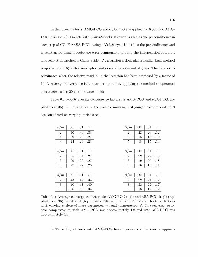
116

In the following tests, AMG-PCG and αSA-PCG are applied to (6.36). For AMG-

PCG, a single V(1,1)-cycle with Gauss-Seidel relaxation is used as the preconditioner in

each step of CG. For αSA-PCG, a single V(2,2)-cycle is used as the preconditioner and

is constructed using 4 prototype error components to build the interpolation operator.

The relaxation method is Gauss-Seidel. Aggregation is done algebraically. Each method

is applied to (6.36) with a zero right-hand side and random initial guess. The iteration is

terminated when the relative residual in the iteration has been decreased by a factor of

10−6. Average convergence factors are computed by applying the method to operators

constructed using 20 distinct gauge fields.

Table 6.1 reports average convergence factors for AMG-PCG and αSA-PCG, ap-

plied to (6.36). Various values of the particle mass m, and gauge field temperature β

are considered on varying lattice sizes.

β/m .001 .01 .1

2 .40 .39 .33

5 .29 .29 .27

3 .24 .24 .23

β/m .001 .01 .1

2 .35 .34 .27

3 .29 .29 .27

5 .27 .27 .26

β/m .001 .01 .1

2 .43 .42 .34

3 .40 .41 .40

5 .38 .38 .34

β/m .001 .01 .1

2 .22 .20 .12

3 .18 .18 .10

5 .15 .15 .14

β/m .001 .01 .1

2 .22 .22 .13

3 .19 .20 .18

5 .16 .15 .11

β/m .001 .01 .1

2 .22 .21 .12

3 .22 .22 .17

5 .18 .17 .12

Table 6.1: Average convergence factors for AMG-PCG (left) and αSA-PCG (right) ap-plied to (6.36) on 64 × 64 (top), 128 × 128 (middle), and 256 × 256 (bottom) latticeswith varying choices of mass parameter, m, and temperature, β. In each case, oper-ator complexity, σ, with AMG-PCG was approximately 1.8 and with αSA-PCG wasapproximately 1.4.

In Table 6.1, all tests with AMG-PCG have operator complexities of approxi-

117

mately 1.80, and with αSA-PCG have operator complexities of approximately 1.40. For

both solvers, the method performs better for the largest mass tested and slightly worse

for the two smaller masses. However, since performances remains fairly static between

m = .01 and m = .001 it appears that critical slowing down has been eliminated. The

value of β seems to affect the performance on both solvers. As the value of β increases

the matrix becomes easier to invert with both methods. This is not surprising, since a

larger β implies less disorder in the background gauge field. Finally, both solvers appear

to be scalable with respect to the lattice size.

To determine which solver is the most efficient we must consider convergence rates,

operator complexities, and types of V-cycle. The convergence rates reported in Table

6.1 are better for αSA-PCG than for AMG-PCG. Furthermore, the αSA V-cycle has

an operator complexity smaller than that of the AMG V-cycle, meaning that relaxation

sweeps and residual calculations are cheaper for αSA. However, αSA performs two more

relaxation steps on each level than AMG. To directly compare the two methods we again

compute their respective computational cost per digit of error reduction. These η-values

are given in Table 6.2.

β/m .001 .01 .1

2 13.6 13.2 11.2

3 10.0 10.0 9.5

5 8.7 8.7 8.5

β/m .001 .01 .1

2 10.6 10.0 7.6

3 9.4 9.4 7.0

5 8.5 8.5 8.2

Table 6.2: Average η-values for AMG-PCG (left) and αSA-PCG (right) applied to (6.36)on a 64× 64 lattice with varying choices of mass parameter m and temperature β.

Table 6.2 indicates that αSA-PCG performs better on (6.36) than AMG-PCG, but only

slightly. In fact, for simulations in which the discrete system need only be solved with

a few right-hand side vectors per gauge field, the larger setup costs of αSA may render

the method less efficient than AMG-PCG.

Again, it is interesting to compare the performance of an algebraic multigrid

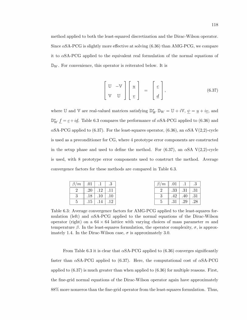
118

method applied to both the least-squared discretization and the Dirac-Wilson operator.

Since αSA-PCG is slightly more effective at solving (6.36) than AMG-PCG, we compare

it to αSA-PCG applied to the equivalent real formulation of the normal equations of

DW . For convenience, this operator is reiterated below. It is

U −V

V U

u

v

=

c

d

, (6.37)

where U and V are real-valued matrices satisfying D∗W DW = U + iV, ψ = u + iv, and

D∗W f = c+ id. Table 6.3 compares the performance of αSA-PCG applied to (6.36) and

αSA-PCG applied to (6.37). For the least-squares operator, (6.36), an αSA V(2,2)-cycle

is used as a preconditioner for CG, where 4 prototype error components are constructed

in the setup phase and used to define the method. For (6.37), an αSA V(2,2)-cycle

is used, with 8 prototype error components used to construct the method. Average

convergence factors for these methods are compared in Table 6.3.

β/m .01 .1 .3

2 .20 .12 .11

3 .18 .10 .10

5 .15 .14 .12

β/m .01 .1 .3

2 .33 .31 .31

3 .42 .40 .31

5 .31 .29 .28

Table 6.3: Average convergence factors for AMG-PCG applied to the least-squares for-mulation (left) and αSA-PCG applied to the normal equations of the Dirac-Wilsonoperator (right) on a 64 × 64 lattice with varying choices of mass parameter m andtemperature β. In the least-squares formulation, the operator complexity, σ, is approx-imately 1.4. In the Dirac-Wilson case, σ is approximately 3.0.

From Table 6.3 it is clear that αSA-PCG applied to (6.36) converges significantly

faster than αSA-PCG applied to (6.37). Here, the computational cost of αSA-PCG

applied to (6.37) is much greater than when applied to (6.36) for multiple reasons. First,

the fine-grid normal equations of the Dirac-Wilson operator again have approximately

88% more nonzeros than the fine-grid operator from the least-squares formulation. Thus,

119

all fine-grid computations are more expensive in the Dirac-Wilson case. Second, the

operator complexity associated with the Dirac-Wilson operator is 3.0 while the operator

complexity associated with the least-squares operator is only 1.4. The discrepancy

in operator complexity occurs for two reasons. First, the use of 8 prototype error

components for the Dirac-Wilson operator (versus 4 for least-squares) naturally yields

coarse grids with a greater number of unknowns. Second, because the normal equations

of the Dirac-Wilson operator must be solved, the stencil of the fine-grid operator is much

larger than the stencil of the least-squares operator. This leads to coarse-grid operators

with more connections between unknowns and, thus, more nonzeros in the coarse-grid

operators. To make a direct comparison between the two cases the appropriate η-values,

defined in (5.66) and (5.67), are compared. The results are reported in Table 6.4. The

associated speedup is reported in Table 6.5.

β/m .01 .1 .3

2 10.0 7.6 7.3

3 9.4 7.0 7.0

5 8.5 8.2 7.6

β/m .01 .1 .3

2 58.6 55.4 55.4

3 72.8 70.9 55.4

5 55.4 52.5 51.0

Table 6.4: Average ηLS and ηW -values for αSA-PCG applied to the least-squares dis-cretization and αSA-PCG applied to the normal equations of the Dirac-Wilson dis-cretization on a 64× 64 lattice with varying choices of mass parameter, m, and temper-ature, β.

β/m .01 .1 .3

2 5.8 7.3 7.6

3 8.0 10.1 7.9

5 6.5 6.4 6.7

Table 6.5: Average speedup factors for αSA-PCG applied to the least-squares discretiza-tion over αSA-PCG applied to the normal equations of the Dirac-Wilson discretizationon a 64× 64 lattice with varying choices of mass parameter, m, and temperature, β.

The speedups reported in Table 6.5 show that αSA-PCG applied to the least-

squares discretization attains between 5 and 10 times the reduction in error per work unit

120

than αSA-PCG applied to the normal equations of the Dirac-Wilson operator.

Chapter 7

Conclusions and Future Work

We conclude by reiterating the accomplishments of this thesis. We discuss the

long term goals using least-squares finite element methods to discretize the governing

equations of QED and QCD.

Chapters 1-3 serve as a general introduction to the Dirac equation for the applied

mathematician, both in the continuum and on the lattice. The full physical models of

QED and QCD are introduced, as well as the simpler 2D Schwinger model. Finally, an

alternate formulation of the 2D Schwinger model is introduced. Physical properties of

interest are defined and discussed for the continuum model, including gauge covariance

of the fermion propagator and chiral symmetry. These concepts are then extended to the

lattice setting. Two traditional discretizations of the governing equations are introduced

based on covariant finite-differences. These are the Naive and Dirac-Wilson discretiza-

tions. Through their development, the concept of species doubling is discovered and

discussed. We argue that both discretizations have serious problems, the Naive’s being

species doubling, and Wilson’s loss of chiral symmetry and very poor approximation

of the low modes of the continuum operator. A brief introduction to the least-squares

finite element methodology is presented in Chapter 4.

Chapter 5 develops a discretization of the 2D Schwinger model by applying the

least-squares methodology to the governing equations. It is quickly found that the

resulting discretization does not satisfy gauge covariance. To remedy this, the method

122

is altered, based on gauge fixing, to satisfy gauge covariance.

There are several advantages to discretizing the Schwinger model by least-squares

finite elements. First, the original governing equations are non-Hermitian. Thus,

straightforward discretization methods produce similarly non-Hermitian discrete op-

erators that are complicated to invert using multilevel methods. Using the least-squares

methodology avoids this problem because, by construction, the resulting discrete opera-

tor that must be inverted in the solution process is Hermitian positive semidefinite. This

allows the application standard algebraic multigrid techniques without serious modifi-

cation. Second, the principle part of the resulting operator has a 9-point Laplacian-like

stencil. Such an operator cannot have red-black instability and, thus, cannot suffer from

species doubling. This is perhaps the most fundamental benefit of the least-squares

methodology. By naturally avoiding species doubling, there is no need to add artificial

diffusion terms to the operator that break chiral symmetry and seriously damage the

spectrum of the discrete operator in the process. To see this, we compare the spectra

of the continuum, least-squares, and Dirac-Wilson operators. We show that the least-

squares operator, unlike the Dirac-Wilson operator, approximates the relevant parts of

the continuum spectrum very well.

Additionally, the least-squares functional is proved to be H1-elliptic. This al-

lows an additional argument that the discrete least-squares operator does not suffer

from species doubling. It also implies that an optimal multilevel method exists that

can efficiently solve the resulting system of equations. We investigate the use of alge-

braic multigrid preconditioned conjugate gradients (AMG-PCG) and adaptive smoothed

aggregation multigrid preconditioned conjugate gradients (αSA-PCG) as solution pro-

cesses for the resulting discrete system. Numerical experiments show that the discrete

least-squares operator can be solved efficiently using these methods. Furthermore, nei-

ther AMG-PCG nor αSA-PCG suffer from critical slowing down, and both scale well

with lattice size.

123

In Chapter 6, the least-squares methodology is applied to a transformation of

the 2D Schwinger operator. The transformation, based on a Helmholtz decomposition

of the gauge field, effectively removes the gauge field from the differential operator.

Then, applying least-squares yields a discrete operator similar to those obtained by

discretizing a variable-coefficient diffusion operator. This is very promising because

algebraic multigrid methods have proved to be highly effective at solving these types of

systems.

Again, gauge fixing is necessary to produce a gauge covariant solution process. As

in Chapter 5, we demonstrate that the discretization based on the transformed system

satisfies chiral symmetry while not suffering from species doubling. We also show that

the functional based on the transformed continuum operator satisfies H1-ellipticity in

a scaled H1-norm. We solve the resulting linear system using AMG-PCG and αSA-

PCG. Both methods perform very well, attaining convergence rates comparable to those

associated with Laplacian operators with variable coefficients. Finally, we compare the

solution of the discrete least-squares operator by AMG-PCG with the solution of the

Dirac-Wilson operator by αSA-PCG. We show that the solution of the former is roughly

seven times faster than the solution of the latter.

In summary, the main accomplishment of this thesis is the development of two

discretizations of the Schwinger model based on least-squares finite elements. Both

discretizations yield solution processes that retain gauge covariance and chiral symme-

try, while avoiding the problem of species doubling. Furthermore, both discretizations

agree very well spectrally with the continuum operator. Finally, both methods produce

Hermitian positive semidefinite linear systems of equations that can be solved very effec-

tively by algebraic multigrid methods. This is the first result to date that accomplishes

these goals without extending the theory to a costly extra dimension.

Although this thesis demonstrates that the least-squares methodology yields a

discretization of the Schwinger model with many nice properties, it is still based on

124

a simplified model. Extending it to the full physical model of either QED or QCD is

much more complicated. Though the form of the operators for the full QED model

are the same, extending a finite-element discretization to four dimensions is extremely

complicated. In QCD, gauge transformation are represented by objects in SU(3), which,

unlike objects in U(1), do not commute with one another. The lack of cancellation in

the formal normal means that a least-squares discretization of QCD yields a discrete

operator with many more nonzero entries. This, in and of itself, is not a serious problem

because the least-squares operator will not be any more dense than that of traditional

discretizations, but it may hinder the performance of multigrid solvers.

Finally, since there is no analytic solution of the governing equations for an ar-

bitrary gauge field, the only method of testing the viability of a discretization is to

incorporate it in a Monte Carlo simulation of the theory. Since this requires much more

knowledge of the physical theory, it is beyond the scope of this thesis. We are confi-

dent, though, based on our faithfulness to the original partial differential equation and

the agreement between the spectra of the discrete and continuum operators, that our

discretization methodology would be successful.

Bibliography

[1] J. Adler. Nested Iteration and FOSLS for Incompressible Resistive Magnetohydro-.dynamics. Ph.D. thesis, University of Colorado at Boulder, 2009.

[2] K. Atkinson. An Introduction to Numerical Analysis. John Wiley and Sons, 2ndedition, 1989.

[3] T. Austin and T. Manteuffel. A least-squares finite element method for the linearBoltzmann equation with anisotropic scattering. SIAM J. Numer. Anal., 44:540–560, 2006.

[4] M. Berndt, T. Manteuffel, and S. McCormick. Analysis of first-order system leastsquares (FOSLS) for elliptic problems with discontinuous coefficients: Part I. SIAMJ. Numer. Anal., 43:386, 2005.

[5] M. Berndt, T. Manteuffel, and S. McCormick. Analysis of first-order system leastsquares (FOSLS) for elliptic problems with discontinuous coefficients: Part II.SIAM J. Numer. Anal., 43:409, 2005.

[6] Z. Bochev, Z. Cai, T. Manteuffel, and S. McCormick. First-order system leastsquares principles for the Navier-Stokes Equations: Part I. SIAM J. Numer. Anal.,35:990–1009, 1998.

[7] Z. Bochev, Z. Cai, T. Manteuffel, and S. McCormick. First-order system leastsquares principles for the Navier-Stokes Equations: Part II. SIAM J. Numer.Anal., 36:1125–1144, 1999.

[8] D. Braess. Towards algebraic multigrid for elliptic problems of second order.Computing, 55:379–393, 1995.

[9] D. Braess. Finite Elements. Cambridge Univerity Press, Cambridge MA, 2ndedition, 2001.

[10] A. Brandt. personal communication, 2008.

[11] A. Brandt, S. McCormick, and J. Ruge. Algebraic multigrid (amg) for solutionwith application to geodetic computations. Sparsity and Its Applications, 1984.

[12] A. Brandt, S. McCormick, and J. Ruge. Algebraic multigrid (AMG) for sparsematrix equations. Sparsity and Its Applications, 1984.

126

[13] J. Brannick, M. Brezina, D. Keyes, O. Livne, I. Livshits, S. MacLachlan, T. Man-teuffel, S. McCormick, J. Ruge, and L. Zikatanov. Adaptive Smoothed Aggregationin Lattice QCD. Lecture Notes in Computational Science and Engineering, 55:507,2007.

[14] J. Brannick, J. C. Brower, M. A. Clark, T. Manteuffel, S. McCormick, J. C. Osborn,and C. Rebbi. The removal of critical slowing down. Submitted in Proceedings ofScience (PoS), Lat2008, 2008.

[15] J. Brannick, RC Brower, MA Clark, JC Osborn, and C. Rebbi. Adaptive MultigridAlgorithm for Lattice QCD. Physical Review Letters, 100(4):41601, 2008.

[16] J. Brannick, C. Ketelsen, T. Manteuffel, and S. McCormick. Least-squares finiteelement methods for quantum electrodynamics. SIAM J. Sci. Comp., 2009. Sub-mitted.

[17] S.C. Brenner and L.R. Scott. Mathematical Theory of Finite Element Methods.Springer, 2nd edition, 2002.

[18] M. Brezina, R. Falgout, S. MacLachlan, T. Manteuffel, S. McCormick, and J. Ruge.Adaptive smoothed aggregation (alphasa) multigrid. SIAM Review, 47(2):317,2005.

[19] M. Brezina, R. Falgout, S. MacLachlan, T. Manteuffel, S. McCormick, and J. Ruge.Adaptive algebraic multigrid. SIAM J. on Sci. Comp. (SISC), 27:1261–1286, 2006.

[20] M. Brezina, T. Manteuffel, S. McCormick, J. Ruge, and G. Sanders. Towardsadaptive smoothed aggregation (αsa) for nonsymmetric problems. SIAM J. Sci.Comp., 2008. Submitted.

[21] W. L. Briggs, V. E. Henson, and S. F. McCormick. A Multigrid Tutorial. Societyfor Industrial and Applied Mathematics (SIAM), Philadelphia, PA, 2000.

[22] R. C. Brower, C. Edwards, C. Rebbi, and E. Vicari. Projective multigrid for wilsonfermions. Nucl. Phys., B336(689), 1993.

[23] Z. Cai, R. Lazarov, T. Manteuffel, and S. McCormick. First-order system leastsquares for second-order partial differential equations: Part I. SIAM J. Numer.Anal., 31:1785, 1994.

[24] Z. Cai, T. Manteuffel, and S. McCormick. First-order system least squares forsecond-order partial differential equations: Part II. SIAM J. Numer. Anal., 34:425,1997.

[25] M. Clark. Quantum chromodynamics multigrid (qcdmg) software package. web-site: http://lattice.bu.edu/qcdmg. 2008.

[26] A. Codd, T. Manteuffel, and S. McCormick. Multilevel first-order system leastsquares for nonlinear elliptic partial differential equations. SIAM J. Numer. Anal.,41:2197–2209, 2003.

[27] M. Creutz. Quarks, Gluons and Lattices. Cambridge University Press, 1983.

127

[28] M. Creutz. Fun with Dirac eigenvalues. Arxiv preprint hep-lat/0511052, 2005.

[29] T. DeGrand and C. DeTar. Lattice Methods for Quantum Chromodynamics.World Scientific, 2006.

[30] R. G. Edwards. Numerical Simulations in Lattice Gauge Theories and Statistical.Mechanics. Ph.D. thesis, New York University, 1989.

[31] R. Friedberg, TD Lee, Y. Pang, and HC Ren. Noncompact lattice formulation ofgauge theories. Physical Review D, 52(7):4053–4081, 1995.

[32] D. Griffiths. Introduction to Elementary Particles. Wiley-VCH, 2004.

[33] M. Hestenes and E. Steifel. Methods of conjugate gradients for solving linearsystems. J. Research NBS, 49:400–436, 1952.

[34] J. K. Hunter and B. Nachtergaele. Applied Analysis. World Scientific, 2001.

[35] D. B. Kaplan. A method for simulating chiral fermions on the lattice. Phys. Lett.B, 288(342), 1992.

[36] C. Ketelsen, T. Manteuffel, S. McCormick, and J. Ruge. Finite element methodsfor quantum electrodynamics based on a helmholtz decomposition of the gaugefield. Num. Lin. Alg., 2009. Submitted.

[37] M. Lusher. Local coherence and deflation of low quark modes in lattice QCD. Phys.Lett. B, 417(141), 1998.

[38] M. Lusher. Local coherence and deflation of low quark modes in lattice QCD. HighEnergy Phys., 2007(81):1126–6708, 2007.

[39] S. MacLachlan. Improving Robustness in Multiscale Methods. Ph.D. thesis, Uni-versity of Colorado at Boulder, 2004.

[40] T. Manteuffel and K. Ressel. A least-squares finite element solution of the neutrontransport equation in diffusive regimes. SIAM J. Numer. Anal., 85:806–835, 1998.

[41] S. McCormick. Multilevel first-order system least squares (FOSLS) for Helmholtzequations. Procs. Conf. Maxwell Equations, 1993.

[42] J. C. Nedelec. A new family of mixed finite elements in R3. NumerischeMathematik, 50(1):57–81, 1986.

[43] C. W. Osterlee, A. Schuller, and U. Trottenberg. Multigrid. Academic Press, 2000.

[44] P.A. Raviart and J.M. Thomas. A mixed finite element method for second orderelliptic problems. Aspects of the Finite Element Method, Lectures Notes in Math.,606, 1977.

[45] C. Rebbi. Chiral-invariant regularization of fermions on the lattice. Physics LettersB, 186(2):200–204, 1987.

[46] O. Roehrle. Multilevel FOSLS Quasilinear Elliptic Partial Differential Equations.Ph.D. thesis, University of Colorado at Boulder, 2004.

128

[47] Y. Saad. Iterative Methods for Sparse Linear Systems. SIAM Books, 2003.

[48] Y. Shamir. Chiral fermions from lattice boundaries. Nucl. Phys., B406(90), 1993.

[49] P. Vanek, J. Mandel, and M. Brezina. Algebraic multigrid by smoothed aggregationfor second and fourth order elliptic problems. Computing, 56(3):179–196, 1996.

[50] P. Wesseling. Principles of Computational Fluid Dynamics. Springer, 2001.

[51] C. Westphal. FOSLS for Geometrically-Nonlinear Elasticity in Nonsmooth.Domains. Ph.D. thesis, University of Colorado at Boulder, 2004.

[52] K.G. Wilson. Confinement of quarks. Physical Review D, 10(8):2445–2459, 1974.

[53] A. Zee. Quantum Field Theory in a Nutshell. Princeton University Press, 2003.

[54] X. Zhang. Multilevel Schwarxz Methods. Numer. Math, 63:521–539, 1992.