learning with clustering structure - webhomeaspremon/pdf/supervisedclustering.pdf · learning with...
TRANSCRIPT

LEARNING WITH CLUSTERING STRUCTURE
VINCENT ROULET, FAJWEL FOGEL, ALEXANDRE D’ASPREMONT, AND FRANCIS BACH
ABSTRACT. We study supervised learning problems using clustering constraints to impose structure on eitherfeatures or samples, seeking to help both prediction and interpretation. The problem of clustering featuresarises naturally in text classification for instance, to reduce dimensionality by grouping words together andidentify synonyms. The sample clustering problem on the other hand, applies to multiclass problems wherewe are allowed to make multiple predictions and the performance of the best answer is recorded. We derive aunified optimization formulation highlighting the common structure of these problems and produce algorithmswhose core iteration complexity amounts to a k-means clustering step, which can be approximated efficiently.We extend these results to combine sparsity and clustering constraints, and develop a new projection algorithmon the set of clustered sparse vectors. We prove convergence of our algorithms on random instances, based ona union of subspaces interpretation of the clustering structure. Finally, we test the robustness of our methodson artificial data sets as well as real data extracted from movie reviews.
1. INTRODUCTION
Adding structural information to supervised learning problems can significantly improve prediction per-formance. Sparsity for example has been proven to improve statistical and practical performance [Bachet al., 2012]. Here, we study clustering constraints that seek to group either features or samples, to bothimprove prediction and provide additional structural insights on the data.
When there exists some groups of highly correlated features for instance, reducing dimensionality byassigning uniform weights inside each distinct group of features can be beneficial both in terms of predictionand interpretation [Bondell and Reich, 2008] by significantly reducing dimension. This often occurs in textclassification for example, where it is natural to group together words having the same meaning for a giventask [Dhillon et al., 2003; Jiang et al., 2011].
On the other hand, learning a unique predictor for all samples can be too restrictive. For recommendationsystems for example, users can be partitioned in groups, each having different tastes. Here, we study how tolearn a partition of the samples that achieves the best within-group prediction [Guzman-Rivera et al., 2014;Zhang, 2003]
These problems can of course be tackled by grouping synonyms or clustering samples in an unsupervisedpreconditioning step. However such partitions might not be optimized or relevant for the prediction task.Prior hypotheses on the partition can also be added as in Latent Dirichlet Allocation [Blei et al., 2003]or Mixture of Experts [Jordan, 1994]. We present here a unified framework that highlights the clusteredstructure of these problems without adding prior information on these clusters. While constraining thepredictors, our framework allows the use of any loss function for the prediction task. We propose severaloptimization schemes to solve these problems efficiently.
First, we formulate an explicit convex relaxation which can be solved efficiently using the conditionalgradient algorithm [Frank and Wolfe, 1956; Jaggi, 2013], where the core inner step amounts to solvinga clustering problem. We then study an approximate projected gradient scheme similar to the IterativeHard Thresholding (IHT) algorithm [Blumensath and Davies, 2009] used in compressed sensing. While
Date: September 19, 2016.Key words and phrases. Clustering, Multitask, Dimensionality Reduction, Supervised Learning, Supervised Clustering.A shorter, preliminary version of this paper appeared at the NIPS 2015 workshop “Transfer and Multi-Task Learning: Trends
and New Perspectives”.1

constraints are non-convex, projection on the feasible set reduces to a clustering subproblem akin to k-means.In the particular case of feature clustering for regression, the k-means steps are performed in dimension one,and can therefore be solved exactly by dynamic programming [Bellman, 1973; Wang and Song, 2011].When a sparsity constraint is added to the feature clustering problem for regression, we develop a newdynamic program that gives the exact projection on the set of sparse and clustered vectors.
We provide a theoretical convergence analysis of our projected gradient scheme generalizing the proofmade for IHT. Although our structure is similar to sparsity, we show that imposing a clustered structure,while helping interpretability, does not allow us to significantly reduce the number of samples, as in thesparse case for example.
Finally, we describe experiments on both synthetic and real datasets involving large corpora of text frommovie reviews. The use of k-means steps makes our approach fast and scalable while comparing veryfavorably with standard benchmarks and providing meaningful insights on the data structure.
2. LEARNING & CLUSTERING FEATURES OR SAMPLES
Given n sample points represented by the matrix X = (x1, . . . , xn)T ∈ Rn×d and corresponding labelsy = (y1, . . . , yn), real or nominal depending on the task (classification or regression), we seek to computelinear predictors represented by W . Clustering features or samples is done by constraining W and ourproblems take the generic form
minimize Loss(y,X,W ) +R(W )subject to W ∈ W,
in the prediction variable W , where Loss(y,X,W ) is a learning loss (for simplicity, we consider onlysquared or logistic losses in what follows), R(W ) is a classical regularizer and W encodes the clusteringstructure.
The clustering constraint partitions features or samples into Q groups G1, . . . ,GQ of size s1, . . . , sQ byimposing that all features or samples within a cluster Gq share a common predictor vector or coefficientvq, solving the supervised learning problem. To define it algebraically we use a matrix Z that assigns thefeatures or the samples to the Q groups, i.e. Ziq = 1 if feature or sample i is in group Gq and 0 otherwise.Denoting V = (v1, . . . , vQ), the prediction variable is decomposed as W = ZV leading to the supervisedlearning problem with clustering constraint
minimize Loss(y,X,W ) +R(W )subject to W = ZV, Z ∈ 0, 1m×Q, Z1 = 1,
(1)
in variables W , V and Z whose dimensions depend on whether features (m = d) or samples (m = n) areclustered.
Although this formulation is non-convex, we observe that the core non-convexity emerges from a clus-tering problem on the predictors W , which we can deal with using k-means approximations, as detailed inSection 3. We now present in more details two key applications of our formulation: dimensionality reductionby clustering features and learning experts by grouping samples. We only detail regression formulations,extensions for classification are given in the Appendix 7.1. Our framework also applies to clustered mul-titask as a regularization hypothesis, and we refer the reader to the Appendix 7.2 for more details on thisformulation.
2.1. Dimensionality reduction: clustering features. Given a prediction task, we want to reduce dimen-sionality by grouping together features which have a similar influence on the output [Bondell and Reich,2008], e.g. synonyms in a text classification problem. The predictor variable W is here reduced to a singlevector, whose coefficients take only a limited number of values. In practice, this amounts to a quantizationof the classifier vector, supervised by a learning loss.
2

Our objective is to form Q groups of features G1, . . . ,GQ, assigning a unique weight vq to all features ingroup Gq. In other words, we search a predictor w ∈ Rd such that wj = vq for all j ∈ Gq. This problem canbe written
minimize 1n
∑ni=1 loss
(yi, w
Txi)
+ λ2‖w‖22
subject to w = Zv, Z ∈ 0, 1d×Q, Z1 = 1,(2)
in the variables w ∈ Rd, v ∈ RQ and Z. In what follows, loss(yi, wTxi) will be a squared or logistic lossthat measures the quality of prediction for each sample. Regularization can either be seen as a standard l2regularization on w with R(w) = λ
2‖w‖22, or a weighted regularization on v, R(v) = λ2
∑Qq=1 sq‖vq‖22.
Note that fused lasso [Tibshirani et al., 2005] in dimension one solves a similar problem that also quan-tizes the regression vector using an `1 penalty on coefficient differences. The crucial difference with oursetting is that fused lasso assumes that the variables are ordered and minimizes the total variation of thecoefficient vector. Here we do not make any ordering assumption on the regression vector.
2.2. Learning experts: clustering samples. Mixture of experts [Jordan, 1994] is a standard model forprediction that seeks to learn Q predictors called “experts”, each predicting labels for a different group ofsamples. For a new sample x the prediction is then given by a weighted sum of the predictions of all expertsy =
∑Qq=1 pqv
Tq x. The weights pq are given by a prior probability depending on x. Here, we study a slightly
different setting where we also learn Q experts, but assignments to groups are only extracted from the labelsy and not based on the feature variables x as illustrated by the graphical model in Figure 1.
162163164165166167168169170171172173174175176177178179180181182183184185186187188189190191192193194195196197198199200201202203204205206207208209210211212213214215
patients different treatments were given. Since patients are uniformly distributed, the groups cannotbe predicted without supplementary information. We will use the effect of treatments to simultane-ously retrieve the groups of patients and the associated regression functions. Note that this setting isdifferent from a mixture of experts model in the sense that the latent cluster assignment variable Zcan only be estimated once y is known and cannot be deduced from the input features X .
Z
X Y
Z
X Y
Figure 2: Learning multiple diverse predictors (left), mixture of experts model (right).
Given a regression or multi-classification task, we want to find Q groups of sample points to max-imize the within-group prediction performance using a group specific predictor. This amount toproducing Q diverse answers per sample point, considering only the best one. We thus learn Q pre-dictors, each predictor having low error rate on some cluster of points. For simplicity, we illustratethe case of regression, which can be extended to multi-classification. We minimize the loss incurredby the best linear predictor fq : x! cT
q x for each point, i.e.
L(V ) = L(CZT ) =1
n
nX
i=1
minq21,...,Q
l(yi, cTq xi) =
1
n
nX
i=1
l
yi,
QX
q=1
ZiqcTq xi
!,
in the matrix variable V 2 Rdn of predictor vectors (one per sample point), where C 2 RdQ andZ 2 0, 1nQ are the centroid and assignment matrices defined above.
Loss Dim. U, V Predictors GoalFeatures 1
n
Pni=1 l
PQq=1
Pdj=1 Zjqcqxij
1 d rows of W regression
Tasks 1n
PKk=1
Pni=1 l(wT
k xi) dK columns of W classification
Samples 1n
Pni=1 l
PQq=1 Ziqc
Tq xi
d n W (i) regression
Table 1: Summary of the presented supervised clustering settings.
3 Algorithms
We now present optimization strategies to solve these supervised clustering problems. We begin bysimple greedy procedures, then propose a non-convex projected gradient descent scheme and finallya more refined convex relaxation solved using conditional gradient and approximations to k-means.
3.1 Simple strategies
A straightforward strategy is to first minimize on predictors, as in a classical supervised learningproblem, and then cluster predictors together using k-means. The procedure can be repeated in thecase of a soft clustering penalty. In the same spirit, when clustering sample points, one can alternateminimization on the predictors of each group and assignment of each point to the group whereits loss is smallest. These methods are fast but very dependent on the initialization. Alternatingminimization can optionally be used to refine the solution of the more robust algorithms proposedbelow.
3.2 Projected gradient descent
A natural strategy is to do a projected gradient descent on the non-convex problems (HSC) or (SSC).The projection of a matrix V is made by finding
argminZ,C
kV CZT k2F = argmin
QX
q=1
X
i2Cq
kvi cqk22,
4
FIGURE 1. Learning multiple diverse experts (left), mixture of experts model (right). Theassignment matrix Z gives the assignment to groups, grey variables are observed, arrowsrepresent dependance of variables.
This means that while we learn several experts (classifier vectors), the information contained in the fea-tures x is not sufficient to select the best experts. Given a new point x we can only give Q diverse answersor an approximate weighted prediction y =
∑Qq=1
sqn v
Tq x. Our algorithm will thus return several answers
and minimizes the loss of the best of these answers. This setting was already studied by Zhang [2003] forgeneral predictors, it is also related to subspace clustering [Elhamifar and Vidal, 2009], however here wealready know in which dimension the data points lie.
Given a prediction task, our objective is to find Q groups G1, . . . ,GQ of sample points to maximizewithin-group prediction performance. Within each group Gq, samples are predicted using a common linearpredictor vq. Our problem can be written
minimize1
n
Q∑
q=1
∑
i∈Gq
loss(yi, v
Tq xi)
+λ
2
Q∑
q=1
sq‖vq‖22 (3)
in the variables V = (v1, . . . , vQ) ∈ Rd×Q and G = (G1, . . . ,GQ) such that G is a partition of the nsamples. As in the problem of clustering features above, loss(yi, vTq xi) measures the quality of predictionfor each sample and R(V ) = λ
2
∑Qq=1 sq‖vq‖22 is a weighted regularization. Using an assignment matrix
Z ∈ 0, 1n×Q and an auxiliary variable W = (w1, . . . , wn) ∈ Rd×n such that W = V ZT , which means3

wi = vq if i ∈ Gq, problem (3) can be rewritten
minimize 1n
∑ni=1 loss
(yi, w
Ti xi)
+ λ2
∑ni=1 ‖wi‖22
subject to W T = ZV T , Z ∈ 0, 1n×Q, Z1 = 1,
in the variables W ∈ Rd×n, V ∈ Rd×Q and Z. Once again, our problem fits in the general formulationgiven in (1) and in the sections that follows, we describe several algorithms to solve this problem efficiently.
3. APPROXIMATION ALGORITHMS
We now present optimization strategies to solve learning problems with clustering constraints. We beginby simple greedy procedures and a more refined convex relaxation solved using approximate conditionalgradient. We will show that this latter relaxation is exact in the case of feature clustering because the innerone dimensional clustering problem can be solved exactly by dynamic programming.
3.1. Greedy algorithms. For both clustering problems discussed above, greedy algorithms can be derivedto handle the clustering objective. A straightforward strategy to group features is to first train predictors asin a classical supervised learning problem, and then cluster weights together using k-means. In the samespirit, when clustering sample points, one can alternate minimization on the predictors of each group andassignment of each point to the group where its loss is smallest. These methods are fast but unstable andhighly dependent on initialization. However, alternating minimization can be used to refine the solution ofthe more robust algorithms proposed below.
3.2. Convex relaxation using conditional gradient algorithm. Another approach is to relax the problemby considering the convex hull of the feasible set and use the conditional gradient method (a.k.a. Frank-Wolfe, [Frank and Wolfe, 1956; Jaggi, 2013]) on the relaxed convex problem. Provided that an affineminimization oracle can be computed efficiently, the key benefit of using this method when minimizing aconvex objective over a non-convex set is that it automatically solves a convex relaxation, i.e. minimizesthe convex objective over the convex hull of the feasible set, without ever requiring this convex hull to beformed explicitly.
In our case, the convex hull of the set W : W = ZV, Z ∈ 0, 1m×Q, Z1 = 1 is the entire spaceso the relaxed problem loses the initial clustering structure. However in the special case of a squared loss,i.e. loss(y, y) = 1
2(y − y)2, minimization in V can be performed analytically and our problem reducesto a clustering problem for which this strategy is relevant. We illustrate this simplification in the case ofclustering features for a regression task, detailed computations and explicit procedures for other settings aregiven in Appendix 7.3.
Replacing w = Zv in (2), the objective function in problem (2) becomes
φ(v, Z) =1
2n
n∑
i=1
(yi − (Zv)T xi
)2+λ
2‖Zv‖22
=1
2nvTZTXTXZv +
λ
2vTZTZv − 1
nyTXZv +
1
2nyT y.
Minimizing in v and using the Sherman-Woodbury-Morrison formula we then get
minvφ(v, Z) =
1
2nyT(I−XZ(ZTXTXZ + λnZTZ)−1ZTXT
)y
=1
2nyT(I +
1
nλXZ(ZTZ)−1ZTXT
)−1
y,
and the resulting clustering problem is then formulated in terms of the normalized equivalence matrix
M = Z(ZTZ)−1ZT
such that Mij = 1/sq if item i and j are in the same group Gq and 0 otherwise.4

WritingM = M : M = Z(ZTZ)−1ZT , Z ∈ 0, 1d×Q, Z1 = 1 the set of equivalence matrices forpartitions into at most Q groups, our partitioning problem can be written
minimize ψ(M) , yT(I + 1
nλXMXT)−1
ysubject to M ∈M.
in the matrix variable M ∈ Sn. We now relax this last problem by solving it (implicitly) over the convexhull of the set of equivalence matrices using the conditional gradient method. Its generic form is describedin Algorithm (1), where the scalar product is the canonical one on matrices, i.e. 〈A,B〉 = Tr(ATB). Ateach iteration, the algorithm requires solving an linear minimization oracle over the feasible set. This givesthe direction for the next step and an estimated gap to the optimum which is used as stopping criterion.
Algorithm 1 Conditional gradient algorithmInitialize M0 ∈Mfor t = 0, . . . , T do
Solve linear minimization oracle
∆t = argminN∈hull(M)
〈N,∇ψ(Mt)〉 (4)
if gap(Mt,M∗) ≤ ε thenreturn Mt
elseSet Mt+1 = Mt + αt(∆t −Mt)
end ifend for
The estimated gap is given by the linear oracle as
gap(Mt,M∗) , −〈∆t −Mt,∇ψ(Mt)〉.By definition of the oracle and convexity of the objective function, we have
−〈∆t −Mt,∇ψ(Mt)〉 ≥ −〈M∗ −Mt,∇ψ(Mt)〉 ≥ ψ(Mt)− ψ(M∗).
Crucially here, the linear minimization oracle in (4) is equivalent to a projection step. This projection step isitself equivalent to a k-means clustering problem which can be solved exactly in the feature clustering caseand well approximated in the other scenarios detailed in the appendix. For a fixed matrix M ∈ hull(M),we have that
P , −∇ψ(M) =1
2n2λXT (I +
1
nλXMXT )−1 y yT (I +
1
nλXMXT )−1X
is positive semidefinite (this is the case for all the settings considered in this paper). Writing P12 its matrix
square root we get
argminN∈hull(M)
〈N,∇ψ(M)〉 = argminN∈M
Tr(NT∇ψ(M))
= argminN∈M
−Tr(NP12P
12T
)
= argminN∈M
Tr((I−N)P12P
12T
))
= argminN∈M
‖P 12 −NP 1
2 ‖2F
= argminZ
minV‖P 1
2 − ZV ‖2F ,5

because N is an orthonormal projection (N2 = N , NT = N ) and so is (I − N). Given a matrix W , wealso have
argminZ,V
‖W − ZV ‖2F = argmin
Q∑
q=1
∑
i∈Gq
‖wi − vq‖22, (5)
where the minimum is taken over centroids vq and partition (G1, . . . ,GQ). This means that computingthe linear minimization oracle on ∇ψ(M) is equivalent to solving a k-means clustering problem on P 1/2.This k-means problem can itself be solved approximately using the k-means++ algorithm which performsalternate minimization on the assignments and the centroids after an appropriate random initialization. Al-though this is a non-convex subproblem, k-means++ guarantees a constant approximation ratio on its solu-tion [Arthur and Vassilvitskii, 2007]. We write k-means(V,Q) the approximate solution of the projection.Overall, this means that the linear minimization oracle (4) can therefore be computed approximately. More-over, in the particular case of grouping features for regression, the k-means subproblem is one-dimensionaland can be solved exactly using dynamic programming [Bellman, 1973; Wang and Song, 2011] so thatconvergence of the algorithm is ensured.
The complete method is described as Algorithm 2 where we use the classical stepsize for conditionalgradient αt = 2
t+2 . A feasible solution for the original non-convex problem is computed from the solutionof the relaxed problem using Frank-Wolfe rounding, i.e. output the last linear oracle.
Algorithm 2 Conditional gradient on the equivalence matrixInput: X, y,Q, ε
Initialize M0 ∈Mfor t = 0, . . . , T do
Compute the matrix square root P12 of −∇ψ(M0)
Get oracle ∆t = k-means(P12 , Q)
if −Tr(∆t −Mt)T∇ψ(Mt) ≤ ε then
return Mt
elseSet Mt+1 = Mt + αt(∆t −Mt)
end ifend forZ∗ is given by the last k-meansV ∗ is given by the analytic solution of the minimization for Z∗ fixed
Output: V ∗, Z∗
3.3. Complexity. The core complexity of Algorithm 2 is concentrated in the inner k-means subproblem,which standard alternating minimization approximates at cost O(tKQp), where tK is the number of alter-nating steps,Q is the number of clusters, and p is the product of the dimensions of V . However, computationof the gradient requires to invert matrices and to compute a matrix square root of the gradient at each iter-ation, which can slow down computations for large datasets. The choice of the number of clusters can bedone given an a priori on the problem (e.g. knowing the number of hidden groups in the sample points), orcross-validation, idem for the other regularization parameters.
4. PROJECTED GRADIENT ALGORITHM
In practice, convergence of the conditional gradient method detailed above can be quite slow and we alsostudy a projected gradient algorithm to tackle the generic problem in (1). Although simple and non-convexin general, this strategy used in the context of sparsity can produce scalable and convergent algorithms incertain scenarios, as we will see below.
6

4.1. Projected gradient. We can exploit the fact that projecting a matrix W on the feasible set
W : W = ZV, Z ∈ 0, 1m×Q, Z1 = 1is equivalent to a clustering problem, with
argminZ,V
‖W − ZV ‖2F = argmin
Q∑
q=1
∑
i∈Gq
‖wi − vq‖22,
where the minimum is taken over centroids vq and partition (G1, . . . ,GQ). The k-means problem can besolved approximately with the k-means++ algorithm as mentioned in Section 3.2. We will analyze thisalgorithm for clustering features for regression in which the projection can be found exactly. Writing k-means(V,Q) the approximate solution of the projection, φ the objective function and αt the stepsize, thefull method is summarized as Algorithm 3 and its implementation is detailed in Section 4.3.
Algorithm 3 Proj. Gradient DescentInput: X, y,Q, ε
Initialize W0 = 0while |φ(Wt)− φ(Wt−1)| ≥ ε doWt+ 1
2= Wt − αt(∇Loss(y,X,Wt) +∇R(Wt))
[Zt+1, Vt+1] = k-means(Wt+ 12, Q)
Wt+1 = Zt+1Vt+1
end whileZ∗ and V ∗ are given through k-means
Output: W ∗, Z∗, V ∗
4.2. Convergence. We now analyze the convergence of the projected gradient algorithm with a constantstepsize αt = 1, applied to the feature clustering problem for regression. We focus on a problem withsquared loss without regularization term, which reads
minimize 12n‖Xw − y‖22
subject to w = Zv, Z ∈ 0, 1d×Q, Z1 = 1
in the variables w ∈ Rd, v ∈ RQ and Z. We assume that the regression values y are generated by a linearmodel whose coefficients w∗ satisfy the constraints above, up to additive noise, with
y = Xw∗ + η
where η ∼ N (0, σ2). Hence we study convergence of our algorithm to w∗, i.e. to the partition G∗ of itscoefficients and its Q values.
We will exploit the fact that each partition G defines a subspace of vectors w, so the feasible set can bewritten as a union of subspaces. Let G be a partition and define
UG = w : w = Zv, Z ∈ Z(G),where Z(G) is the set of assignment matrices corresponding to G. Since permuting the columns of Ztogether with the coefficients of v has no impact onw, the matrices inZ(G) are identical up to a permutationof their columns. So, for Z ∈ Z(G), Z(G) = ZΠ,Π permutation matrix, therefore UG is a subspace andthe corresponding assignment matrices are its different basis.
To a feasible vector w, we associate the partition G of its values that has the least number of groups.This partition and its corresponding subspace are uniquely defined and, denoting P the set of partitions inat most Q clusters, our problem (6) can thus be written
minimize 12n‖Xw − y‖22
subject to w ∈ ⋃G∈P UG .7

where the variable w ∈ Rd belongs to a union of subspaces UG .We will write the projected gradient algorithm for (6) as a fixed point algorithm whose contraction factor
depends on the singular values of the design matrix X on collections of subspaces generated by the parti-tions G. We only need to consider largest subspaces in terms of inclusion order, which are the ones generatedby the partitions into exactly Q groups. Denoting PQ this set of partitions, the collections of subspaces aredefined as
E1 = UG , G ∈ PQ,E2 = UG1 +UG2 , (G1,G2) ∈ PQ,E3 = UG1 +UG2 +UG3 , (G1,G2,G3) ∈ PQ.
Our main convergence result follows. Provided that the contraction factor is sufficient, it states the con-vergence of the projected gradient scheme to the original vector up to a constant error of the order of thenoise.
Proposition 4.1. Given that projection on⋃G∈P UG is well defined, the projected gradient algorithm ap-
plied to (3) converges to the original w∗ as
‖w∗ − wt‖2 ≤ ρt‖w∗‖2 +1− ρt1− ρ ν‖η‖2,
where
ρ , 2 maxU∈E3
‖I − 1
nΠTUX
TXΠU‖2
ν ,2
nmaxU∈E2
‖XΠU‖2
and ΠU is any orthonormal basis of the subspace U .
Proof. To describe the algorithm we define Gt and G∗ as the partitions associated respectively with wtand w∗ containing the least number of groups and
wt+1/2 = wt −∇Loss(X, y,wt) = wt − 1nX
TX(wt − w∗) + 1nX
T η
wt+1 = argminw∈⋃G∈P UG ‖w − wt+1/2‖22
U t = UGtU t,∗ = UGt +UG∗U t,t+1,∗ = UGt +UGt+1 +UG∗ .
Orthonormal projections on U t, U t,∗ and U t,t+1,∗ are given respectively by Pt, Pt,∗, Pt,t+1,∗. Therefore bydefinition wt ∈ U t, (wt, w
∗) ∈ U t,∗ and (wt, wt+1, w∗) ∈ U t,t+1,∗.
We can now control convergence, with
‖w∗ − wt+1‖2 = ‖Pt+1,∗(w∗ − wt+1)‖2
≤ ‖Pt+1,∗(w∗ − wt+1/2)‖2 + ‖Pt+1,∗(wt+1/2 − wt+1)‖2. (6)
In the second term, as w∗ ∈ ⋃G∈P UG and wt+1 = argminw∈⋃G∈P UG ‖w − wt+1/2‖2, we have
‖wt+1 − wt+1/2‖22 ≤ ‖w∗ − wt+1/2‖22which is equivalent to
‖Pt+1,∗(wt+1 −wt+1/2)‖22 + ‖(I − Pt+1,∗)wt+1/2‖22 ≤ ‖Pt+1,∗(w∗ −wt+1/2)‖22 + ‖(I − Pt+1,∗)wt+1/2‖22
and this last statement implies
‖Pt+1,∗(wt+1 − wt+1/2)‖2 ≤ ‖Pt+1,∗(w∗ − wt+1/2)‖2.
8

This means that we get from (6)
‖w∗ − wt+1‖2 ≤ 2‖Pt+1,∗(w∗ − wt+1/2)‖2
= 2‖Pt+1,∗(w∗ − wt −
1
nXTX(w∗ − wt)−
1
nXT η)‖2
≤ 2‖Pt+1,∗(I −1
nXTX)(w∗ − wt)‖2 +
2
n‖Pt+1,∗(X
T η)‖2
= 2‖Pt+1,∗(I −1
nXTX)Pt,∗(w
∗ − wt)‖2 +2
n‖Pt+1,∗(X
T η)‖2
≤ 2‖Pt+1,∗(I −1
nXTX)Pt,∗‖2‖w∗ − wt‖2 +
2
n‖Pt+1,∗X
T ‖2‖η‖2.
Now, assuming
2‖Pt+1,∗(I −1
nXTX)Pt,∗‖2 ≤ ρ (7)
2
n‖Pt+1,∗X
T ‖2 ≤ ν (8)
and summing the latter inequality over t, using that w0 = 0, we get
‖w∗ − wt‖2 ≤ ρt‖w∗‖2 +1− ρt1− ρ ν‖η‖2.
We bound ρ and ν using the information of X on all possible subspaces of E2 or E3. For a subspace U ∈ E2
or E3, we define PU the orthonormal projection on it and ΠU any orthonormal basis of it. For (8) we get
‖Pt+1,∗XT ‖2 = ‖XPt+1,∗‖2 ≤ max
U∈E2‖XPU‖2 = max
U∈E2‖XΠU‖2,
which is independent of the choice of ΠU .For (7), using that U t,∗ ⊂ U t,t+1,∗ and U t+1,∗ ⊂ U t,t+1,∗, we have
‖Pt+1,∗(I −XTX)Pt,∗‖2 ≤ ‖Pt,t+1,∗(I −1
nXTX)Pt,t+1,∗‖2
≤ maxU∈E3
‖PU (I − 1
nXTX)PU‖2
= maxU∈E3
‖ΠU (I − 1
nΠTUX
TXΠU )ΠTU‖2
= maxU∈E3
‖I − 1
nΠTUX
TXΠU‖2,
which is independent of the choice of ΠU and yields the desired result. We now show that ρ and ν derive
from bounds on the singular values of X on the collections E2 and E3. Denoting smin(A) and smax(A)respectively the smallest and largest singular values of a matrix A, we have
maxU∈E2
‖XΠU‖2 = maxU∈E2
smax(XΠU ),
and assuming U ∈ E3 and that
1− δ ≤ smin(XΠU√n
)≤ smax
(XΠU√n
)≤ 1 + δ,
for some δ > 0, then [Vershynin, 2010, Lemma 5.38] shows
‖I − 1
nΠTUX
TXΠU‖2 ≤ 3 maxδ, δ2.9

We now show that for isotropic independent sub-Gaussian data xi, these singular values depend on thenumber of subspaces of E1, N , their dimension D and the number of samples n. This proposition reformu-lates results of Vershynin [2010] to exploit the union of subspace structure.
Proposition 4.2. Let E1, E2, E3 be the finite collections of subspaces defined above, letD = maxU∈E1 dim(U)and N = Card(E1). Assuming that the rows xi of the design matrix are n isotropic independent sub-gaussian, we have
1√n
maxU∈E2
‖XΠU‖2 ≤ 1 + δ2 + ε and maxU∈E3
‖I − 1
nΠTUX
TXΠU‖2 ≤ 3 maxδ3 + ε, (δ3 + ε)2,
with probability larger than 1− exp(−cε2n), where δp = C0
√pDn +
√1+p log(N)
cn , ΠU is any orthonormalbasis of U and C0, c depend only on the sub-gaussian norm of the xi.
Proof. Let us fix U ∈ Ep, with p = 2 or 3 and ΠU one of its orthonormal basis. By definition of Ep,dim(U) ≤ pD. The rows of XΠU are orthogonal projections of the rows of X onto U , so they are stillindependent sub-gaussian isotropic random vectors. We can therefore apply [Vershynin, 2010, Theorem5.39] on XΠU ∈ Rn×dim(U). Hence for any s ≥ 0, with probability at least 1 − 2 exp(−cs2), the smallestand largest singular values of the rescaled matrix XΠU√
nwritten respectively smin(XΠU√
n) and smax(XΠU√
n) are
bounded by
1− C0
√pD
n− s√
n≤ smin
(XΠU√n
)≤ smax
(XΠU√n
)≤ 1 + C0
√pD
n+
s√n, (9)
where c and C0 depend only on the sub-gaussian norm of the xi. Now taking the union bound on all subsetsof Ep, (9) holds for any U ∈ Ep with probability
1− 2
(N
p
)exp(−cs2) ≥ 1− 2
(eN
p
)pexp(−cs2)
≥ 1− 2 exp(1 + p log(N)− cs2).
Taking s =
√1+p log(N)
c + ε√n, we get for all U ∈ Ep,
1− δp − ε ≤ smin(XΠU√n
)≤ smax
(XΠU√n
)≤ 1 + δp + ε,
with probability at least 1− exp(−cε2n), where δp = C0
√pDn +
√1+p log(N)
cn . Therefore
1√n
maxU∈E2
‖XΠU‖2 ≤ 1 + δ2 + ε.
Then [Vershynin, 2010, Theorem 5.39] yields
maxU∈E3
‖I − 1
nΠTUX
TXΠU‖2 ≤ 3 maxδ3 + ε, (δ3 + ε)2,
hence the desired result.
Overall here, Proposition 4.1 shows that the projected gradient method converges when the contractionfactor ρ is strictly less than one. When observations xi are isotropic independent sub-gaussian, this means
C0
√3D
n<
1
3and
√1 + 3 log(N)
cn<
1
3
which is alson = Ω(D) and n = Ω(log(N)) (10)
10
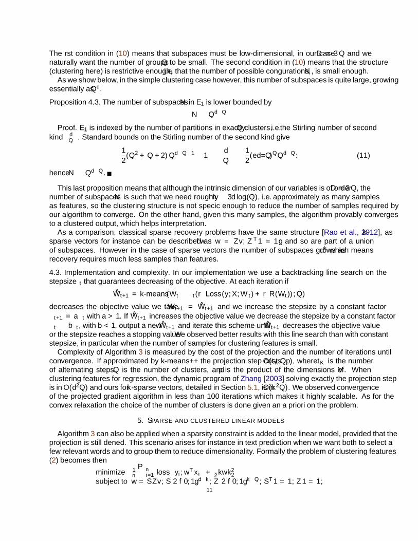
The first condition in (10) means that subspaces must be low-dimensional, in our case D = 3Q and wenaturally want the number of groups Q to be small. The second condition in (10) means that the structure(clustering here) is restrictive enough, i.e. that the number of possible configurations, N , is small enough.
As we show below, in the simple clustering case however, this number of subspaces is quite large, growingessentially as Qd.
Proposition 4.3. The number of subspaces N in E1 is lower bounded by
N ≥ Qd−Q
Proof. E1 is indexed by the number of partitions in exactly Q clusters, i.e.the Stirling number of secondkind
dQ
. Standard bounds on the Stirling number of the second kind give
1
2(Q2 +Q+ 2)Qd−Q−1 − 1 ≤
d
Q
≤ 1
2(ed/Q)QQd−Q. (11)
hence N ≥ Qd−Q.
This last proposition means that although the intrinsic dimension of our variables is of orderD = 3Q, thenumber of subspaces N is such that we need roughly n ≥ 3d log(Q), i.e. approximately as many samplesas features, so the clustering structure is not specific enough to reduce the number of samples required byour algorithm to converge. On the other hand, given this many samples, the algorithm provably convergesto a clustered output, which helps interpretation.
As a comparison, classical sparse recovery problems have the same structure [Rao et al., 2012], as k-sparse vectors for instance can be described as w : w = Zv, ZT 1 = 1 and so are part of a “unionof subspaces”. However in the case of sparse vectors the number of subspaces grows as dk which meansrecovery requires much less samples than features.
4.3. Implementation and complexity. In our implementation we use a backtracking line search on thestepsize αt that guarantees decreasing of the objective. At each iteration if
Wt+1 = k-means (Wt − αt(∇Loss(y,X,Wt) +∇R(Wt)), Q)
decreases the objective value we take Wt+1 = Wt+1 and we increase the stepsize by a constant factorαt+1 = aαt with a > 1. If Wt+1 increases the objective value we decrease the stepsize by a constant factorαt ← bαt, with b < 1, output a new Wt+1 and iterate this scheme until Wt+1 decreases the objective valueor the stepsize reaches a stopping value ε. We observed better results with this line search than with constantstepsize, in particular when the number of samples for clustering features is small.
Complexity of Algorithm 3 is measured by the cost of the projection and the number of iterations untilconvergence. If approximated by k-means++ the projection step costs O(tKQp), where tK is the numberof alternating steps, Q is the number of clusters, and p is the product of the dimensions of V . Whenclustering features for regression, the dynamic program of Zhang [2003] solving exactly the projection stepis in O(d2Q) and ours for k-sparse vectors, detailed in Section 5.1, is in O(k2Q). We observed convergenceof the projected gradient algorithm in less than 100 iterations which makes it highly scalable. As for theconvex relaxation the choice of the number of clusters is done given an a priori on the problem.
5. SPARSE AND CLUSTERED LINEAR MODELS
Algorithm 3 can also be applied when a sparsity constraint is added to the linear model, provided that theprojection is still defined. This scenario arises for instance in text prediction when we want both to select afew relevant words and to group them to reduce dimensionality. Formally the problem of clustering features(2) becomes then
minimize 1n
∑ni=1 loss
(yi, w
Txi)
+ λ2‖w‖22
subject to w = SZv, S ∈ 0, 1d×k, Z ∈ 0, 1k×Q, ST1 = 1, Z1 = 1,11

in the variables w ∈ Rd, v ∈ RQ, S and Z, where S is a matrix of k canonical vectors which assignsnonzero coefficients and Z an assignment matrix of k variables in Q clusters.
We develop a new dynamic program to get the projection on k-sparse vectors whose non-zero coefficientsare clustered in Q groups and apply our previous theoretical analysis to prove convergence of the projectedgradient scheme on random instances.
5.1. Projection on k-sparse Q-clustered vectors. Let W be the set of k-sparse vectors whose non-zerovalues can be partitioned in at most Q groups. Given x ∈ Rd, we are interested in its projection on W ,which we formulate as a partitioning problem. For a feasible w ∈ W , with G0 = i : wi = 0 andG1, . . . ,GQ′ , with Q′ ≤ Q, the partition of its non-zero values such that wi = vq if and only if i ∈ Gq, thedistance between x and w is given by
‖x− w‖22 =∑
i∈G0
x2i +
Q′∑
q=1
∑
i∈Gq
(xi − vq)2.
The projection is solution of
minimize∑
i∈G0 x2i +
∑Q′
q=1
∑i∈Gq(xi − vq)2
subject to Card(⋃Q′
q=1 Gq)≤ k, 0 ≤ Q′ ≤ Q, (12)
in the number of groups Q′, the partition G = (G0, . . . ,GQ′) of 1, . . . , d and v ∈ RQ′ . For a fixed numberof non-zero values k′, the objective is clearly decreasing in the number of groups Q′, which measures thedegrees of freedom of the projection, however it cannot exceed k′. We will use this argument below to getthe best parameter Q′. For a fixed partition G, minimization in v gives the barycenters of the Q′ groups,µq = 1
sq
∑i∈Gq xi. Inserting them in (12), the objective can be developed as
∑
i∈G0
x2i +
Q′∑
q=1
∑
i∈Gq
x2i + µ2
q − 2µqxi =d∑
i=1
x2i −
Q′∑
q=1
sqµ2q .
Splitting this objective between positive and negative barycenters, we get that the minimizer of (12) solves
maximize∑
q : µq<0 sqµ2q +
∑q : µq>0 sqµ
2q
subject to Card(⋃Q′
q=1 Gq)≤ k, 0 ≤ Q′ ≤ Q, (13)
in the number of groups Q′ and the partition G = (G0, . . . ,GQ′) of 1, . . . , d, where µq = 1sq
∑i∈Gq xi.
We tackle this problem by finding the best balance between the two terms of the objective. We definef−(j, q) the optimal value of
∑spµ
2p when picking j points clustered in q groups forming only negative
barycenters, i.e. the solution of the problem
maximize∑q
p=1 spµ2p
subject to µp = 1sp
∑i∈Gp xi < 0
Card(⋃q
p=1 Gp)
= j,
(P−(j, q))
in the partition G = G0, . . . ,Gq of 1, . . . , d. We define f+(j, q) similarly except that it constraintsbarycenters to be positive. Using remark above on the parameter Q′, problem (13) is then equivalent to
maximize f−(j, q) + f+(k′ − j,Q′ − q)subject to 0 ≤ k′ ≤ k, 0 ≤ j ≤ k′, Q′ = min(k′, Q), 0 ≤ q ≤ Q′, (14)
in variables j, k′ and q.Now we show that f− and f+ can be computed by dynamic programming, we begin with f−. Remark
that (P−(j, q)) is a partitioning problem on the j smallest values of x. To see this, let S− ⊂ 1, . . . , d bethe optimal subset of indexes taken for (P−(j, q)) and i ∈ S−. If there exists j /∈ S− such that xj ≤ xi, then
12

swapping j and i would increase the magnitude of the barycenter of the group that i belongs to and so theobjective. Now for (P−(j, q)) a feasible problem, let G1, . . . ,Gq be its optimal partition whose correspondingbarycenters are in ascending order and xi be the smallest value of x in Gq, then necessarily G1, . . . ,Gq−1
is optimal to solve P−(i − 1, q − 1). We order therefore the values of x in ascending order and use thefollowing dynamic program to compute f−,
f−(j, q) = maxq≤i≤j
µ(xi,...,xj)<0
f−(i− 1, q − 1) + (j − i+ 1)µ(xi, . . . , xj)2, (15)
where µ(xi, . . . , xj) = 1j−i+1
∑jl=i xl can be computed in constant time using that
µ(xi, . . . , xj) =xi + (j − i)µ(xi+1, . . . , xj)
j − i+ 1.
By convention f−(j, q) = −∞ if (15) and so (P−(j, q)) are not feasible. f− is initialized as a grid of k + 1and Q+ 1 columns such that f−(0, q) = 0 for any q, f−(j, 0) = 0 and f−(j, 1) = jµ(x1, . . . , xj)
2 for anyj ≥ 1. Values of f− are stored to compute (14). Two auxiliary variables I− and µ− store respectively theindexes of the smallest value of x in group Gq and the barycenter of the group Gq, defined by
I−(j, q) = argmaxq≤i≤j
µ(xi,...,xj)<0
f−(i− 1, q − 1) + (j − i+ 1)µ(xi, . . . , xj)2,
µ−(j, q) = µ(xi, . . . , xj), i = I−(j, q).
I− and µ− are initialized by I−(j, 1) = 1 and µ−(j, 1) = µ(x1, . . . , xj). The same dynamic program canbe used to compute f+, I+ and µ+, defined similarly as I− and µ−, by reversing the order of the values ofx. A grid search on f(j, q, k′) = f−(j, q) + f+(k′ − j,Q′ − q), with Q′ = min(k′, Q), gives the optimalbalance between positive and negative barycenters. A backtrack on I− and I+ finally gives the best partitionand the projection with the associated barycenters given in µ− and µ+.
Each dynamic program needs only to build the best partitions for the k smallest or largest partitions sotheir complexity is in O(k2Q). The complexity of the grid search is O(k2Q) and the complexity of thebacktrack is O(Q). The overall complexity of the projection is therefore O(k2Q).
5.2. Convergence. Our theoretical convergence analysis can directly be applied to this setting for a problemwith squared loss without regularization. The feasible set is again a union of subspaces
w ∈⋃
S∈0,1d×k, ST 1=1
Z∈0,1k×Q, Z1=1
w : w = SZv.
However the number of largest subspaces in terms of inclusion order is smaller. They are defined by selectingk features among d and partitioning these k features into Q groups so that their number is N =
(dk
)kQ
.
Using classical bounds on the binomial coefficient and (11), we have for k ≥ 3, Q ≥ 3,
N ≤ dkkQQk−Q.Our analysis thus predicts that only
n ≥ 36 max
QC2
0 ,1
c(k log d+Q log(k) + (k −Q) log(Q))
isotropic independent sub-Gaussian samples are sufficient for the projected gradient algorithm to converge.It produces Q + 1 cluster of features, one being a cluster of zero features, reducing dimensionality, whileneeding roughly as many samples as non-zero features.
13

6. NUMERICAL EXPERIMENTS
We now test our methods, first on artificial datasets to check their robustness to noisy data. We thentest our algorithms for feature clustering on real data extracted from movie reviews. While our approach isgeneral and applies to both features and samples, we observe that our algorithms compare favorably withspecialized algorithms for these tasks.
6.1. Synthetic dataset.
6.1.1. Clustering constraint on sample points. We test the robustness of our method when the informationof the regression problem leading to the partition of the samples lies in a few features. We generate ndata points (xi, yi) for i = 1, . . . , n, with xi ∈ Rd, d = 8, and yi ∈ R, divided in Q = 3 clusterscorresponding to regression tasks with weight vectors vq. Regression labels for points xi in cluster Gq aregiven by yi = vTq xi + ηy, where ηy ∼ N (0, σ2
y). We test the robustness of the algorithms to the addition ofnoisy dimensions by completing xi with dn dimensions of noise ηd ∼ N (0, σd). For testing the models wetake the difference between the true label and the best prediction such that the Mean Square Error (MSE) isgiven by
Loss(y,X,W ) =1
2n
n∑
i=1
minq=1...,Q
(yi − vTq xi)2. (16)
The results are reported in Table 1 where the intrinsic dimension is 10 and the proportion of dimensionsof noise dn/(d + dn) increases. On the algorithmic side, “Oracle” refers to the least-squares fit given thetrue assignments, which can be seen as the best achievable error rate, AM refers to alternate minimization,PG refers to projected gradient with squared loss, CG refers to conditional gradient and RC to regressionclustering as proposed by Zhang [2003], implemented using the Harmonic K-means formulation. PG, CGand RC were followed by AM refinement. 1000 points were used for training, 100 for testing. The regular-ization parameters were 5-fold cross-validated using a logarithmic grid. Noise on labels is σy = 10−1 andnoise on added dimensions is σd = 1. Results were averaged over 50 experiments with figures after the ±sign corresponding to one standard deviation.
p = 0 p = 0.25 p = 0.5 p = 0.75 p = 0.9 p = 0.95Oracle 0.52±0.08 0.55±0.07 0.55±0.10 0.58±0.09 0.71±0.11 1.17±0.18AM 0.52±0.08 0.55±0.07 5.57±4.11 6.93±14.39 101.08±55.49 133.48±52.20PG 1.53±7.13 3.98±17.65 3.20±13.23 5.64±20.50 91.33±39.32 131.48±50.90CG 0.87±2.45 1.16±4.29 3.64±11.02 5.43±14.33 91.19±53.00 136.57±58.60RC 0.52±0.08 0.55±0.07 5.59±20.27 13.45±28.76 59.19±37.97 135.77±66.96
TABLE 1. Test MSE given by (16) along proportion of added dimensions of noise p =dn/(d+ dn).
All algorithms perform similarly, RC and AM get better results without added noise. None of the presentalgorithms get a significantly better behavior with a majority of noisy dimensions.
6.1.2. Clustering constraint on features. We test the robustness of our method when with the number oftraining samples or the level of noise in the labels. We generate n data points (xi, yi) for i = 1, . . . , n withxi ∈ Rd, d = 100, and yi ∈ R. Regression weights w have only 5 different values vq for q = 1, . . . , 5,uniformly distributed around 0. Regression labels are given by yi = wT xi +η, where η ∼ N (0, σ2). Wevary the number of samples n or the level of noise σ and measure ‖w∗ − w‖2, the l2 norm of the differencebetween the true vector of weights w∗ and the estimated ones w.
In Table 2 and 3, we compare the proposed algorithms to Least Squares (LS), Least Squares followed byK-means on the weights (using associated centroids as predictors) (LSK) and OSCAR [Bondell and Reich,2008]. For OSCAR we used a submodular approach [Bach et al., 2012] to compute the corresponding
14
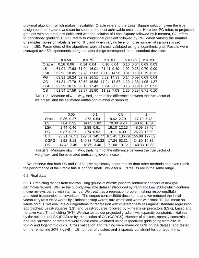
proximal algorithm, which makes it scalable. “Oracle” refers to the Least Square solution given the trueassignments of features and can be seen as the best achievable error rate. Here too, PG refers to projectedgradient with squared loss (initialized with the solution of Least Square followed by k-means), CG refersto conditional gradient, CGPG refers to conditional gradient followed by PG. When varying the numberof samples, noise on labels is set to σ = 0.5 and when varying level of noise σ number of samples is setto n = 150. Parameters of the algorithms were all cross-validated using a logarithmic grid. Results wereaveraged over 50 experiments and figures after the ± sign correspond to one standard deviation.
n = 50 n = 75 n = 100 n = 125 n = 150Oracle 0.16±0.06 0.14±0.04 0.10±0.04 0.10±0.04 0.09±0.03LS 61.94±17.63 51.94±16.01 21.41±9.40 1.02±0.18 0.70±0.09LSK 62.93±18.05 57.78±17.03 10.18±14.96 0.31±0.19 0.19±0.12PG 63.31±18.24 52.72±16.51 5.52±14.33 0.14±0.09 0.09±0.04CG 61.81±17.78 52.59±16.58 17.24±13.87 1.20±1.38 1.05±1.37CGPG 62.29±18.15 50.15±17.43 0.64±2.03 0.15±0.19 0.17±0.53OS 61.54±17.59 52.87±15.90 11.32±7.03 1.25±0.28 0.71±0.10
TABLE 2. Measure of ‖w∗ − w‖2, the l2 norm of the difference between the true vector ofweights w∗ and the estimated ones w along number of samples n.
σ = 0.05 σ = 0.1 σ = 0.5 σ = 1Oracle 0.86±0.27 1.72±0.54 8.62±2.70 17.19±5.43LS 7.04±0.92 14.05±1.82 70.39±9.20 140.41±18.20LSK 1.44±0.46 2.88±0.91 19.10±12.13 48.09±27.46PG 0.87±0.27 1.74±0.52 9.11±4.00 26.23±18.00CG 23.91±36.51 122.31±145.77 105.45±136.79 155.98±177.69CGPG 1.52±3.13 140.83±710.32 17.34±53.31 24.80±16.32OS 14.43±2.45 18.89±3.46 71.00±10.12 140.33±18.83
TABLE 3. Measure of ‖w∗ − w‖2, the l2 norm of the difference between the true vector ofweights w∗ and the estimated ones w along level of noise σ.
We observe that both PG and CGPG give significantly better results than other methods and even reachthe performance of the Oracle for n > d and for small σ, while for n ≤ d results are in the same range.
6.2. Real data.
6.2.1. Predicting ratings from reviews using groups of words. We perform “sentiment” analysis of newspa-per movie reviews. We use the publicly available dataset introduced by Pang and Lee [2005] which containsmovie reviews paired with star ratings. We treat it as a regression problem, taking responses for y in (0, 1)and word frequencies as covariates. The corpus contains n = 5006 documents and we reduced the initialvocabulary to d = 5623 words by eliminating stop words, rare words and words with small TF-IDF mean onwhole corpus. We evaluate our algorithms for regression with clustered features against standard regressionapproaches: Least-Squares (LS), and Least-Squares followed by k-means on predictors (LSK), Lasso andIterative Hard Thresholding (IHT). We also tested our projected gradient with sparsity constraint, initializedby the solution of LSK (PGS) or by the solution of CG (CGPGS). Number of clusters, sparsity constraintsand regularization parameters were 5-fold cross-validated using respectively grids going from 5 to 15, d/2to d/5 and logarithmic grids. Cross validation and training were made on 80% on the dataset and testedon the remaining 20% it gave Q = 15 number of clusters and d/2 sparsity constraint for our algorithms.
15

Results are reported in Table 4, figures after the ± sign correspond to one standard deviation when varyingthe training and test sets on 20 experiments.
All methods perform similarly except IHT and Lasso whose hypotheses does not seem appropriate for theproblem. Our approaches have the benefit to reduce dimensionality from 5623 to 15 and provide meaningfulcluster of words. The clusters with highest absolute weights are also the ones with smallest number ofwords, which confirms the intuition that only a few words are very discriminative. We illustrate this inTable 5, picking randomly words of the four clusters within which associated predictor weights vq havelargest magnitude.
LS LSK PG CG CGPG OS1.51±0.06 1.53±0.06 1.52±0.06 1.58±0.07 1.49±0.08 1.47±0.07
PGS CGPGS IHT Lasso1.53±0.06 1.49±0.07 2.19±0.12 3.77±0.17
TABLE 4. 100 × mean square errors for predicting movie ratings associated with reviews.
First and Second Cluster bad, awful,(negative) worst, boring, ridiculous,sizes 1 and 7 watchable, suppose, disgusting,Last and Before Last Cluster perfect,hilarious,fascinating,great(positive) wonderfully,perfectly,goodspirited,sizes 4 and 40 world, intelligent,wonderfully,unexpected,gem,recommendation,
excellent,rare,unique,marvelous,good-spirited,mature,send,delightful,funniest
TABLE 5. Clustering of words on movie reviews. We show clusters of words within whichassociated predictor weights vq have largest magnitude. First and second one are associatedto a negative coefficient and therefore bad feelings about movies, last and before last onesto a positive coefficient and good feelings about movies.
Acknowledgements. AA is at CNRS, at the Departement d’Informatique at Ecole Normale Superieure, 2rue Simone Iff, 75012 Paris, France. FB is at the Departement d’Informatique at Ecole Normale Superieureand INRIA, Sierra project-team, PSL Research University. The authors would like to acknowledge supportfrom a starting grant from the European Research Council (ERC project SIPA), an AMX fellowship, theMSR-Inria Joint Centre, as well as support from the chaire Economie des nouvelles donnees, the datascience joint research initiative with the fonds AXA pour la recherche and a gift from Societe GeneraleCross Asset Quantitative Research.
REFERENCES
Andreas Argyriou, Theodoros Evgeniou, and Massimiliano Pontil. Convex multi-task feature learning.Machine Learning, 73(3):243–272, 2008.
David Arthur and Sergei Vassilvitskii. k-means++: The advantages of careful seeding. In Proceedingsof the eighteenth annual ACM-SIAM symposium on Discrete algorithms, pages 1027–1035. Society forIndustrial and Applied Mathematics, 2007.
Francis Bach, Rodolphe Jenatton, Julien Mairal, and Guillaume Obozinski. Optimization with sparsity-inducing penalties. Found. Trends Mach. Learn., 4(1):1–106, January 2012. ISSN 1935-8237. doi:10.1561/2200000015.
Richard Bellman. A note on cluster analysis and dynamic programming. Mathematical Biosciences, 18(3):311–312, 1973.
16

David M. Blei, Andrew Y. Ng, and Michael I. Jordan. Latent dirichlet allocation. J. Mach. Learn. Res., 3:993–1022, March 2003. ISSN 1532-4435.
Thomas Blumensath and Mike E. Davies. Iterative hard thresholding for compressed sensing. Applied andComputational Harmonic Analysis, 27(3):265–274, 2009.
Howard D. Bondell and Brian J. Reich. Simultaneous regression shrinkage, variable selection, and super-vised clustering of predictors with oscar. Biometrics, 64(1):115–123, 2008.
Carlo Ciliberto, Youssef Mroueh, Tomaso Poggio, and Lorenzo Rosasco. Convex learning of multiple tasksand their structure. In Proceedings of the 32nd International Conference on Machine Learning, ICML2015, Lille, France, 6-11 July 2015, pages 1548–1557, 2015.
Inderjit S. Dhillon, Subramanyam Mallela, and Rahul Kumar. A divisive information theoretic featureclustering algorithm for text classification. The Journal of Machine Learning Research, 3:1265–1287,2003.
Ehsan Elhamifar and Rene Vidal. Sparse subspace clustering. In In CVPR, 2009.Marguerite Frank and Philip Wolfe. An algorithm for quadratic programming. Naval research logistics
quarterly, 3(1-2):95–110, 1956.Abner Guzman-Rivera, Pushmeet Kohli, Dhruv Batra, and Rob Rutenbar. Efficiently enforcing diversity
in multi-output structured prediction. In Proceedings of the Seventeenth International Conference onArtificial Intelligence and Statistics, pages 284–292, 2014.
Laurent Jacob, Jean-Philippe Vert, and Francis Bach. Clustered multi-task learning: A convex formulation.In Advances in Neural Information Processing Systems 21, pages 745–752. 2009.
Martin Jaggi. Revisiting frank-wolfe: Projection-free sparse convex optimization. In Proceedings of the30th International Conference on Machine Learning (ICML-13), pages 427–435, 2013.
Jung-Yi Jiang, Ren-Jia Liou, and Shie-Jue Lee. A fuzzy self-constructing feature clustering algorithm fortext classification. Knowledge and Data Engineering, IEEE Transactions on, 23(3):335–349, 2011.
Michael I. Jordan. Hierarchical mixtures of experts and the em algorithm. Neural Computation, 6:181–214,1994.
Bo Pang and Lillian Lee. Seeing stars: Exploiting class relationships for sentiment categorization withrespect to rating scales. In Proceedings of the 43rd Annual Meeting on Association for ComputationalLinguistics, pages 115–124. Association for Computational Linguistics, 2005.
N. Rao, B. Recht, and R. Nowak. Signal Recovery in Unions of Subspaces with Applications to CompressiveImaging. ArXiv e-prints, September 2012.
Robert Tibshirani, Michael Saunders, Saharon Rosset, Ji Zhu, and Keith Knight. Sparsity and smoothnessvia the fused lasso. Journal of the Royal Statistical Society: Series B (Statistical Methodology), 67(1):91–108, 2005.
Roman Vershynin. Introduction to the non-asymptotic analysis of random matrices. arXiv preprintarXiv:1011.3027, 2010.
Haizhou Wang and Mingzhou Song. Ckmeans. 1d. dp: optimal k-means clustering in one dimension bydynamic programming. The R Journal, 3(2):29–33, 2011.
Bin Zhang. Regression clustering. In ICDM, pages 451–. IEEE Computer Society, 2003. ISBN 0-7695-1978-4.
17

7. APPENDIX
7.1. Formulations for classification . We present here formulations of clustering either features or sampleswhen our task is to classify samples into K classes. For both settings we assume that n sample points aregiven, represented by the matrix X = (x1, ..., xn)T ∈ Rn×d and corresponding labels Y = (y1, . . . , yK) ∈0, 1n×K .
7.1.1. Clustering features for classification. Here we search K predictors W = (w1, . . . , wK), each ofthem having features clustered in Q groups G1, . . . ,GQ such that for any k, wjk = vqk if feature j is ingroup q. Partition of the features is shared by all predictors but each has different centroids represented inthe vector vk. Using an assignment matrix Z and the matrix of centroids V = (v1, . . . , vk), our problem cantherefore be written
minimize 1n
∑ni=1 loss
(yi, x
Ti W
)+ λ
2‖W‖2Fsubject to W = ZV, Z ∈ 0, 1d×Q, Z1 = 1
in variables W ∈ Rd×K , V ∈ RQ×K and Z. loss(yi, x
Ti W
)is a squared or logistic multiclass loss and
regularization can either be seen as a standard `2 regularization on the wk or a weighted regularization onthe centroids vk.
7.1.2. Clustering samples for classification. Here our objective is to form Q groups G1, . . . ,GQ of sam-ple points to maximize the within-group prediction performance. For classification, within each group Gq,samples are predicted using a common matrix of predictors V q = (vq1, . . . , v
qK). Our problem can be written
minimize1
n
∑
i∈Gq
loss(yi, x
Ti V
q)
+λ
2
Q∑
q=1
sq‖V q‖2F (17)
in the variables V = (V 1, . . . , V Q) ∈ Rd×K×Q and G = (G1, . . . ,GQ) such that G is a partition of the nsamples. loss
(yi, x
Ti W
)is a squared or logistic multiclass and λ
2
∑Qq=1 sq‖V q‖2F is a weighted regulariza-
tion. Using an assignment matrix Z ∈ 0, 1n×Q and auxiliary variables (W 1, . . . ,Wn) ∈ Rd×K×n suchthat W i = V q if i ∈ Gq, problem (17) can be rewritten
minimize 1n
∑ni=1 loss
(yi,W
iTxi
)+ λ
2
∑ni=1 ‖W i‖2F
subject to W T = ZV T , Z ∈ 0, 1n×Q, Z1 = 1,
in the variables W ∈ Rd×K×n, V ∈ Rd×K×Q and Z, where W = (Vec(W 1), . . . ,Vec(Wn)), V =(Vec(V 1), . . . ,Vec(V Q)) and for a matrix A, Vec(A) concatenates its columns into one vector.
Remark that in that case we must have K > Q otherwise we output more possible answers than classes(in that case the problem is ill-posed).
7.2. Clustered multitask . Our framework applies also to transfer learning by clustering similar tasks.Given a set of K supervised tasks like regression or binary classification, transfer learning aims at jointlysolving these tasks, hoping that each task can benefit from the information given by other tasks. For sim-plicity, we illustrate the case of multi-category classification, which can be extended to the general multitasksetting. When performing classification with one-versus-all majority vote, we train one binary classifier foreach class vs. all others. Using a regularizing penalty such as the squared `2 norm, the problem of multitasklearning can be cast as
minimize 1n
∑Kk=1
∑ni=1 loss(y
ki , w
Tk xi) + λ
∑Ki=1 ‖wk‖22. (18)
in the matrix variable W = (w1, . . . , wk) ∈ Rd×K of classifier vectors (one column per task). We writeLoss(y,X,W ) and R(W ) the first and second term of this problem. Various strategies are used to leveragethe information coming from related tasks, such as low rank Argyriou et al. [2008] or structured norm
18

penalties Ciliberto et al. [2015] on the matrix of classifiers W . Here we follow the clustered multitasksetting introduced in Jacob et al. [2009]. Namely we add a penalty Ω on the classifiers (w1, . . . , wK) whichenforce them to be clustered in Q groups G1, . . . ,GQ around centroids V = (v1, . . . , vQ) ∈ Rd×Q. Thispenalty can be decomposed in
• A measure of the norm of the barycenter of centers v = 1K
∑Qq=1 sqvq
Ωmean(V ) =λm2K||v||22
• A measure of the variance between clusters
Ωbetween(V ) =λb2
Q∑
q=1
sq||vq − v||22
• A measure of the variance within clusters
Ωwithin(W,V ) =λw2
Q∑
q=1
∑
i∈Gq
||wi − vq||22
The total penalty Ω(W,V ) = Ωmean(V ) + Ωbetween(V ) + Ωwithin(W,V ) is illustrated in Figure 2.
Ωwithin
ΩbetweenΩmean
0
FIGURE 2. Decomposed clustering penalty on K classes in the space of classifier vectors.
The clustered multitask learning problem can then be written using an assignment matrix Z and an auxil-iary variable W Denoting Π = I− 11T
K the centering matrix of the K classes, we develop each term of thepenalty,
Ωmean(V,Z) =λM2
Tr(V ZT (I−Π)ZV T ),
Ωbetween(V,Z) =λB2
Tr(V ZTΠZV T ),
Ωwithin(W,V,Z) =λW2||W − V ZT ||2F .
Using W = V ZT the total penalty can then be written
Ω(W, W ) =λM2
Tr(W (I−Π)W T ) +λB2
Tr(WΠW T ) +λW2||W − W ||2F ,
and the problem is
minimize Loss(y,X,W ) +R(W ) + Ω(W, W )
s.t. W T = ZV T , Z ∈ 0, 1K×Q, Z1 = 1,
in variables W ∈ Rd×K , W ∈ Rd×K , V ∈ Rd×Q and Z.19
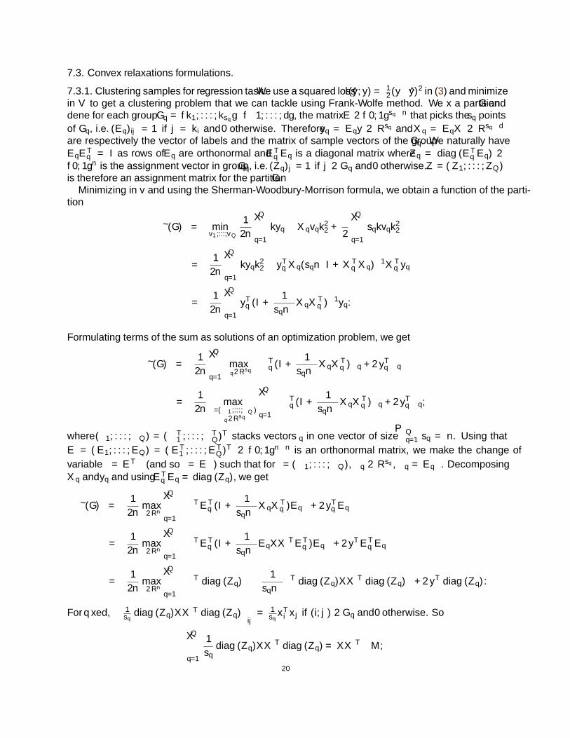
7.3. Convex relaxations formulations.
7.3.1. Clustering samples for regression task. We use a squared loss l(y, y) = 12(y−y)2 in (3) and minimize
in V to get a clustering problem that we can tackle using Frank-Wolfe method. We fix a partition G anddefine for each group Gq = k1, . . . , ksq ⊂ 1, . . . , d, the matrix E ∈ 0, 1sq×n that picks the sq pointsof Gq, i.e. (Eq)ij = 1 if j = ki and 0 otherwise. Therefore yq = Eqy ∈ Rsq and Xq = EqX ∈ Rsq×dare respectively the vector of labels and the matrix of sample vectors of the group Gq. We naturally haveEqE
Tq = I as rows of Eq are orthonormal and ETq Eq is a diagonal matrix where Zq = diag(ETq Eq) ∈
0, 1n is the assignment vector in group Gq, i.e. (Zq)j = 1 if j ∈ Gq and 0 otherwise. Z = (Z1, . . . , ZQ)is therefore an assignment matrix for the partition G.
Minimizing in v and using the Sherman-Woodbury-Morrison formula, we obtain a function of the parti-tion
ψ(G) = minv1,...,vQ
1
2n
Q∑
q=1
‖yq −Xqvq‖22 +λ
2
Q∑
q=1
sq‖vq‖22
=1
2n
Q∑
q=1
‖yq‖22 − yTq Xq(sqλnI +XTq Xq)
−1XTq yq
=1
2n
Q∑
q=1
yTq (I +1
sqλnXqX
Tq )−1yq.
Formulating terms of the sum as solutions of an optimization problem, we get
ψ(G) =1
2n
Q∑
q=1
maxαq∈Rsq
−αTq (I +1
sqλnXqX
Tq )αq + 2yTq αq
=1
2nmax
α=(α1;...;αQ)αq∈Rsq
Q∑
q=1
−αTq (I +1
sqλnXqX
Tq )αq + 2yTq αq,
where (α1; . . . ;αQ) = (αT1 , . . . , αTQ)T stacks vectors αq in one vector of size
∑Qq=1 sq = n. Using that
E = (E1; . . . ;EQ) = (ET1 , . . . , ETQ)T ∈ 0, 1n×n is an orthonormal matrix, we make the change of
variable β = ETα (and so α = Eβ) such that for α = (α1; . . . ;αQ), αq ∈ Rsq , αq = Eqβ. DecomposingXq and yq and using ETq Eq = diag(Zq), we get
ψ(G) =1
2nmaxβ∈Rn
Q∑
q=1
−βTETq (I +1
sqλnXqX
Tq )Eqβ + 2yTq Eqβ
=1
2nmaxβ∈Rn
Q∑
q=1
−βTETq (I +1
sqλnEqXX
TETq )Eqβ + 2yTETq Eqβ
=1
2nmaxβ∈Rn
Q∑
q=1
−βT diag(Zq)β −1
sqλnβT diag(Zq)XX
T diag(Zq)β + 2yT diag(Zq)β.
For q fixed,(
1sq
diag(Zq)XXT diag(Zq)
)ij
= 1sqxTi xj if (i, j) ∈ Gq and 0 otherwise. So
Q∑
q=1
1
sqdiag(Zq)XX
T diag(Zq) = XXT M,
20

where M = Z(ZTZ)−1ZT is the normalized equivalence matrix of the partition G and denotes theHadamard product. Using
∑Qq=1 diag(Zq) = I, we finally get a function of the equivalence matrix
ψ(M) =1
2nmaxβ∈Rn
−βT (I +1
λnXXT M)β + 2yTβ
=1
2nyT (I +
1
λnXXT M)−1y.
Its gradient is given by
∇ψ(M) = − 1
2λn2XXT
((I +
1
λnXXT M)−1yyT (I +
1
λnXXT M)−1
).
Algorithm 2 can be applied to minimize ψ. The linear oracle can indeed be computed with k-means usingthat the gradient is negative semi-definite. For a fixed Z, the linear predictors vq for each cluster of pointsare given by
vq = (nλsqI +XTq Xq)
−1XTq yq
= (nλsqI +XTETq EqX)−1XTETq Eqy
= (nλsqI +XT diag(Zq)X)−1XT diag(Zq)y.
7.3.2. Convex relaxations for classification. We observe that convex relaxations for classification derivefrom computations of the convex relaxations for regression by replacing vector of labels y by the corre-sponding matrix of labels Y .
INRIA - SIERRA PROJECT TEAM & D.I., UMR 8548,ECOLE NORMALE SUPERIEURE, PARIS, FRANCE.E-mail address: [email protected]
C.M.A.P., ECOLE POLYTECHNIQUE, UMR CNRS 7641E-mail address: [email protected]
CNRS & D.I., UMR 8548,ECOLE NORMALE SUPERIEURE, PARIS, FRANCE.E-mail address: [email protected]
INRIA - SIERRA PROJECT TEAM & D.I., UMR 8548,ECOLE NORMALE SUPERIEURE, PARIS, FRANCE.E-mail address: [email protected]
21