Learning Visual Scene Attributes

Vazheh Moussavivmoussav@cs.brown.edu

1 A Glance at Attribute-Centric Scene Representations

Take a look around you. How would you describe your surroundings to best give an idea of whateverything looks like to someone not there? Maybe you will give a category to the scene, say,‘bedroom’. You might try to list some of the objects around you, like ‘bed’, ‘lamp’, and ‘desk’. Orperhaps you’ll describe it with adjectives like ‘indoors’,‘cozy’, and ‘cluttered’. In computer vision,(or more specifically, in scene understanding), the most effective way to describe a visual scene isalso a major question.

Of the these three ways of describing a scene, (commonly referred to as categorization, scene pars-ing, and attribute-based representation respectively), categories have historically been the method ofchoice. In categorization, an image (scene) is allowed to fall into exactly one of an arbitrary numberof buckets. Attribute representations, however, are typically composed of several sets of bucketseach of which will have a value associated with that scene. For instance, a simple category-basedmodel would place an image in one of urban/rural/room, whereas a binary attribute-based modelwould have as attributes indoors and warm, each of which are marked as either present or not. Inlarger models, this leads to high dimensionality for attribute-based models, which has been a largedisincentive for its use. In addition, classifying a scene’s entire attribute set non-trivially falls un-dermulti-label learning, for which there exist very few learning algorithms in popular use. Lastly,there is scene parsing[5], which involves using object detectors, possibly in conjunction, to builddistributions over objects to define scenes.

Despite all this, attribute-centric models are becoming more popular. As seen in Figure 1, attribute-based representations give much more realistic partitionsof the space of visual scenes than cate-gories. We not only explicitly receive a fuller descriptionof the scene, but there is the added benefitof a potential way to measure a distance between two scenes that does not require storing means ofother images in the same category.

The authors of [2] further define visual attributes, introducing a dichotomy ofdiscriminativeandsemanticattributes. Discriminative attributes do not have any pre-defined meaning. Instead, theyare each built from trials where selected combinations of image classes (i.e. labels of categories andsemantic attributes) are used to accordingly place instances from the dataset in two partitions. For agiven partition, classifiers are trained on different lower-level (texture/color-based) features, and theresulting models that confidently and accurately discriminate among the selected classes are kept asthe discriminative attributes.

Semantic attributes, on the other hand, have an interpretable meaning (several examples of classesare shown in Figure 1). Semantic attribute classes may themselves be categorized differently bya general visual property relevant to modeling. As an example, let us consider spatial persistence.An attribute such as “rusty” is local: it is clear that it applies only to certain parts of a scene (therusty ones). Conversely, “open area” is a global attribute:its presence (according to our perception)can not be attributed to any specific part of a scene, and it applies entirely. Or, an attribute maybe spatially ambiguous: either it can exist in both local/global forms or we might not consciouslyknow (“driving” and “competing” being two examples). Clearly, modeling assumptions can affectthe understanding of local and global attributes differently.

1

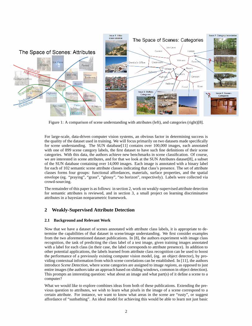
Figure 1: A comparison of scene understanding with attributes (left), and categories (right)[8].

For large-scale, data-driven computer vision systems, an obvious factor in determining success isthe quality of the dataset used in training. We will focus primarily on two datasets made specificallyfor scene understanding. The SUN database[11] contains over 100,000 images, each annotatedwith one of 899 scene category labels, the first dataset to have such fine definitions of their scenecategories. With this data, the authors achieve new benchmarks in scene classification. Of course,we are interested in scene attributes, and for that we look atthe SUN Attributes dataset[8], a subsetof the SUN database containing over 14,000 images. Each image is annotated with a binary labelfor each of 102 semantic scene attribute classes indicatingthat class’s presence. The set of attributeclasses forms four groups: functional affordances, materials, surface properties, and the spatialenvelope (eg. “praying”, “grass”, “glossy”, “no horizon”,respectively). Labels were collected viacrowd-sourcing.

The remainder of this paper is as follows: in section 2, work on weakly-supervised attribute detectionfor semantic attributes is reviewed, and in section 3, a small project on learning discriminativeattributes in a bayesian nonparametric framework.

2 Weakly-Supervised Attribute Detection

2.1 Background and Relevant Work

Now that we have a dataset of scenes annotated with attributeclass labels, it is appropriate to de-termine the capabilities of that dataset in scene/image understanding. We first consider examplesfrom the two aforementioned dataset publications. In [8], the authors experiment with image classrecognition, the task of predicting the class label of a testimage, given training images annotatedwith a label for each class (in their case, the label corresponds to attribute presence). In addition toother potential applications, the labels learned from attribute class recognition can be used to boostthe performance of a previously existing computer vision model, (eg. an object detector), by pro-viding contextual information from which scene correlations can be established. In [11], the authorsintroduceScene Detection, where scene categories are assigned to imageregions, as opposed to justentire images (the authors take an approach based on slidingwindows, common in object detection).This prompts an interesting question: what about an image and what part(s) of it define a scene to acomputer?

What we would like to explore combines ideas from both of these publications. Extending the pre-vious question to attributes, we wish to learn what pixels inthe image of a scene correspond to acertain attribute. For instance, we want to know what areas in the scene are “rusty”, or suggestaffordance of “sunbathing”. An ideal model for achieving this would be able to learn not just basic

2

features (color, texture, etc.) of an attribute, but high-level features that presumably humans alsoperceive and use to distinguish attributes (continuity/locality, size, shape, location, relation to sur-roundings, etc.). If successful, we could then construct a dictionary of visual definitions for an entireset of attributes.

Such a dictionary of semantic attributes has several possible applications. For instance, it couldincrease the range of output in artificial scene construction systems, by allowing users to apply at-tributes to areas of a scene, modifying them according to thelearned attribute definitions. Also, thereis the ability to query images by attribute, which would be a useful feature for image search engines.If the dictionary is particularly dense, one could imagine querying combinations of attributes tosolve other vision tasks. As an example, a ‘potted plant’ detector could exhaustively search overevery attribute combination known to correspond to potted plants, (‘leaves’, ‘indoors’, and ‘soil’being one example), and give a result based on the overlap of the attribute detections.

We now consider how to build such a model, by first consideringthe approaches in the examplesthat inspired our goal. In attribute recognition, we model not the appearance of an attribute itself butthe appearance of images in which the attribute is present. Nor do we model attribute location, con-tinuity, or size. For global scene attributes, it may be fairto assume that ignoring these distinctionshas a negligible effect in recognition; for local or space-ambiguous attributes, it is not. FollowingScene Detection and using a window-based approach is also undesirable. There is no attempt toisolate the presence of an attribute, because it only considers crops of the original image. Thus, weonly achieve approximations of attribute size, location, and continuity, and still do not model shapeat all.

Having ruled out other options, it would seem that in order toaccommodate modeling all of thedesired attribute characteristics mentioned before, we need to take an approach based on segmentingthe image. Most importantly, we would like for the segments to be relatively homogenous in theirdomains of description (a local attribute typically ceasesto apply only where there is a pronouncedchange in texture/color). Also, it is by using regions without any predefined structure that we canhope to model the shape of an attribute. Lastly, we have the capability of modeling size, location,and continuity of an attribute by interacting neighboring segments.

2.2 Problem Description and Approach

The problem we wish to solve falls under a category of machinelearning known asWeakly-Supervised Learning. It is supervised, in that our training data comes with classlabels (sceneattribute presence), but in a “weak” way, due to the fact thatthe labels lack part of the informa-tion we desire (per-pixel attribute detection). We will base much of our experimental work on asystem proposed for object detection[6]. (For clarity, we will refer to our application of the modelin terms of attributes instead.)

In the paper, the authors propose a very elegant to approach weakly-supervised learning in thecontext of computer vision. They take a segment-based approach, for many of the same reasonsmentioned earlier. Each individual segment is described bya featureF . They classify the segmentto an attribute based on the probability that the attribute is present in the containing image, whichthey nameR̃. They define an image asO if the attribute in question is present, andO if not, whichare the training labels that we are given. For a given segmentwith featureFi, they compute its scoreas:

R̃ (Fi) , P (O | Fi) =P (Fi | O)

P (Fi | O) + P(

Fi | O)

whereP (Fi | O) is the computed frequency ofFi over the training data. In other words, they useBayes’ Rule to obtain a posterior distribution among the setof segment feature values, setting theprior probabilitiesP (O) andP

(

O)

to be equal.

While this model is very clean and easy to understand, it doeshave some shortcomings. By con-sidering each segment individually, it is unable to consider attributes that are not bound by the seg-ments. Namely, for any global attribute (eg. electric light), the classifier would have to be convincedstrongly enough by each individual segment suggesting its presence (such as the area nearby a lampand the distinct soft shadows it creates). Ideally, a classifier would look around to piece togethersimilar nearby segments and use the greater collective presence to boost its score. In addition to the

3

Table 1: A simple visualization of the pipeline. An image is segmented (center), and each segmentis given a probability related to the presence of an attribute (right, rock/stone).

issues with spatial persistence and size, we are also unableto model shape and location with thissetup.

We now detail the pipeline used in our experiments, closely following the one described in [6].A visual description is provided in Table 1. The training data was the SUN Attributes dataset,which was broken into five equally-size ‘splits’ for the purpose of analyzing variance. We begin bysegmenting the image as the authors with a mean-shift based segmentation algorithm. The Edison[1]system was chosen not just for its free availability, but useand approval by the same authors in priorwork[7]. Parameters of the system were set to give larger andmore robust segments. Nearestneighbor smoothing was applied for the same reasons.

Region description was texture-based; a filter bank of two scales and 16 orientations was used tocompute responses. A texton vocabulary (100 words) is builtfrom clustering a random sample fromthe responses of a subset of the images in the SUN Attributes dataset. For every pixel in a segment,its filter bank response is then matched to a word from the texton vocabulary, accumulating in ahistogram. The k-means clustering and k-nearest neighborsmatching software was taken from theVLFEAT[9] website.

In our experiments, we tried two different attribute classifiers. First, the posterior-based approach aspreviously discussed. This is again accomplished by clustering the texton histograms of segmentsinto a feature vocabulary and matching to the words (vocabulary sizes of 50, 100, and 300 wereconsidered). The conditional frequenciesP (Fi | O) of the training set are then computed, leadingto the posterior probabilities necessary for classification. Another approach is to use a SupportVector Machine. The main benefit of using an SVM here is that because the texton histograms areused directly by the model, there is no loss of information due to quantization, which occurs in theposterior approach as a result of assigning the segment descriptors to feature words. On the otherhand, when using an SVM we no longer receive probabilities, but a classification score that is onlyable to make relative distinctions without setting an arbitrary threshold. (A linear SVM was used inthe experiments.)

2.3 Experiments

2.3.1 Results

Results from the posterior probability model were mixed, and general results are shown in Table 5(probabilities are displayed on a relative ‘jet’ colormap from blue to red). As previously hypoth-esized, the classifier performed much better for local attributes such as materials than global andambiguously-spatially persistent attributes. A comparison of the size of the feature vocabulary isshown in Table 3, and results are inconclusive, although there may be reason to believe that usingmore feature words could be beneficial (see the discussion section). Results among the differentsplits are shown in Table 2, and it can be seen that the data seems to give pretty consistent resultsamong them.

An SVM classifier was additionally built, primarily for reasons of comparison discussed in the pre-vious subsection. Table 6 shows visual results of the SVM classifier over multiple attributes and

4

Table 2: A comparison of the results for the rock/stone attribute among each of the five splits.Results are fairly consistent, as the same strips in the abbey are mapped to similar probabilities.

Table 3: A comparison of the posterior probability model using a vocabulary size of 50, 100, and300 words, respectively.

images, and we can see that the results are perhaps slightly worse. Specifically, results tendedto be oversmoothed. Analysis of the model output suggests again that the classifier is almost in-variably negative. The weights and bias variable varied significantly among attributes, The SVMslack parameter was varied in experiments to see possible effects it would have on the classifier(λ = 0.1, 1, 10), and an example is shown in Table 4.

2.3.2 Discussion

Perhaps the biggest issue with the results is the lack of absolute discriminatory power. As statedbefore, the colormaps of the result figures are all relative,which (at least in some cases) showthat the classifier does a good job of ordering segments in terms of their likelihood to indicate the

Table 4: A comparison of the svm model with different values for the slack parameter. Clearly, thereis very little difference in this range.

5

Table 5: Relative colormaps of the posterior model (100 words) for several images. Attributes fromleft to right: clouds, rugged scene, praying, glossy.

attribute in question. However, for the vast majority of results, the posterior probabilities are all in avery small range, meaning that the classifier is not learningthe attributes with enough confidence. Ahypothetical ROC curve of our classifier would have a sharp spike towards the top-left in one smallsegment, but stick close to the liney = x everywhere else, leading to an unsatisfactory area undercurve.

There is reason to believe that increasing the size of the feature vocabulary would be necessary inorder to boost the classifier’s discriminatory power. A likely explanation is that because of the largenumber of segments assigned to the same image attribute label (300-500 in most cases), there arenot enough distinct descriptors to vary along with the number of images in a given split, effectivelydividing the size of the training set by hundreds. While thisis all well and good, due to the resultantincrease in dimensionality, we would then need even more training images to accommodate the

6

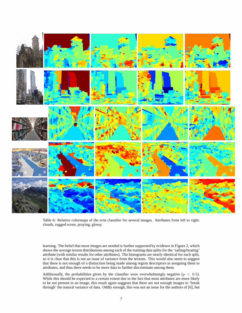
Table 6: Relative colormaps of the svm classifier for severalimages. Attributes from left to right:clouds, rugged scene, praying, glossy.

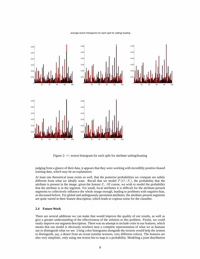
learning. The belief that more images are needed is further supported by evidence in Figure 2, whichshows the average texton distributions among each of the training data splits for the ‘sailing/boating’attribute (with similar results for other attributes). Thehistograms are nearly identical for each split,so it is clear that this is not an issue of variance from the textons. This would also seem to suggestthat there is not enough of a distinction being made among region descriptors in assigning them toattributes, and thus there needs to be more data to further discriminate among them.

Additionally, the probabilities given by the classifier were overwhelmingly negative (p < 0.5).While this should be expected to a certain extent due to the fact that most attributes are more likelyto be not present in an image, this result again suggests thatthere are not enough images to ‘breakthrough’ the natural variance of data. Oddly enough, this was not an issue for the authors of [6], but

7

20 40 60 80 1000

0.01

0.02

0.03

0.04

0.05

0.06

20 40 60 80 1000

0.01

0.02

0.03

0.04

0.05

0.06

20 40 60 80 1000

0.01

0.02

0.03

0.04

0.05

0.06

20 40 60 80 1000

0.01

0.02

0.03

0.04

0.05

0.06

average texton histograms for each split for sailing/ boating

20 40 60 80 1000

0.01

0.02

0.03

0.04

0.05

0.06

Figure 2: +/- texton histogram for each split for attribute sailing/boating

judging from a glance of their data, it appears that they wereworking with incredibly positive-biasedtraining data, which may be an explanation.

At least one theoretical issue exists as well, that the posterior probabilities we compute are subtlydifferent from what we ideally want. Recall that we modelP (O | Fi), the probability that theattribute is present in theimage, given the featureFi. Of course, we wish to model the probabilitythat the attribute is in the segment. For small, local attributes it is difficult for the attribute-presentsegments to collectively influence the whole image enough, leading to problems with negative bias,as discussed before. For global and ambiguously-persistent attributes, the attribute-present segmentsare quite varied in their feature description, which leads to copious noise for the classifier.

2.4 Future Work

There are several additions we can make that would improve the quality of our results, as well asgive a greater understanding of the effectiveness of the solution to this problem. Firstly, we couldeasily improve our segment description. There was no attempt to include color in our features, whichmeans that our model is obviously nowhere near a complete representation of what we as humansuse to distinguish what we see. Using color histograms alongside the textons would help the systemto distinguish, say, a desert from an ocean (similar textures, very different colors). The features arealso very simplistic, only using one texton bin to map to a probability. Modeling a joint distribution

8

over the features would allow for the classifier to learn and/or relationships among different featuretypes for a given attribute.

Next, our model does not consider using information from neighboring segments to determine like-lihoods of attribute presence in that segment. Using energy-based graphical models for weakly-supervised tasks has been previously explored, and this could be an important step in trying to learnspatial persistence of attribute classes, as proposed earlier. Lastly, our experiments clearly lack aquantitative analysis. Ideally, a labeling of each segmentwould be available, but even this would beseemingly too large a task to be crowd-sourced.

3 Learning Discriminative Attributes with Bayesian Nonparametrics

3.1 Introduction

We now turn our attention from semantic attributes to discriminative ones, as previously discussed.An interesting aspect not yet covered in much depth is developing a system for learning such at-tributes. Because we know so much less about discriminativeattributes than the semantic ones, wewill need to use a much more flexible approach. For this, we turn to bayesian nonparametrics. Usinga model known as the Indian Buffet Process[3], we consider a potentially infinite number of visualscene attributes to be learned in an unsupervised fashion. We first use the infinite factorial model ofbinary latent features with a linear-gaussian likelihood as described by [4]. We then move on to afully generativeNoisy-ORmodel for the IBP[10].

3.2 The Indian Buffet Process and Nonparametric Latent Feature Models

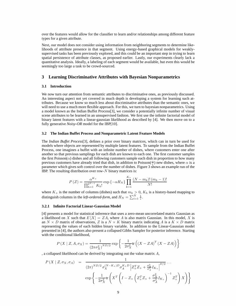
The Indian Buffet Process[3], defines a prior over binary matrices, which can in turn beused formodels where objects are represented by multiple latent features. To sample from the Indian BuffetProcess, one imagines a buffet with an infinite number of dishes, where customers enter one afteranother so that previous samplings for each dish are known toeach one. The first customer samplesthe first Poisson(α) dishes and all following customers sample each dish in proportion to how manyprevious customers have already tried that dish, in addition to Poisson(αi ) new dishes, whereα is aparameter which gives soft control over the number of dishes. Figure 3 shows an example run of theIBP. The resulting distribution over row-N binary matrices is:

P (Z) =αK+

∏2N−1

h=1 Kh!exp {−αHN}

K+∏

k=1

(N −mk)! (mk − 1)!

N !

whereK+ is the number of columns (dishes) such thatmk > 0, Kh is a history-based mapping todistinguish columns in theleft-ordered-form, andHN =

∑Ni=1

1i .

3.2.1 Infinite Factorial Linear-Gaussian Model

[4] presents a model for statistical inference that uses a zero-mean uncorrelated matrix Gaussian asa likelihood onX such thatE [X ] = ZA, whereA is also matrix Gaussian. In this model,X isanN × D matrix of observations,Z is aN × K binary matrix indicatingA is aK × D matrixrepresenting the values of each hidden binary variable. In addition to the Linear-Gaussian modelpresented in [4], the authors also present a collapsed GibbsSampler for posterior inference. Startingwith the conditional likelihood,

P (X | Z,A, σX) =1

(2πσ2X)

ND/2exp

{

−1

2σ2X

tr(

(X − ZA)T(X − ZA)

)

}

, a collapsed likelihood can be derived by integrating out the value matrixA,

P (X | Z, σX , σA) =1

(2π)ND/2σ(N−K+)DX σ

K+DA

∣

∣

∣ZT+Z+ +

σ2X

σ2A

IK+

∣

∣

∣

D/2. . .

exp

{

−1

2σ2X

tr

(

XT

(

I − Z+

(

ZT+Z+ +

σ2X

σ2A

IK+

)−1

ZT+

)

X

)}

9

Dish

Cus

tom

er

1 2 3 4 5 6 7 8 9101112131415161718192021222324

Figure 3: In the Indian Buffet Process, each customer (xi) samples dishes (zi) sequentially in pro-portion to how many previous customers have already tried each dish, with a fixed probability ofsampling a new dish.

whereZ+ andK+ respectively areZ andK with zero-sum columns removed. This, paired with anupdate for each elementzik of Z is updated to be “on” with a probability equal to the proportion ofother data points−i with featurek on, gives us a way to sample from the posterior distribution forZ, given the hyperparametersα, σX andσA.

3.2.2 Noisy-OR IBP

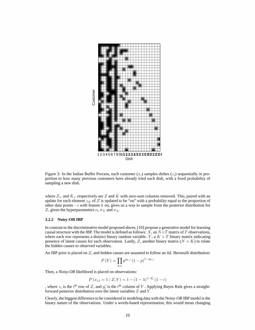
In contrast to the discriminative model proposed above, [10] propose a generative model for learningcausal structure with the IBP. The model is defined as follows: X , anN×T matrix ofT observations,where eachrow represents a distinct binary random variable.Y , aK × T binary matrix indicatingpresence of latent causes for each observation. Lastly,Z, another binary matrix (N ×K) to relatethe hidden causes to observed variables.

An IBP prior is placed onZ, and hidden causes are assumed to follow an iid. Bernoulli distribution:

P (Y ) =∏

k,t

pyk,t (1− p)1−yk,t

Then, aNoisy-ORlikelihood is placed on observations:

P (xi,t = 1 | Z, Y ) = 1− (1− λ)zi·y

′

t (1− ǫ)

, wherezi is theith row of Z, andy′t is thetth column ofY . Applying Bayes Rule gives a straight-forward posterior distribution over the latent variablesZ andY .

Clearly, the biggest difference to be considered in modeling data with the Noisy-OR IBP model is thebinary nature of the observations. Under a words-based representation, this would mean changing

10

Zα

A

X

σX

σA

α p

Z Y ǫ λ

X

Figure 4: (left) Graphical model for linear-Gaussian modelwith binary features (σA andσX are thestandard deviations forA andX , respectively, andα is the Poisson parameter for the basic IBP).(right) Graphical model for Noisy-OR IBP.ǫ is the the baseline probability thatxi,t = 1, λ is theprior probability of any cause affecting the observation, andp is the Bernoulli parameter for the iiddistribution over all hidden causesYk,t.

data from a direct histogram of quantized words to instead denote simply the “presence” of a word inan image, the implementation of which is non-trivial when considering issues of bias from samplingsize, among other factors.

[10] gives a Gibbs Sampler as well, although it is uncollapsed. The algorithm iterates through everylatent variable (1 . . .N ), within which it iterates through every cause (1 . . .K). First, eachzi,k issampled according to:

P (zi,k = a | X,Z−i,kY ) ∝ θa

k

(

1− θa

k

)(1−a) T∏

t=1

(

1− (1− λ)zi·y

′

t (1− ǫ))

|zi,k=a

, whereθk is the proportion of other data points−i with featurek “on”. Then, the number of newlatent features is sampled by

P(

Knewi | Xi,1:T , Zi,1:K+Knew

i, Y)

∝ P(

Xi,1:T | Zi,1:K+Knewi

, Y,Knewi

)

P (Knewi )

P(

Xi,1:T | Zi,1:K+Knewi

, Y,Knewi

)

=

T∏

t=1

P(

xi,t | Zi,1:K+Knewi

, Y,Knewi

)

P (xi,t = 1 | Znew, Y new,Knewi ) = 1− (1− ǫ) (1− λ)zi,1:K ·y1:K,t (1− λp)K

newi

, where the prior probability of newK values is Poisson(

αN

)

, as given by the IBP. Then each latentvariableyk,t is sampled from:

P (yk,t = a | Z,X, Y−k,t) ∝ pa (1− p)1−a

N∏

i=1

(

1− (1− λ)zi·y

′

t (1− ǫ))

|yi,k=a

3.3 Experiments

3.3.1 Data

To test the empirical validity of our model, we will run experiments on the SUN Attributes dataset,with a set of 102 manually-labeled visual attributes. The set of attributes is by no means visuallyexclusive, and there are significantly correlated attributes (eg. foliage and leaves). It is also nota ground truth, but instead a reasonable representation of visual scenes by human aesthetics, andwill be used as a means of assigning distances between images. In the following experiments,20 images which had been categorized as “park” and 20 categorized as “indoor theater” in theSUN database[11]. These categories were selected because of their inherent difference in visual

11

Figure 5: Example images used in experiments (top row: images of parks, bottom: images oftheaters)

appearance, and we intend to show that our model should be able to discriminate between the twowhile finding similarities in attributes within the same category. See Figure 5 for a few examples.

3.3.2 Results

The Linear-Gaussian Model had incredible difficulty mixingfor any vocabulary size larger than 20(thousands of iterations were necessary). This is possiblydue to the fact that integrating out thefactor loading matrixA is the source of too much variability and does not allow for large enoughsteps to be made, limiting mixing from taking place. In addition, further tweaking of the M-Hscheme may be necessary to avoid “killing” theσ parameters. The issues of these traits are supportedin Table 7 which shows average Hamming distances for the images used for experimentation. Whencompared to the aforementioned SUN Attributes database, the Linear-Gaussian model does not doas good of a job in discriminating between the two image categories, with a somewhat blurredinformation for smaller vocabularies. For larger vocabularies, the learned model seems to find alarger difference on average among park images than it does when comparing them to images oftheaters. Naturally, given the posterior mean ofA, an interesting experiment with this model wouldbe to attempt scene reconstruction. However, due to the great complexity of a natural scene, this isnearly impossible to do. In addition, a larger dataset, mostlikely to the order of millions, would beneeded.

Also unlike the Linear-Gaussian model, the Noisy-OR IBP model seemed to perform well at dis-criminating between the two image categories. Figure 6 displays a colormap of similarity for eachpossible pair of images. By measuring the average over all iterations of the mean equality amonghidden variables (Y ) for each image, it is easy to see that this learned model strongly distinguishesthe first 20 (park) images from the latter 20 (theatre). The reason thatY is used instead ofZ isbecause of the changed meaning of data points under this model (observations are considered to berepeats of individual variables, as opposed to instances ofsets of variables/features), soY representsthe latent space for theT = 40 images. It is also interesting to point out that, (roughly speaking),just as in the findings with the Linear-Gaussian model, theatre images were perceived as much closeramong each other than park images.

Hamming Distance SUN Attributes Learned Attributes (Linear-Gaussian)10 words 20 50 100 200

park 0.118 0.271 0.237 0.243 0.199 0.101theater 0.069 0.377 0.236 0.149 0.104 0.049

park-theater 0.155 0.383 0.272 0.210 0.166 0.081

Table 7: Comparison of average Hamming distances using the SUN Attributes 102 attributes vs.those learned by the Linear-Gaussian model with varying vocabulary sizes of quantized visualwords. Each row represents distance among park images, theater images, and cross-distances be-tween the two categories.

12

Latent Feature Overlap

5 10 15 20 25 30 35 40

5

10

15

20

25

30

35

40 0.2

0.3

0.4

0.5

0.6

0.7

0.8

0.9

1

Figure 6: Average equality of hidden causes (|Yi = Yj |), over run of Gibbs Sampler for Noisy-ORIBP. The first 20 data points are park images, the last 20 are ofindoor theaters.

3.3.3 Implementation Details

All code used to generate SIFT descriptors was provided by VLFEAT[9], which provides excellentinterfaces and documentation for the MATLAB code used for this project. The visual words werequantized using k-means, with a euclidean distance metric,as neither VLFEAT nor built-ins providea more appropriate histogram distance metric option (chi-squared, intersection, etc.).

For the Noisy-OR IBP model, the aforementioned “presence” of visual words was determined byplacing a threshold equal to the inverse of the number of quantized words, and choosing wordsthat were above this threshold as positive examples for observation data. This creates two flaws:first, that there is a somewhat arbitrary threshold, although this should not be an impactful issue,as natural variance among frequency of the words should cause most of the irrelevant words to bewashed out anyways, and choosing a large enough vocabulary will ensure this. Second, that thisintroduces dependencies among the hidden variables, because of the histogram representation of thevisual words. While this is certainly, true, one would hope that reduction to the simple binary caseand a small subset of quantized words helps mitigate this.

All code used to obtain these stated results are adapted fromFrank Wood’s academic website1.The inference code, along with its excellent (conference-submission-left-over) display code wasessentially unchanged itself. The collapsed sampler was implemented with few additional detailsnecessary from that derived in the original paper, following a prescribed Metropolis-Hastings stepfor resamplingα at each data point, or “customer”. In addition, Metropolis-Hastings steps were alsoprovided for the matrix Gaussian standard deviation parametersσA andσX .

The algorithmic decisions made for the Noisy-OR IBP model also was clear and made logical sense,but of course had more parameters to sample.p was initialized with a Beta(1,1), and afterwardsresampled with a Beta(|Yk,t = 1|,|Yk,t = 0|). α was initialized with a Gam(1,1) distribution, and re-

1http://www.stat.columbia.edu/ ˜ fwood/Code/index.html

13

sampled from Gam(1+K+, 11+HN

). Bothǫ andλ were initialized from a Uniform(0,1) distribution,and resampled using Metropolis-Hastings accept-reject procedures.

4 Acknowledgements

We would like to thank James Hays for his great research ideasand guidance as an advisor. Wewould also like to thank Genevieve Patterson for giving access to and experience with the SUNAttributes dataset.

14

References

[1] Christoudias, C., Georgescu, B., Meer, P.,Synergism in Low Level Vision, International Con-ference on Pattern Recognition, 2002.

[2] Farhadi, A., Endres, I., Hoiem, D., Forsyth, D.A.,Describing Objects by Their Attributes,CVPR 2009.

[3] Ghahramani, Z., Griffiths, T., Sollich, P.,Bayesian nonparametric latent feature models,Bayesian Statistics 8, 2007.

[4] Griffths, T. and Ghahramani, Z.,Infinite latent feature models and the Indian buffet process,Gatsby Institute for Computational Neuroscience, University College, London, 2006.

[5] Liu, C., Yuen, J., Torralba, A.,Nonparametric Scene Parsing via Label Transfer, IEEE Trans-actions on Pattern Analysis and Machine Intelligence, 2011.

[6] Pantofaru, C., Dorko, G., Schmid, C., Hebert, M.,A framework for learning to recognizeand segment object classes using weakly supervised training data, British Machine VisionConference (BMVC), 2007.

[7] Pantofaru, C., Hebert, M.,A Comparison of Image Segmentation Algorithms, 2005.

[8] Patterson, G., Hays, J.,SUN Attribute Database: Discovering, Annotating, and RecognizingScene Attributes, Proceeding of the 25th Conference on Computer Vision and Pattern Recog-nition (CVPR), 2012.

[9] Vedaldi, A., Fulkerson, B.,VLFeat: An Open and Portable Library of Computer Vision Algo-rithms, http://www.vlfeat.org/ , 2008.

[10] Wood, F., Griffiths, T., Ghahramani, Z.,A Non-Parametric Bayesian Method for InferringHidden Causes, Proceedings of the 22nd Conference on Uncertainty in Artificial Intelligence,2006.

[11] Xiao, J., Hays, J., Ehinger, K., Oliva, A., Torralba, A., SUN database: Large-scale scenerecognition from abbey to zoo, Computer Vision and Pattern Recognition (CVPR), 2010.

15