Learning Models for RobotNavigationHagit ShatkayPh.D. DissertationDepartment of Computer S ien eBrown UniversityProviden e, Rhode Island 02912CS-98-11De ember 1998

Learning Models for Robot NavigationbyHagit ShatkayB. S ., The Hebrew University of Jerusalem, 1989M. S ., The Hebrew University of Jerusalem, 1992

A dissertation submitted in partial ful�llment of therequirements for the Degree of Do tor of Philosophyin the Department of Computer S ien e at Brown UniversityProviden e, Rhode IslandMay 1999

Copyright 1997,1998,1999 by Hagit Shatkay

VitaName Hagit ShatkayBorn January 28, 1965 in Petah Tikva, IsraelEdu ation Brown University, Providen e, RIPh.D. in Computer S ien e, May 1999.The Hebrew University, Jerusalem, IsraelM.S . in Computer S ien e, Cum Laude, May 1992.The Hebrew University, Jerusalem, IsraelB.S . in Computer S ien e, Cum Laude, May 1989.Honors Brown University, Graduate Resear h Fellowship, 1997.The Hebrew University, Dean of the Fa ulty of Mathemat-i s and S ien es, List of A ademi Ex ellen e, 1988.The Hebrew University, Dean of the Fa ulty of Mathemat-i s and S ien es, A ademi Ex ellen e Award, 1986.Tea hing Experien e The Israeli Open University, Course Instru tor, 1988.The Israeli Open University, Course Dire tor, 1991.Military Servi e Lieutenant in the Israeli Defense For es, 1983-1985.i

ii

Abstra tHidden Markovmodels (hmms) and partially observable Markov de ision pro esses (pomdps)provide a useful tool for modeling dynami al systems. They are parti ularly useful for rep-resenting environments su h as road networks and oÆ e buildings, whi h are typi al forrobot navigation and planning. The work presented here des ribes a formal framework forin orporating readily available odometri information into both the models and the algo-rithm that learns them. By taking advantage of su h information, learning hmms/pomdps an be made better and require fewer iterations, while being robust in the fa e of dataredu tion. That is, the performan e of our algorithm does not signi� antly deteriorate asthe training sequen es provided to it be ome signi� antly shorter. Formal proofs for the onvergen e of the algorithm to a lo al maximum of the likelihood fun tion are provided.Experimental results, obtained from both simulated and real robot data, demonstrate thee�e tiveness of the approa h.iii

iv

To my parents, Sarah (Huber) and Adam Shatkay, in memoriam

v

vi

A knowledgmentsGetting a PhD is likely to be the end of my many years as a student. Throughout these years I wasfortunate to be surrounded by people whose wisdom and kindness helped make this time so pleasantand interesting. Unfortunately, I an not possibly list them all here, but I hope to thank at leastthose who have most prominently a�e ted the ourse I have taken so far.Several tea hers during elementary and high s hool in uen ed my hoi e of the s ienti� anda ademi dire tion. In parti ular, I thank Nira Efroni, Mr. Snook from the Lin oln primary s hoolin New Zealand, Pearl Friedman, Pessia Mi hael, Zvia Solomon and Tamar Ba hi.Sin e starting my a ademi studies, both in the Hebrew University of Jerusalem and at Brown,I had the privilege to learn from and work with some of the wisest and most extraordinary peoplein the omputer s ien e world.From the Hebrew University, I am espe ially grateful to Morde hai Tzipin, Saharon Shelah,Mi hael Rabin, Je� Rosens hein and Mori Rimon. The sound basis they have provided have servedme throughout my PhD work. Catriel Be'eri was myM.S . advisor, and introdu ed me to resear h inComputer S ien e. I am indebted to him for his non- ompromising demands for rigor and a ura y,and hope that some of his in uen e is evident in this thesis.At Brown, my deepest gratitude is extended to my advisor Leslie Pa k Kaelbling. Even priorto my be oming her student, she has readily shared her deep knowledge and unique insight, andprovided guidan e and en ouragement. Her enthusiasm, thoroughness and sheer enjoyment of thes ienti� work will remain with me, hopefully a�e ting the way I work and think.Tom Dean's kindness, support and good advi e during the early stages of my work, and histhoughtful omments as a thesis ommittee member were all extremely helpful. I am also mostgrateful to Sebastian Thrun from Carnegie Mellon University for being on my thesis ommittee, andfor his insightful omments on my thesis, enlightening dis ussions, and ontagious enthusiasm.John Hughes deserves many thanks for his help throughout the years, both with graphi s-orientedissues and with hard- ore mathemati s. I also thank Stanley Zdonik for being so up-beat anden ouraging during my �rst years in Brown, and for omplementing my theoreti al ba kground withhis \where's the beef" approa h. Eugene Charniak, Tom Doeppner, David Laidlaw, Philip Klein,Fran o Preparata, Roberto Tamassia and Eli Upfal have all been willing to answer my questionsand lend ma hine y les when needed. vii

From the amazing te hni al and administrative sta�, I espe ially thank Dorinda Multon andMax Salvas for putting up with more than their fair share of urgent and spe ial requests, JohnBazik, Kathy Kirman and Soren Spies for their helpfulness, and Susan (Platt) Hansen, JennetKirs henbaum, Dawn Ni holaus and Fran Palazzo for being so tolerant and a ommodating to allsorts of last-minute needs. I also thank Mary Andrade, Lori Agresti, Suzy Howe and Mary Killilea fortheir friendliness and assistan e. Trina Avery willingly answered numerous grammati al questions,and together with Leslie and Susan introdu ed me to the Providen e Singers and the Messiah singing.This is one of the most beautiful memories I have of my time in Brown, and I thank all three ofthem for this.A wonderful group of fellow graduate students has made my years in Brown so pleasurable.Lun hes with the \de women" | Beth Phalen, Nisha Thatte-Potter, Maria Loughlin and ShamsiMoussavi | and our ongoing reunions have all been joyful events. My �rst oÆ emate, Tony Cas-sandra, and his wife Ann Marie be ame good family friends. Tony has also been a partner for manyvaluable te hni al dis ussions. My urrent oÆ emates, Bill Smart, who sustains Ramona the robot,and Kee Eung Kim, have arried on this tradition both personally and professionally. Vaso Chatzi,has been a treasured friend all these years, as well as a valuable referen e sour e on many issues| from departmental news to geometry and algebra. This work would have literally looked verydi�erent without the relentless e�orts of Dimitris Mi hailidis as a Tex Mer . Manos Renieris, whojust repla ed Dimitris in this apa ity, has already performed several mira les as well. Friendshipaside, dis ussions with Luis Ortiz have greatly ontributed to my understanding of the em algo-rithm. I'm sure the sta� in \Montana" is going to miss our debates. Other people whose ompanyI enjoyed both so ially and professionally are Zori Atanassova, Sharon Caraballo, Jak Kirman, JimKurien, Sonia Lea h, Mi hael Littman, Andrew M Keith, Laurent Mi hel, Marian Nodine, BharathiSubramanian, Galina Shubina, Costas Bus h, Jos�e Casta~nos and Shieu-Hong Lin, as well as Ni olasMeuleau and Milos Hauskre ht.My family and friends in Israel have a ompanied me through the years. My sister Mi hal hasbeen an invaluable sour e of en ouragement and advi e, while my brother-in-law, Ira, has readilyserved as one of the better thesauri one ould hope for. Shula, my aunt, went out of her way tohelp, and without her assistan e after baby Ruth was born, it would have been very hard for meto resume my grad-s hool routine. Noga Amirav, David Mi haeli, Gadi Solotorevski and AvinoamKalma have kept our friendship going despite the distan e. I am thankful to them, as well as to therest of our family and friends in New England and in Israel.All this said, the one person to whom I am most grateful and obliged is my husband, YaronReshef. I annot thank him enough for his love, perseveran e, optimism, ex ellent ooking, and themany hours he has registered as a single parent throughout these years. Finally, my son, Eadoh,and daughter, Ruth, have been the most wonderful hildren in the world. Their heerful dispositionhelped put every experimental disaster and relu tant proof in perspe tive, and make the ombinationof motherhood and studentship so gratifying. viii

ContentsList of Tables xiiiList of Figures xv1 Introdu tion 11.1 HMMs and POMDP Models . . . . . . . . . . . . . . . . . . . . . . . . . . . 11.2 Models for Robot Navigation . . . . . . . . . . . . . . . . . . . . . . . . . . 21.3 Learning the Model . . . . . . . . . . . . . . . . . . . . . . . . . . . . . . . . 31.4 A New Approa h . . . . . . . . . . . . . . . . . . . . . . . . . . . . . . . . . 41.5 Thesis Outline . . . . . . . . . . . . . . . . . . . . . . . . . . . . . . . . . . 52 Approa hes to Learning Maps and Models 72.1 Learning Automata from Data . . . . . . . . . . . . . . . . . . . . . . . . . 72.1.1 Deterministi Automata . . . . . . . . . . . . . . . . . . . . . . . . . 102.1.2 Probabilisti Automata . . . . . . . . . . . . . . . . . . . . . . . . . 112.1.3 Models for Markov De ision Pro esses . . . . . . . . . . . . . . . . . 132.2 Learning Maps and Models for Robot Navigation . . . . . . . . . . . . . . . 142.2.1 Geometri Maps . . . . . . . . . . . . . . . . . . . . . . . . . . . . . 152.2.2 Topologi al Maps and Models . . . . . . . . . . . . . . . . . . . . . . 163 Models and Assumptions 193.1 HMMs { The Basi s . . . . . . . . . . . . . . . . . . . . . . . . . . . . . . . 193.2 Adding Odometry to Hidden Markov Models . . . . . . . . . . . . . . . . . 213.3 Extending POMDP Models . . . . . . . . . . . . . . . . . . . . . . . . . . . 23ix

4 Learning HMMs with Odometri Information 254.1 The Learning Problem . . . . . . . . . . . . . . . . . . . . . . . . . . . . . . 254.2 The Learning Algorithm . . . . . . . . . . . . . . . . . . . . . . . . . . . . . 274.2.1 Computing State-O upation Probabilities . . . . . . . . . . . . . . 284.2.2 Updating Model Parameters . . . . . . . . . . . . . . . . . . . . . . . 294.2.3 Stopping Criterion . . . . . . . . . . . . . . . . . . . . . . . . . . . . 334.2.4 Extending the Algorithm for Learning POMDPs . . . . . . . . . . . 344.3 Corre tness Proof of the Reestimation Formulae . . . . . . . . . . . . . . . 354.3.1 Transitions and Observations . . . . . . . . . . . . . . . . . . . . . . 364.3.2 Odometri Relations . . . . . . . . . . . . . . . . . . . . . . . . . . . 374.3.3 Constrained Odometri Relations . . . . . . . . . . . . . . . . . . . . 395 Dire tional Data and Distributions 435.1 Motivation . . . . . . . . . . . . . . . . . . . . . . . . . . . . . . . . . . . . 435.2 Statisti s of Dire tional Data . . . . . . . . . . . . . . . . . . . . . . . . . . 445.3 The von Mises Distribution . . . . . . . . . . . . . . . . . . . . . . . . . . . 465.4 Handling Angular Odometri Readings . . . . . . . . . . . . . . . . . . . . . 486 Choosing an Initial Model 516.1 K-Means-Based Initialization . . . . . . . . . . . . . . . . . . . . . . . . . . 536.2 Tag-Based Initialization . . . . . . . . . . . . . . . . . . . . . . . . . . . . . 557 Experiments within a Global Framework 617.1 Robot Domain . . . . . . . . . . . . . . . . . . . . . . . . . . . . . . . . . . 617.2 Evaluation Method . . . . . . . . . . . . . . . . . . . . . . . . . . . . . . . . 637.3 Results . . . . . . . . . . . . . . . . . . . . . . . . . . . . . . . . . . . . . . . 668 State-Relative Coordinate Systems 738.1 Motivation . . . . . . . . . . . . . . . . . . . . . . . . . . . . . . . . . . . . 738.2 Learning Odometri Relations with Relative Coordinates . . . . . . . . . . 758.2.1 Geometri al Consisten y in a Relative Framework . . . . . . . . . . 768.2.2 Initialization . . . . . . . . . . . . . . . . . . . . . . . . . . . . . . . 77x

8.2.3 Reestimation . . . . . . . . . . . . . . . . . . . . . . . . . . . . . . . 779 Experiments Using Relative Coordinates 799.1 Experimental Setting . . . . . . . . . . . . . . . . . . . . . . . . . . . . . . . 799.2 Results . . . . . . . . . . . . . . . . . . . . . . . . . . . . . . . . . . . . . . . 8110 Enfor ing Additivity 8710.1 Additivity within a Global Framework . . . . . . . . . . . . . . . . . . . . . 8810.2 Additivity within a Relative Framework . . . . . . . . . . . . . . . . . . . . 9110.3 Additive Heading Estimation . . . . . . . . . . . . . . . . . . . . . . . . . . 9210.3.1 Sele ting Fixed Entries . . . . . . . . . . . . . . . . . . . . . . . . . 9410.3.2 Proje tion onto an AÆne Spa e . . . . . . . . . . . . . . . . . . . . . 9511 Experiments Enfor ing Additivity 9911.1 Results within a Global Framework . . . . . . . . . . . . . . . . . . . . . . . 9911.2 Results within a Relative Framework . . . . . . . . . . . . . . . . . . . . . . 10311.3 Studying the E�e ts of Odometry and Additivity . . . . . . . . . . . . . . . 10512 Con lusions and Future Work 11312.1 Contributions . . . . . . . . . . . . . . . . . . . . . . . . . . . . . . . . . . . 11312.2 Future Work . . . . . . . . . . . . . . . . . . . . . . . . . . . . . . . . . . . 11412.3 Beyond Roboti s . . . . . . . . . . . . . . . . . . . . . . . . . . . . . . . . . 116A An Overview of the Odometri Learning Algorithm for HMMs 119B Di�erentiation Details 121B.1 Un onstrained Odometri Reestimation Formulae . . . . . . . . . . . . . . . 121B.2 Enfor ing Additivity within a Relative Framework . . . . . . . . . . . . . . 122Bibliography 125? Parts of this thesis have been previously published in the International Joint Confer-en e on Arti� ial Intelligen e, 1997, and in the International Conferen e on Ma hineLearning, 1998, by Hagit Shatkay and Leslie Pa k Kaelbling.xi

xii

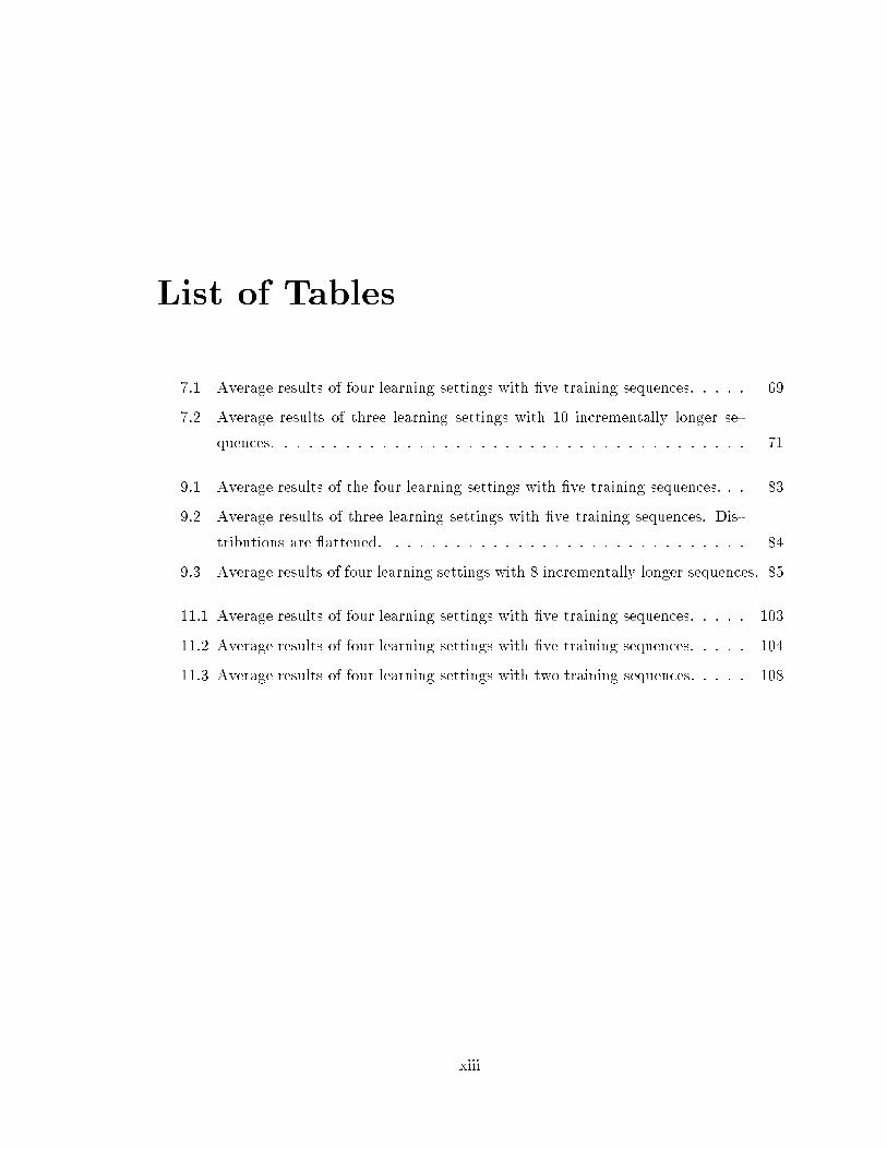
List of Tables7.1 Average results of four learning settings with �ve training sequen es. . . . . 697.2 Average results of three learning settings with 10 in rementally longer se-quen es. . . . . . . . . . . . . . . . . . . . . . . . . . . . . . . . . . . . . . . 719.1 Average results of the four learning settings with �ve training sequen es. . . 839.2 Average results of three learning settings with �ve training sequen es. Dis-tributions are attened. . . . . . . . . . . . . . . . . . . . . . . . . . . . . . 849.3 Average results of four learning settings with 8 in rementally longer sequen es. 8511.1 Average results of four learning settings with �ve training sequen es. . . . . 10311.2 Average results of four learning settings with �ve training sequen es. . . . . 10411.3 Average results of four learning settings with two training sequen es. . . . . 108xiii

xiv

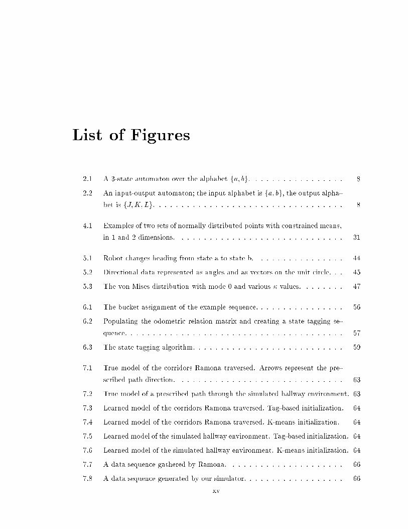
List of Figures2.1 A 3-state automaton over the alphabet fa; bg. . . . . . . . . . . . . . . . . 82.2 An input-output automaton; the input alphabet is fa; bg, the output alpha-bet is fJ;K; Lg. . . . . . . . . . . . . . . . . . . . . . . . . . . . . . . . . . 84.1 Examples of two sets of normally distributed points with onstrained means,in 1 and 2 dimensions. . . . . . . . . . . . . . . . . . . . . . . . . . . . . . 315.1 Robot hanges heading from state a to state b. . . . . . . . . . . . . . . . 445.2 Dire tional data represented as angles and as ve tors on the unit ir le. . . 455.3 The von Mises distribution with mode 0 and various � values. . . . . . . . 476.1 The bu ket assignment of the example sequen e. . . . . . . . . . . . . . . . 566.2 Populating the odometri relation matrix and reating a state tagging se-quen e. . . . . . . . . . . . . . . . . . . . . . . . . . . . . . . . . . . . . . . 576.3 The state tagging algorithm. . . . . . . . . . . . . . . . . . . . . . . . . . . 597.1 True model of the orridors Ramona traversed. Arrows represent the pre-s ribed path dire tion. . . . . . . . . . . . . . . . . . . . . . . . . . . . . . 637.2 True model of a pres ribed path through the simulated hallway environment. 637.3 Learned model of the orridors Ramona traversed. Tag-based initialization. 647.4 Learned model of the orridors Ramona traversed. K-means initialization. 647.5 Learned model of the simulated hallway environment. Tag-based initialization. 647.6 Learned model of the simulated hallway environment. K-means initialization. 647.7 A data sequen e gathered by Ramona. . . . . . . . . . . . . . . . . . . . . 667.8 A data sequen e generated by our simulator. . . . . . . . . . . . . . . . . . 66xv

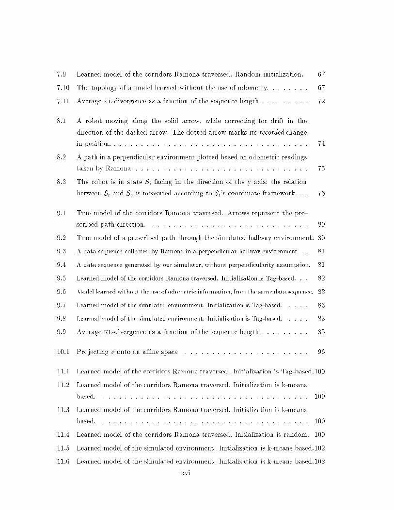
7.9 Learned model of the orridors Ramona traversed. Random initialization. 677.10 The topology of a model learned without the use of odometry. . . . . . . . 677.11 Average kl-divergen e as a fun tion of the sequen e length. . . . . . . . . 728.1 A robot moving along the solid arrow, while orre ting for drift in thedire tion of the dashed arrow. The dotted arrow marks its re orded hangein position. . . . . . . . . . . . . . . . . . . . . . . . . . . . . . . . . . . . . 748.2 A path in a perpendi ular environment plotted based on odometri readingstaken by Ramona. . . . . . . . . . . . . . . . . . . . . . . . . . . . . . . . . 758.3 The robot is in state Si fa ing in the dire tion of the y axis; the relationbetween Si and Sj is measured a ording to Si's oordinate framework. . . 769.1 True model of the orridors Ramona traversed. Arrows represent the pre-s ribed path dire tion. . . . . . . . . . . . . . . . . . . . . . . . . . . . . . 809.2 True model of a pres ribed path through the simulated hallway environment. 809.3 A data sequen e olle ted by Ramona in a perpendi ular hallway environment. . 819.4 A data sequen e generated by our simulator, without perpendi ularity assumption. 819.5 Learned model of the orridors Ramona traversed. Initialization is Tag-based. . . 829.6 Model learned without the use of odometri information, from the same data sequen e. 829.7 Learned model of the simulated environment. Initialization is Tag-based. . . . . 839.8 Learned model of the simulated environment. Initialization is Tag-based. . . . . 839.9 Average kl-divergen e as a fun tion of the sequen e length. . . . . . . . . 8510.1 Proje ting v onto an aÆne spa e . . . . . . . . . . . . . . . . . . . . . . . 9611.1 Learned model of the orridors Ramona traversed. Initialization is Tag-based.10011.2 Learned model of the orridors Ramona traversed. Initialization is k-meansbased. . . . . . . . . . . . . . . . . . . . . . . . . . . . . . . . . . . . . . . 10011.3 Learned model of the orridors Ramona traversed. Initialization is k-meansbased. . . . . . . . . . . . . . . . . . . . . . . . . . . . . . . . . . . . . . . 10011.4 Learned model of the orridors Ramona traversed. Initialization is random. 10011.5 Learned model of the simulated environment. Initialization is k-means based.10211.6 Learned model of the simulated environment. Initialization is k-means based.102xvi

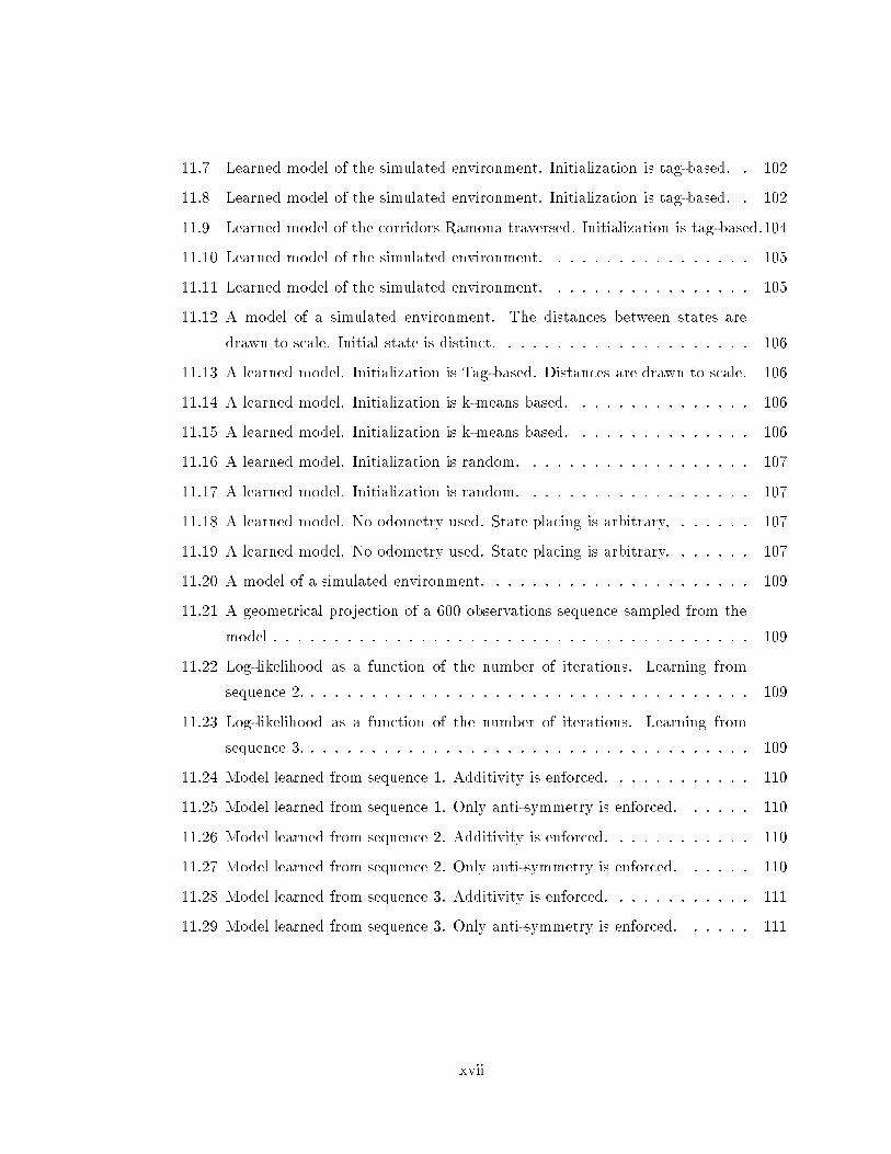
11.7 Learned model of the simulated environment. Initialization is tag-based. . 10211.8 Learned model of the simulated environment. Initialization is tag-based. . 10211.9 Learned model of the orridors Ramona traversed. Initialization is tag-based.10411.10 Learned model of the simulated environment. . . . . . . . . . . . . . . . . 10511.11 Learned model of the simulated environment. . . . . . . . . . . . . . . . . 10511.12 A model of a simulated environment. The distan es between states aredrawn to s ale. Initial state is distin t. . . . . . . . . . . . . . . . . . . . . 10611.13 A learned model. Initialization is Tag-based. Distan es are drawn to s ale. 10611.14 A learned model. Initialization is k-means based. . . . . . . . . . . . . . . 10611.15 A learned model. Initialization is k-means based. . . . . . . . . . . . . . . 10611.16 A learned model. Initialization is random. . . . . . . . . . . . . . . . . . . 10711.17 A learned model. Initialization is random. . . . . . . . . . . . . . . . . . . 10711.18 A learned model. No odometry used. State pla ing is arbitrary, . . . . . . 10711.19 A learned model. No odometry used. State pla ing is arbitrary. . . . . . . 10711.20 A model of a simulated environment. . . . . . . . . . . . . . . . . . . . . . 10911.21 A geometri al proje tion of a 600 observations sequen e sampled from themodel . . . . . . . . . . . . . . . . . . . . . . . . . . . . . . . . . . . . . . . 10911.22 Log-likelihood as a fun tion of the number of iterations. Learning fromsequen e 2. . . . . . . . . . . . . . . . . . . . . . . . . . . . . . . . . . . . . 10911.23 Log-likelihood as a fun tion of the number of iterations. Learning fromsequen e 3. . . . . . . . . . . . . . . . . . . . . . . . . . . . . . . . . . . . . 10911.24 Model learned from sequen e 1. Additivity is enfor ed. . . . . . . . . . . . 11011.25 Model learned from sequen e 1. Only anti-symmetry is enfor ed. . . . . . 11011.26 Model learned from sequen e 2. Additivity is enfor ed. . . . . . . . . . . . 11011.27 Model learned from sequen e 2. Only anti-symmetry is enfor ed. . . . . . 11011.28 Model learned from sequen e 3. Additivity is enfor ed. . . . . . . . . . . . 11111.29 Model learned from sequen e 3. Only anti-symmetry is enfor ed. . . . . . 111xvii

xviii

Chapter 1Introdu tionDynami al systems provide a formal mathemati al framework for des ribing many physi alphenomena. Possible states of a physi al system are represented as a set of verti es or nodes,and the dynami al aspe t of states hanging over time, as ar s or transitions. Sin e physi alphenomena are seldom either fully observable or ompletely predi table, it is also desirablefor dynami al systems to model the inherent un ertainty in observations and transitions.The work presented here is on erned with a quiring a parti ular family of models fordynami al systems, namely, Hidden Markov models.1.1 HMMs and POMDP ModelsHidden Markov models (hmms) represent a variety of nondeterministi dynami al systemsas abstra t probabilisti state-transition systems with dis rete states and observations. Thestates of the dynami al system are naturally mapped to the states of the model. The ob-servable aspe ts of ea h state in the dynami al system, whi h are often noisy and impre ise,are mapped to probability distributions or density fun tions over observations; ea h state inthe model has asso iated with it a distribution, or a probability density fun tion, over pos-sible observations. The un ertain dynami s of the modeled system is represented throughprobabilisti transitions between the model's states; ea h state is assigned a probabilitydistribution over the possible next states.Su h models are adequate for representing systems in whi h external entities exer iseno ontrol over the dynami s of the system, and the sto hasti behavior is ompletelyspe i�ed by the states, transitions and probabilities. They are widely used in a variety ofareas su h as natural language understanding [Cha93℄, spee h re ognition [Rab89, RJ93℄,1

2handwritten text analysis [CKZ94, BG95℄, and protein and DNA representation [Chu89,BCH+93, KBM+94℄.Hidden Markov models an be extended to model de ision pro esses in whi h ontrolis exer ised, by introdu ing a tions into the model. The extended models are known aspartially observable Markov de ision pro ess (pomdp) models. Like the basi hmm, a pomdpmodel has a set of states orresponding to the states of the modeled system. In addition, ea ha tion has asso iated with it a set of transition probability distributions { one distributionper state. The distribution models the probabilisti transition resulting from exe uting thea tion in the state. Similarly, ea h a tion has a set of observation probability distributions,one distribution per state, modeling the probabilisti observation whi h an be per eivedupon arrival at the state after exe uting the a tion.pomdp models are useful for modeling pro esses in whi h the out ome is un ertain andthe state is not fully observable. Su h pro esses arise in almost all aspe ts of life, from�nan ial investments to medi al de ision making. A variety of other appli ations is givenin work by Littman [Lit96℄ and Cassandra [Cas98℄.1.2 Models for Robot Navigationpomdp models have proven parti ularly useful as a basis for robot navigation in buildings,providing a sound method for lo alization and planning [SK95, NPB95, CKK96℄. Mostother approa hes to modeling environments for robot navigation [ME85, Asa91, LDWC91,TBF98℄ are on erned with obtaining a geometri al des ription of the environment, and are entered around �nding positions and lo ations in it, trying to determine exa tly where inthe environment the robot is. In ontrast, hmms and pomdp models are entered aroundthe on ept of state rather than that of lo ation.A state typi ally orresponds to a signi� ant landmark in the environment oupled withother important robot's attributes. Su h attributes may in lude the robot's orientation,its arm position, or its voltage level. This more general on ept, naturally aptures robotbehaviors and properties that do not ne essarily involve a hange in lo ation, su h as armmovement, pi king or dropping an obje t, amera positioning et . , thus providing a onsis-tent framework for planning and a ting in the environment. By being on erned with thetopology indu ed by signi� ant landmarks, rather than with the omplete geometry of thespa e, the models also tend to be more ompa t and support eÆ ient planning.Mu h previous work on planning using pomdp models has required that the model be

3provided, through manual spe i� ation. This is a tedious pro ess and it is often diÆ ultto obtain orre t probabilities. An ultimate goal is for an agent to be able to learn su hmodels automati ally, both for robustness and in order to ope with new and hangingenvironments.1.3 Learning the ModelFrom a theoreti al- omputational standpoint, hmms and pomdp models, an be viewed asprobabilisti �nite automata (pfa) and input/output pfa, respe tively. In the general ase,the onje ture is that learning su h models is hard, based on Abe and Warmuth's [AW92℄non-approximability results with respe t to probabilisti �nite automata, as des ribed inSe tion 2.1.2. Still, in pra ti e, the Baum-Wel h algorithm [Rab89℄ is frequently used tolearn hmms. Sin e pomdp models are a simple extension of hmms, they an, theoreti ally, belearned with a simple extension to the Baum-Wel h algorithm. However, in the general ase,without strong prior onstraint on the stru ture of the model, the Baum-Wel h algorithmdoes not perform very well: it is slow to onverge, requires a great deal of data, and is oftenstu k in lo al minima.Typi ally, appli ation domains in whi h hmm learning has proven su essful providesome bias whi h assists in the learning pro ess. For instan e, due to the temporal natureof the spee h pro ess, it an be modeled using a spe i� family of hmms, namely, left-to-right hmms [Rab89℄. In these models, transitions o ur in one dire tion only, and there areno y les other than ones aused by self-transitions. That is, the states an be indexed,su h that the probability of transitions from state i to state j, where j < i, is 0. This onstraint determines many of the model parameters, leaving fewer model parameters thata tually need to be learned, thus making the learning problem signi� antly simpler. Asimilar onstraint applies to handwritten text, as well as to biologi al stru tures su h asproteins or DNA, due to their sequential nature. Su h onstraints do not usually holdin the navigation domain, sin e in most real environments one an move ba k and forth,repeatedly visiting the same states via various distin t routes.Previous work, su h as Koenig and Simmons' [KS96b℄ used prior knowledge of theenvironment to bias the learning algorithm towards the orre t model. Using their approa h,a human provides a orre t but in omplete topologi al model of the environment, and theBaum-Wel h algorithm is used to �ll in the details. One of the entral goals of the workpresented here is to explore ways in whi h better models an be obtained, while using both

4less time and less data, without requiring a prior des ription of the learned environment.1.4 A New Approa hThe approa h taken in this work is based on utilizing a di�erent sour e of informationwhi h allows the Baum-Wel h algorithm to learn good topologi al models without the useof human-provided initial model. We propose to use readily available weak odometri in-formation to improve the results of the Baum-Wel h algorithm.Most robots are equipped with wheel en oders that enable an odometer to re ord the hange in the robot's position as it moves through the environment. This data is typi allyvery noisy and ina urate. The oors in the environment are rarely smooth, the wheelsof the robot are not always aligned and neither are the motors, a lot of the me hani s isimperfe t, resulting in slippage and drift. All these e�e ts a umulate, and if we were tomark the initial position of the robot, and try to estimate its urrent position based on along sequen e of odometri re ordings, we would �nd that our estimate is typi ally in orre t.That is, the raw re orded odometri information is not an e�e tive tool for determining theabsolute lo ation of the robot in the environment.The idea underlying our approa h is that this weak odometri information, despite itsnoise and ina ura y, still provides geometri al ues that an help to distinguish betweendi�erent states as well as to identify revisitation of the same state. Hen e, su h informationenhan es the ability to learn topologi almodels. However, the use of geometri al informationrequires areful treatment of geometri al onstraints and dire tional data.We demonstrate how the existing models and algorithms an be extended in order to takeadvantage of the noisy odometri data and the geometri al onstraints. The geometri alinformation is dire tly in orporated into the probabilisti topologi al framework, produ inga signi� ant improvement over the standard Baum-Wel h algorithm, without the need forhuman-provided model. Although there are still a number of intriguing problems thatneed to be addressed, our experiments prove that this is a promising dire tion in modela quisition for robot navigation.As a possible generalization to the problem of hmm a quisition, outside the s opeof roboti s, our approa h demonstrates the merit of using domain-spe i� onstraints toa hieve high utilization of the data, and restri t the learning pro ess, dire ting it towardsa quiring better models. We believe that this approa h an be put to use in other do-mains, su h as medi al de ision making and biologi al modeling. In the medi al domain,

5various onditions and symptoms ex lude ea h other, and temporal onstraints restri t thepossible transitions in the patient's state. In the mole ular biology domain, one an ex-ploit 3-dimensional geometri al onstraints over mole ular stru tures, whi h are likely tobe analogous to the onstraints arising when modeling environments for robot navigation.We expe t that by using these onstraints, the spa e of appropriate models whi h may �ta data set an be redu ed, and the model a quisition pro ess an be made more a urateand eÆ ient.1.5 Thesis OutlineThe rest of the thesis is organized as follows: Chapter 2 provides a survey of previous workin the area of learning maps and automata; Chapter 3 presents the formal framework forthis work; Chapter 4 des ribes the basi algorithm we have developed for using odometri information in the ontext of the Baum-Wel h algorithm; Chapter 5 dis usses spe ial issuesin handling dire tional data within a probabilisti framework; Chapter 6 presents methodsfor hoosing an initial model from whi h to start the algorithm, and introdu es a newmethod we have developed for this purpose; Chapter 8 des ribes ways to over ome theproblem of umulative rotational errors, whi h is another fa et of the problems aused bythe presen e of dire tional data and angular hanges; In Chapter 10 we provide a way forenfor ing omplete geometri al onsisten y in the topologi al model throughout the learningpro ess; Chapters 7, 9, and 11 present experimental results for ea h variant of our learningalgorithm. The experiments demonstrate that our algorithm indeed onverges to bettermodels with fewer iterations than the standard Baum-Wel h, and is robust in the fa e ofdata redu tion. In Chapter 12 we summarize the results and on lude the work, as well aslist several dire tions for future resear h.

6

Chapter 2Approa hes to Learning Maps andModelsThe work presented in this do ument lies in the interse tion between the theoreti al area oflearning omputational models | in parti ular learning automata from data sequen es |and the applied area of map a quisition for robot navigation. In the following we providea survey of results from both of these areas. The reinfor ement learning literature alsoaddresses some aspe ts of learning models for Markov de ision pro esses [Sut90, Thr92,Kae93℄. The latter an be viewed as a spe ial ase of learning probabilisti automata withfully observable states, and we brie y review related work from this domain in Se tion 2.1.3.2.1 Learning Automata from DataInformally speaking, an automaton onsists of a set of states, and a set of transitions whi hlead from one state to another. In the ontext of this work, the automaton states orrespondto the states of the modeled environments, and the transitions, to the state hanges dueto a tions performed in the environment. Ea h transition of the automaton is tagged by asymbol from an input alphabet, �, orresponding to the a tion or the input to the system,whi h aused the state transition. An example of an automaton with three states and inputalphabet fa; bg is shown in Figure 2.1.Classi al automata theory [HU79℄ distinguishes two types of spe ial states; a singleinitial state and a set of a epting states. If a sequen e of a tions starts from an initial stateand results in an a epting state, it is said that the automaton a epts the sequen e. For7

8a

a

32

1

a bbb

a

a

3

1

2

J

K L

a bbbFigure 2.1:A 3-state automaton over the al-phabet fa; bg. Figure 2.2:An input-output automaton; theinput alphabet is fa; bg, the output alphabet isfJ;K;Lg.instan e, in Figure 2.1, state 2 is depi ted as a double ir le, denoting an a epting state.If state 1 is assigned to be the initial state, the sequen es hai; hb ai and ha b ai; are alla epted by the automaton, while the sequen e ha bi is not.The basi stru ture des ribed above an be further extended to model the generationof output sequen es [HU79℄. This is done by de�ning an output alphabet � and assigningto ea h state a symbol in � that is emitted ea h time the state is rea hed. Su h extendedautomata are alled input-output automata. Figure 2.2 depi ts a 3-state automaton overthe input alphabet fa; bg and the output alphabet fJ;K; Lg. For instan e, if the inputsequen e is ha b ai and the initial state is 1, the generated output sequen e is hJ K J Ki.There are various possible kinds of un ertainty about the environment as well as theintera tion with it, whi h an be modeled through di�erent types of automata. First, statesin the environment an be either fully observable or partially observable. If the environmentis fully observable, one always knows its exa t state in the environment. When states areonly partially observable or hidden, one does not know its state with ertainty. In addition,the results of ea h a tion taken in the environment an be either fully determined or un er-tain. At any given state (be it observable or hidden), the exe ution of a fully deterministi a tion is guaranteed to lead to a single next state. The exe ution of an a tion with un er-tain results is not guaranteed to lead to a single next state and is modeled as a sto hasti transition fun tion. Given a pair onsisting of the urrent state and a tion, the transitionfun tion assigns to ea h state a probability of being rea hed through the a tion, from the urrent state. Based on these distin tions, we an partition automata into four groups:� Fully observable states, deterministi transitions� Fully observable states, sto hasti transitions� Hidden states, deterministi transitions� Hidden states, sto hasti transitions

9Automata with fully observable states an be viewed as input-output automata in whi hstates are distin tly labeled, the output alphabet onsists of state labels, and ea h stateemits its own label when visited. Automata with hidden states do not emit their statelabels, but might emit other output symbols (hen e the term partially observable).We an imagine an agent moving through an environment while re ording its per eivedobservations and a tions. The problem of learning an automaton, is informally des ribedas the problem of onstru ting an automaton that a epts the re orded sequen e of a tions,and emits the re orded sequen e of observations, if su h observations exist. In a settingwhere the automaton does not have a distin t a epting state, the learning problem issimilar, but merely requires that the learned automaton has a dire ted path through itsstates, orresponding to the re orded input (and/or output) sequen e.A ting in a fully observable and deterministi environment, orresponding to an au-tomaton of the �rst kind, we an re ord the origin state in whi h we start the exploration,as well as ea h subsequently visited state. In terms of de ision pro ess models, this an beviewed as a ting within the framework of deterministi Markov de ision pro esses [Put94℄.After visiting all the states (and exe uting all possible a tions - if we do have a hoi e ofa tion), we obtain a omplete model of the environment. That is, we deterministi ally knowhow to get from ea h state to all the other rea hable states. Hen e, learning a model ofsu h an environment is easy.The se ond kind of automata orresponds a sto hasti Markov de ision pro essmodel [Put94℄. Learning su h a model based on a sequen e of re orded visited statesand exe uted a tions, amounts to estimating transition probabilities under the exe uteda tions. It is a fairly simple task, under the assumption that the sequen e of re ordedstates is provided and we are not dealing with the problem of obtaining suÆ ient data forestimation purposes, and is dis ussed in Se tion 2.1.3.Obtaining models of the third and the fourth kinds, orrespond to the problems oflearning a deterministi and a probabilisti �nite automaton, respe tively. These problemsdo not have simple solutions in the general ase. The models and their respe tive learningproblems are dis ussed in detail in Se tions 2.1.1 and 2.1.2.It is also possible to have a fully deterministi environment in whi h an agent withimperfe t per eption re ords its a tions and observations. In this ase the agent may re ordthe wrong states, a tions or observations resulting in a noisy sequen e from whi h learningneeds to be done. In this ase, the learning pro edure needs to take into a ount that with

10some probability ea h re orded item may be wrong. The model learned is deterministi ,rather than sto hasti , but it might ontain errors with respe t to the true model, due tothe erroneous data from whi h it was learned. Some results under this s enario are alsodis ussed in Se tion 2.1.1.2.1.1 Deterministi AutomataA standard deterministi �nite automaton onsists of a �nite set of states Q, a �nite inputalphabet �, a transition fun tion Æ : Q � � ! Q, and a set F 2 Q of a epting states.The basi problem of learning �nite deterministi automata from given data an be roughlydes ribed as follows: Given two sets of positive and negative example strings, S and Trespe tively, over alphabet �, and a �xed number of states k, onstru t a minimal deter-ministi �nite automaton with no more than k states that a epts S and does not a ept T .This problem has been shown to be np- omplete [Gol78℄. Pitt and Warmuth [PW89℄ haveshown that even if we are not learning the minimal automaton of k states, but are willingto learn an automaton with a polynomial number of states f(k) with the same language,the problem is still np- omplete.Despite the hardness, positive results have been shown possible within various spe ialsettings. Angluin [Ang87℄ showed that if there is an ora le to answer membership queries(assuming a reset operator of the automaton to its initial state), and to provide ounterex-amples to onje tures about the automaton, there is a polynomial time learning algorithmfrom positive and negative examples. Rivest and S hapire [RS87b, RS87a℄ provide an ef-fe tive method for learning permutation automata, using distinguishing sequen es ( alled\tests") for disambiguating states. Their method is guaranteed to �nd an automaton thatwith high probability is the orre t one. In later work, [RS89℄, the authors use homingsequen es for the same purpose. They show that they an learn a orre t permutation au-tomaton in polynomial time assuming there is a \tea her" whi h provides ounterexamples,while a highly probable automaton an be learned even without the assumption of a tea her.All of the above work assumes deterministi , noise-free behavior of the learned automa-ton. As mentioned earlier, there are ases in whi h the training sequen e from whi h theautomaton is learned may be noisy. Basye, Dean and Kaelbling [BDK95℄ presented severalalgorithms that, with high probability, learn input-output deterministi automata whenvarious forms of noise are present in the training data. They show that when the transi-tions (a tions) are deterministi but output emissions (observations) are noisy, a polynomialtime algorithm exists, that learns a orre t deterministi model with high probability. The

11algorithm does not learn a distribution over the observations, but rather assumes that alikely observation exists for ea h state and this observation is the one learned. Thus thelearned model is ompletely deterministi rather than probabilisti . Similar results holdwhen the transitions are noisy and the observations are deterministi . (Again, the automa-ton learned is a deterministi one and does not model the transitions as probabilisti ). Forthe ase where both transitions and observations are noisy, a polynomial time algorithmfor learning a probably orre t deterministi automaton is given under strong assumptions,whi h in lude unique labeling of states.2.1.2 Probabilisti AutomataProbabilisti automata are ones in whi h a probability distribution governs the transitionsbetween states on any given input. In addition, in the ase of input-output automata, aprobability distribution is de�ned over the output emissions as well. The basi learningproblem in this ontext is to �nd an automaton that assigns the same distribution as thetrue one to data sequen es, from training data S generated by the true automaton. Anotherform of a learning problem is that of �nding a probabilisti automaton � that assigns themaximum likelihood to the training data S, that is, an automaton that maximizes Pr(Sj�).Abe and Warmuth [AW92℄ show that �nding a probabilisti automaton with 2 states,even when small error with respe t to the true model is allowed with some probability (theProbably Approximately Corre t learning model), annot be done in polynomial time witha polynomial number of examples, unless np = rp. They also show the equivalen e of theproblem of learning an automaton in the pa sense to that of approximating the maximumlikelihood automaton. This means that approximating a solution to any of the two learningproblems stated above, for a probabilisti automaton, is equivalently hard. From theirwork arises a broader onje ture, whi h has not yet been proven, that the general problemof learning probabilisti automata with any number of states, even under the pa learningmodel, is hard. A similar broadly a epted onje ture stemming from the same work is thatlearning hidden Markov models (the kind of probabilisti automata formally introdu ed inSe tion 3.1) is hard even in the pa sense.Two ways of addressing this hardness are presented in the rest of this se tion. One usesrestri tions on the lass of probabilisti models learned, and the other learns an unrestri tedhidden Markov model with good pra ti al results but with no pa guarantees on the qualityof the result.

12 Restri ting the Learning Problem: In their above mentioned paper, Abe and War-muth suggest that an interesting open problem is to �nd sub lasses of probabilisti automatathat are both pra ti ally useful and polynomially pa learnable.Work by Ron et al. [RST94, RST95, RST98℄ pursues su h an approa h. The authorspresent two lasses of probabilisti automata that are useful in the area of natural languageunderstanding, in parti ular for ursive hand writing re ognition, spee h re ognition andprinted text analysis. One su h lass onsists of a y li probabilisti �nite automata, andthe other of probabilisti �nite suÆx automata. Both of these lasses an be learned inpolynomial time (in all the parameters) within the pa framework.Learning with Restri ted Guarantees: Another approa h, the one predominantlytaken in this work, is to learn a model for the data from the omplete unrestri ted lass ofhidden Markov models. Only weak guarantees exist about the goodness of the model, butthe learning pro edure may be dire ted to obtain pra ti ally good results.This approa h is based on guessing an automaton (model), and using an iterative pro- edure to make the automaton �t the training data better. One algorithm ommonly usedfor this purpose is the Baum-Wel h algorithm [BE67, BS68, BPS+70℄, whi h is presentedin detail by Rabiner [Rab89℄. The iterative updates of the model are based on gatheringsuÆ ient statisti s from the data given the urrent automaton, and the update pro e-dure is guaranteed to onverge to a model that lo ally maximizes the likelihood fun tionPr(datajmodel). Sin e the maximum is lo al, the model might not be lose enough to theautomaton by whi h the data was generated, and a hallenging problem is to �nd ways tofor e the algorithm into onverging to higher maxima, or at least to make it onverge faster,fa ilitating multiple guesses of initial models, thus raising the probability of onverging tohigher maxima. Su h an approa h is the one taken in this work.Throughout this work we assume that the number of states in the model we are learningis given as input. This is not a very strong assumption, sin e there exist methods for learningthe number of states. A natural generalization of the algorithm presented here is to applysu h methods to dire tly learn the number of states from the data. Obviously, without anybound on the number of states, one an designate a state for ea h data point in the inputsequen e, thus perfe tly �tting the data. Su h an approa h is a trivial example of over�tting;the model indeed �ts the data well but is not general enough for modeling other dataobtained from the same modeled environment. Regularization methods are used in orderto avoid over�tting, dire ting the learning pro ess towards models that �t both the urrenttraining data as well as yet-unseen data. One su h te hnique is ross-validation [Sto74,

13Sha93, ET93℄. Its basi idea is to use only parts of the available data to learn models ofvarying number of states, while saving some of the data for testing purposes. On e severalmodels are learned, the likelihood (or some other measure of goodness) that they assign tothe part of the data not used for learning is ompared. The number of states for the modelthat has the highest measure of goodness, is taken to be the orre t number of states, andis �xed. A �nal model is then obtained by learning from the omplete data under the �xednumber of states. Other regularization methods su h as the minimum des ription lengthprin ipal for de iding on the number of states and other model parameters, are dis ussedin Vapnik's book [Vap95℄. Another similar riterion suggested by Akaike is des ribed in abook by Sakamoto et al. [SIK86℄. In Se tion 6.2 we suggest another possible heuristi forestimating the number of states as part of an initialization algorithm.2.1.3 Models for Markov De ision Pro essesMu h of the work on reinfor ement learning [Kae93, Sut90, Thr92, BBS95, MB98℄ is on- erned with a ting optimally within the ontext of fully observable Markov de ision pro- esses. The Markov model onsists of states and a tions that transition an agent from onestate to the other, where every su h transition has asso iated with it a reward. The goalof the agent is to optimize its reward. The transitions between states are usually sto has-ti , and the agent does not always know either the probability distribution governing thetransition or the reward asso iated with ea h state-a tion pair. In su h ases, where theparameters are unknown to the agent, it tries to obtain knowledge about them via explo-ration. The main idea behind exploration is that by taking a tions at ea h state, the agentobtains ounts of the number of times it ended up in every state. It uses the ounts to al- ulate suÆ ient statisti s and estimate the transition probabilities whi h it does not knowa priori. Given a sequen e of states re orded during exploration, learning the model is astraightforward statisti al estimation problem [Bil59℄. The more involved issue is that ofde iding on strategies to explore the environment in order to obtain the data [Mar67℄.This form of model learning is di�erent from the problem we are addressing, sin e in thehmm and pomdp ase the state itself is hidden and one an not dire tly obtain transition ounts between states and al ulate statisti s. Another aspe t of the learning in a partiallyobservable environment is that of learning the observation distribution asso iated with ea hstate, as des ribed in Chapter 3. This aspe t does not exist in the fully observable ase.

142.2 Learning Maps and Models for Robot NavigationThe other area whi h losely relates to the work presented here is that of modeling envi-ronments for robot navigation. A distin tion is usually made between two prin ipal kindsof maps: geometri and topologi al. Geometri maps des ribe the environment as a olle -tion of obje ts or o upied positions in spa e, and the geometri relationships among them.The topologi al framework is less on erned with the geometry, and models the world as a olle tion of states and their onne tivity, that is, whi h states are rea hable from ea h ofthe other states and what a tions lead from one state to the next.We draw an additional distin tion, between world- entri 1 maps that provide an \ob-je tive" des ription of the environment independent of the agent using the map, and robot- entri models whi h apture the intera tion of a parti ular \subje tive" agent with theenvironment. When learning a map, the learning agent needs to take into a ount its ownnoisy sensors and a tuators and try to obtain an obje tively orre t map that other agents ould use as well. Similarly, other agents using the map need to ompensate for their ownlimitations in order to assess their position a ording to the map. When learning a modelthat aptures intera tion the agent a quiring the model is the one who is also using it.Hen e, the noisy sensors and a tuators spe i� to the agent are re e ted in the model. Adi�erent model is likely to be needed by di�erent agents. Most of the related work des ribedbelow, espe ially within the geometri al framework, is entered around learning obje tivemaps of the world rather than agent-spe i� models. We shall point out in this survey thework that is on erned with the latter kind of models.Our work fo uses on a quiring purely topologi al models, and is less on erned withlearning geometri al relationships between lo ations or obje ts, or obje tive maps, althoughgeometri al relationships do serve as an aid in our a quisition pro ess. The on ept of astate used in this topologi al framework is more general than the on ept of a geometri allo ation, sin e a state an in lude information su h as the battery level, the arm positionet . Su h information, whi h is of great importan e for planning, is non-geometri al innature and therefore an not be readily aptured in a purely geometri al framework. Thefollowing provide a survey of both work done within the geometri al framework and withinthe topologi al framework as well as ombinations of the two approa hes.1I thank Sebastian Thrun for the terminology.

152.2.1 Geometri MapsGeometri maps provide a des ription of the environment in terms of the obje ts pla edin it and their positions. For example, grid-based maps are an instan e of the geometri approa h. In a grid-based map, the environment is modeled as a grid (an array), whereea h position in the grid an be either va ant or o upied by some obje t (binary valuespla ed in the array). This approa h an be further re�ned to re e t un ertainty about theworld, by having grid ells ontain o upan y probabilities rather than just binary values.A lot of work has been done on learning su h grid-based maps for robot navigation, throughthe use of sonar readings and their interpretation, by Movare and Elfes and others [ME85,Mor88, Elf89, Asa91℄.An underlying assumption when learning su h maps is that the robot an tell where it ison the grid when it obtains a sonar reading indi ating an obje t, and therefore an pla e theobje t orre tly on the grid. A similar lo alization assumption underlies other geometri mapping te hniques [LDWC91, SSC91, TGF+98℄, even when an expli it grid is not partof the model. This assumption an be hard to satisfy. Leonard and Cox [LDWC91℄ andSmith et al. [SSC91℄ address this issue through the use of geometri al bea ons to estimatethe lo ation of the robot. A probability distribution is used to model the robot's possible urrent lo ation, based on observations olle ted up to the urrent point.Re ent work by Thrun et al. [TBF98℄, uses a similar probabilisti approa h for obtaininggrid-based maps. This work is re�ned [TGF+98℄ to �rst learn the lo ation of signi� antlandmarks in the environment and then �ll in the details of the omplete geometri al grid,based on laser range s ans. The latter work extends the approa h of Smith et al. , by usingobservations obtained both before and after a lo ation has been visited, in order to derive aprobability distribution over possible lo ations. To a hieve this, the authors use a forward-ba kward pro edure similar to the one used in the Baum-Wel h algorithm [Rab89℄, (seeChapter 4 of this work), in order to determine possible lo ations from observed data. Theapproa h resembles ours both in the use of the forward-ba kward estimation pro edure, andin its probabilisti basis, aiming at obtaining a maximum likelihood map of the environment.It still signi� antly di�ers from ours both in its initial assumptions and in its �nal results.The data assumed to be provided to the learner in ludes both the motion model and theper eptual model of the robot. These onsist of transition and observation probabilitieswithin the grid. Both of these omponents are learnt by our algorithm, although not ina grid ontext but in a topologi al, oarser-grained, framework. The end result of theiralgorithm is a probabilisti grid-based map, while ours is a probabilisti topologi al model.

16 In addition to being on erned only with lo ations, rather than with the ri her notionof state, a fundamental drawba k of geometri al maps is their �ne granularity and higha ura y. Geometri al maps, parti ularly grid-based ones, tend to give an a urate anddetailed pi ture of the environment. In ases where it is ne essary for a robot to knowits exa t lo ation in terms of metri oordinates, metri maps are indeed the best hoi e.However, many planning tasks do not require su h �ne granularity or a urate measures,and are better fa ilitated through a more abstra t representation of the world. For example,if a robot needs to deliver a bagel from oÆ e a to oÆ e b, all it needs to have is a mapdepi ting the relative lo ation of a with respe t to b, the passageways between the twooÆ es, and perhaps a few other landmarks to help it orient itself if it gets lost. If it has areasonably well-operating low-level obsta le avoidan e me hanism to help it bypass owerpots and hairs that it might en ounter on its way, su h obje ts do not need to be part ofthe environment map. Just as a driver traveling between ities needs to know neither itslongitude and latitude oordinates on the globe, nor the lo ation of the spe i� houses alongthe way, the robot does not need to know its exa t lo ation within the building nor theexa t lo ation of various items in the environment, in order to get from one point to another.Hen e, the e�ort of obtaining su h detailed maps is not usually justi�ed. In addition themaps an be very large, whi h makes planning | even though planning is polynomial inthe size of the map | be ineÆ ient.2.2.2 Topologi al Maps and ModelsAn alternative to the detailed geometri maps are the more abstra t topologi al maps.Su h maps spe ify the topology of important landmarks and situations (states), and routesor transitions (ar s) between them. They are less on erned with the physi al lo ation oflandmarks, and more with topologi al relationships between situations. Typi ally, they areless omplex and support mu h more eÆ ient planning than metri maps. Topologi al mapsare built on lower-level abstra tions that allow the robot to move along ar s (perhaps bywall- or road-following), to re ognize properties of lo ations, and to distinguish signi� antlo ations as states; they are exible in allowing a more general notion of state, possiblyin luding information about the non-geometri al aspe ts of the robot's situation.There are two typi al strategies for deriving topologi al maps: one is to learn the topo-logi al map dire tly; the other is to �rst learn a geometri map, then to derive a topologi almodel from it through some pro ess of analysis.A ni e example of the se ond approa h is provided by Thrun and B�u ken [TB96a,

17TB96b, Thr99℄, who use o upan y-grid te hniques to build the initial map. This strategyis appropriate when the primary ues for de omposition and abstra tion of the map aregeometri . However, in many ases, the nodes of a topologi al map are de�ned in terms ofother sensory data (e.g. labels on a door or whether or not the robot is holding a bagel).Learning a geometri map �rst also relies on the odometri abilities of a robot; if they areweak and the spa e is large, it is very diÆ ult to derive a onsistent map.In ontrast, our work on entrates on learning a topologi al model dire tly, assumingthat abstra tion of the robot's per eption and a tion abilities has already been done. Su habstra tions were manually en oded into the lower level of our robot navigational software,as des ribed in Chapter 7. Work by Pier e and Kuipers [PK97℄ dis usses an automati method for extra ting abstra t states and features from raw per eptual information.Kuipers and Byun [KB91℄ provide a strategy for learning deterministi topologi al maps.It works well in domains in whi h most of the noise in the robot's per eption and a tion isabstra ted away, learning from single visits to nodes and traversals of ar s. An underlyingassumption for this strategy is that the urrent state an be reliably identi�ed based onlo al information, or based on distan e traversed from the previous well-identi�ed state.It is unable to handle situations in whi h long sequen es of a tions and observations arene essary to disambiguate the robot's state.Engelson and M Dermott [EM92℄ learn \diktiometri " maps (topologi al maps withmetri relations between nodes) from experien e. The un ertainty model they use is interval-based rather than probabilisti , and the learned representation is deterministi . Ad ho routines handle problems resulting from failures of the un ertainty representation.We prefer to learn a ombined model of the world and the robot's intera tion with theworld; this allows robust planning that takes into a ount likelihood of error in sensing anda tion. The work most losely related to ours is by Koenig and Simmons [KS96b, KS96a℄,who learn pomdp models (sto hasti topologi al models) of a robot hallway environment.They also re ognize the diÆ ulty of learning a good model without initial information;they solve the problem by using a human-provided topologi al map, together with further onstraints on the stru ture of the model. A modi�ed version of the Baum-Wel h algo-rithm learns the parameters of the model. They also developed an in remental version ofBaum-Wel h that an be used on-line. Their models ontain very weak metri information,representing hallways as hains of one-meter segments and allowing the learning algorithmto sele t the most probable hain length. This method is e�e tive, but results in large mod-els with size proportional to the hallways length, and strongly depends on the provision of

18a good initial model.The rest of the work des ribes our approa h to learning topologi al models. We showthat by using weak odometri information dire tly, we an avoid the use of human-provideda priori models and still learn sto hasti maps eÆ iently and e�e tively.

Chapter 3Models and AssumptionsThis hapter des ribes the basi s of the formal framework for our work. It starts by in-trodu ing the lassi hidden Markov model. The model is then extended to a ommodatenoisy odometri information in its simplest form, ignoring information about the robot'sheading and orientation. In hapters 5 and 8, the model is further extended and re�ned toa ommodate heading information and address the problems that arise as a result.We on entrate here on des ribing models and algorithms for learning hmms, ratherthan pomdps. The extension to omplete pomdps is through learning an hmm for ea h ofthe possible a tions, and is straightforward although notationally more umbersome. Webrie y dis uss it in Se tion 3.3.3.1 HMMs { The Basi sA hidden Markov model onsists of states, transitions, observations and probabilisti be-havior. We provide here a more formal de�nition of this basi model. In the next se tionwe elaborate the de�nition to a ount for odometri information.A hidden Markov model is a tuple � = hS;O;A;B; �i, where� S = fs0; : : : ; sN�1g is a �nite set of N states;� O = fo1; : : : ; oMg is a �nite set of M possible observation values;� A is a sto hasti transition matrix, with Ai;j = Pr(qt+1 = sj jqt = si); 0� i; j�N � 1;qt is the state at time t; for every state si, N�1Xj=0Ai;j = 1.19

20 Ai;j holds the transition probability from state si to state sj .� B is a sto hasti observation matrix, with Bj;k =Pr(vt= ok jqt= sj); 0 � j � N � 1;1 � k �M ; vt is the observation re orded at time t; for every state sj , MXk=1Bj;k = 1.Bj;k holds the probability of observing ok while being at state sj .� � is a sto hasti initial distribution ve tor, with �i = Pr(q0 = si); 0 � i � N � 1;N�1Xi=0 �i = 1. �i holds the probability of being in state si at time 0, when starting tore ord the observations.This model orresponds to a world in whi h the a tual state of matters at any given time t,qt 2 S, is hidden and not dire tly observable, but some observation, vt 2 O, is dete ted andre orded at the state when it is visited at time t. An agent moves from one hidden stateto the next a ording to the probability distribution en oded in matrix A. The observedinformation in ea h state is governed by the probability matrix B.Given a sto hasti system with an unknown model, one an gather sequen es of observa-tions in the system. By al ulating suÆ ient statisti s from the observed data, estimates forthe states and the observations of the system are obtained. Using these estimates, one maybe able to re onstru t a plausible model of the system, as demonstrated by the followingsimple example.Example 3.1 Consider a system onsisting of a single biased oin that is being tossed. It an be viewed as a system with a single state, in whi h one an observe, either a head, H,or a tail, T , with some unknown probability.A sequen e of observations an be re orded by tossing the oin several times. For in-stan e, H T T T H T T , is su h a sequen e. By ounting the number of times H was observed(2), and the number of times T was observed (5), we obtain the estimate 27 for the proba-bility of observing a head, and the estimate 57 for the probability of observing a tail. Theseprobabilities onstitute a plausible model of the tossed oin.The learning problem for hmms an be roughly stated as follows: Given a sequen e ofobservations gathered from a sto hasti system, re onstru t a plausible hidden Markov modelof the system. A more a urate measure of \plausibility" will be given in Se tion 4.1.

213.2 Adding Odometry to Hidden Markov ModelsThe world is omposed of a �nite set of states. The states do not ne essarily orrespond di-re tly to lo ations of the robot; they may in lude other state information, su h as orientationor battery level. The dynami s of the world are des ribed by state-transition distributionsthat spe ify the probability of making transitions from one state to the next. There is a�nite set of observations that an be made in ea h state; the frequen y of su h observa-tions is des ribed by a probability distribution and depends only on the urrent state. Inour model, observations are multi-dimensional; an observation is a ve tor of values, ea h hosen from a �nite domain. It is assumed that these observation values are onditionallyindependent, given the state.In addition to the set of possible observations, ea h state is assumed to be asso iatedwith a position in a metri spa e. Whenever a state transition is made, the robot re ords anodometry ve tor, whi h estimates the position of the urrent state relative to the previousstate. For the time being we assume that the odometry ve tor onsists of readings of x and y oordinates in a global oordinate system, and that these readings are orrupted with inde-pendent normal noise (extension to dependent noise is possible, and requires onsiderationof the omplete ovarian e matrix). We extend the odometry ve tor to in lude informa-tion about the heading of the robot, and relax the global oordinate system assumption inChapters 5 and 8, respe tively.There are two important assumptions underlying our treatment of odometri relationsbetween states: First, that there is an inherent \true" odometri relation between theposition of every two states in the world; Se ond, that when the robot moves from one stateto the next, there is a normal, 0-mean noise around the orre t expe ted odometri readingalong ea h odometri dimension. This noise re e ts two kinds of odometri error sour es:{ The la k of pre ision in the dis retization of the real world into states (e.g. there is arather large area in whi h the robot an stand whi h an be regarded as \the doorwayof the AI lab").{ The la k of pre ision of the odometri measures re orded by the robot, due to slippage,fri tion, disalignment of the wheels, impre ision of the measuring instruments, et .To formally introdu e odometri information into the hidden Markov model framework, wede�ne an augmented hidden Markov model as a tuple � = hS;O;A;B;R; �i, where� S = fs0; : : : ; sN�1g is a �nite set of N states;

22 � O = Qli=1Oi is a �nite set of observation ve tors of length l; the ith element of anobservation ve tor is hosen from the �nite set Oi;� A is a sto hasti transition matrix, with Ai;j = Pr(qt+1 = sj jqt = si); 0� i; j�N � 1;qt is the state at time t;Ai;j holds the transition probability from state si to state sj .� B is an array of l sto hasti observation matri es, with Bi;j;o = Pr(Vt[i℄ = ojqt= sj);1 � i � l; 0 � j � N � 1; o 2 Oj ; Vt is the observation ve tor at time t; Vt[i℄ is its ith omponent.Bi;j;k holds the probability of observing ok along the ith omponent of the observationve tor, while being at state sj .� R is a relation matrix, spe ifying for ea h pair of states, si and sj , the mean and vari-an e of the D-dimensional1 odometri relation between them; �(Ri;j [m℄) is the meanof the mth omponent of the relation between si and sj and �2(Ri;j [m℄), the vari-an e; furthermore, R is geometri ally onsistent: for ea h omponent m, the relation�m(a; b) def= �(Ra;b[m℄) must be a dire ted metri , satisfying the following propertiesfor all states a, b, and :� �m(a; a) = 0;� �m(a; b) = ��m(b; a) (anti-symmetry); and� �m(a; ) = �m(a; b) + �m(b; ) (additivity) :This representation of odometri relations re e ts the two assumptions, previouslystated, regarding the nature of the odometri information. The \true" odometri relation between the position of every two states is represented as the mean. Thenoise around the orre t expe ted odometri relation, a ounting for both the la kof pre ision in the real-world dis retization and the ina ura y in measurement, isrepresented through the varian e.� � is a sto hasti initial probability ve tor des ribing the distribution of the initial state;for simpli ity it is assumed here to be of the form h0; : : : ; 0; 1; 0; : : : ; 0i, implying thatthere is one designated initial state, si, in whi h the robot is always started.1For the time being we onsider D to be 2, orresponding to (x; y) readings.

23This model extends the standard hidden Markov model, as presented in Se tion 3.1, in twoways:� It allows for observations to be fa tored into independent omponents (given thestate), and represented as ve tors. Fa toring the observations into omponents andassuming onditional independen e between them allows for the al ulation of theprobability of an observation ve tor from the probability of its omponents. It there-fore results in fewer probabilisti parameters in the learnt model than if we were toview ea h observation ve tor as a single \atomi " observation.� It introdu es the odometri relation matrix R and onstraints over its omponents.The use of R and the onstraints over it have proven useful for learning the othermodel parameters, as demonstrated in Chapters 7, 9 and 11.3.3 Extending POMDP ModelsWe brie y review the de�nition of partially observable Markov de ision pro ess models(pomdp models), and des ribe their adaptation for supporting odometri information. Amore detailed des ription of standard pomdps an be found in work done by Cassandra,Littman and Kaelbling [CKL94, CKK96, Cas98℄.Traditionally, a pomdp model onsists of:� S = fs0; : : : ; sN�1g is a �nite set of N states;� O = fo1; : : : ; oMg is a �nite set of M possible observation values;� a = fa1; : : : ; aKg is a �nite set of K possible a tions;� fA1; : : : ; AKg are sto hasti transition matri es, one for ea h possible a tion;Ali;j = Pr(qt+1 = sj jqt = si; t = al); 0� i; j�N � 1; 1� l�K; qt is the state at timet; t is the a tion taken at time t; for every state si and a tion al, N�1Xj=0Ali;j = 1.� fB1; : : : ; BKg are sto hasti observation matri es, one for ea h possible a tion;Blj;k=Pr(vt=ok jqt=sj ; t�1 = al); 0 � j � N � 1; 1 � k �M; 1 � l � K; vt is theobservation re orded at time t; t�1 is the a tion taken at time t � 1, whi h ausedthe transition from the previous state to state sj ; for every state sj and a tional; MXk=1Blj;k = 1.

24 � � is a sto hasti initial probability ve tor des ribing the distribution of the initialstate of the model; �i = Pr(q0 = si); N�1Xi=0 �i = 1.The above is a straightforward extension of the basi hmm des ribed in Se tion 3.1 to ade ision pro ess model that in ludes a tions2. This de�nition implies that a pomdp model an be viewed as a olle tion of K hmms, where K is the number of a tions. As su h, it an be learned through a simple extension to any algorithm aimed at a quiring hmms.We extend the de�nition to a ommodate multi-dimensional observation ve tors as follows:O = Qli=1Oi is a �nite set of observation ve tors of length l; the ith element of an observa-tion ve tor is hosen from the �nite set Oi.As in the ase of hmms, we introdu e the odometri relation matrix. However, there is stillonly one matrix R that is ommon for the whole pomdp, as opposed to one matrix pera tion. The reason is that usually a single a tion type does not allow us to gather enoughinformation about the odometri relation among a group of neighboring states, in orderto dedu e reliable mean and standard deviation. By onsidering all odometri transitions ombined over all the exe uted a tions we an obtain better estimates regarding the odo-metri relations between states. Moreover, typi ally, odometri measures between statesare not e�e ted by the a tions, and any possible e�e t that a spe i� a tion, responsiblefor a transition, has on the odometri error is re e ted in the varian e around the meanodometri relation.We have introdu ed the basi formal model that we use for representing environments andthe robot intera tion with them. The rest of the formal framework, namely, a statement ofthe learning problem and the basi algorithm for learning the model from data, is des ribedin the following hapter.2We do not dis uss here the reward omponent of pomdp models sin e rewards are usually asso iatedwith tasks and goals that the planner has to a omplish, and is not always an \obje tive" part of theworld in whi h the robot moves.

Chapter 4Learning HMMs with Odometri InformationThis hapter introdu es the learning problem for hmms, and dis usses the standard learningalgorithm and the basi s of our odometri extension to it. Convergen e proofs for theresulting algorithm are also provided. The augmented hmm learned by the algorithm is ofthe most restri ted type, as given in Chapter 3. As we elaborate the model in the following hapters, the learning algorithms are also extended, as des ribed in Chapters 5, 8 and 10.4.1 The Learning ProblemThe learning problem for hidden Markov models an be generally stated as follows: Givenan experien e sequen e E sampled from a model whi h is assumed to be a hidden Markovmodel, �nd a hidden Markov model that ould have generated this sequen e and is \useful"or \ lose to the original" a ording to some riterion. Clearly this broad de�nition la ks aformal notion of what it means for the learned model to be lose to the original model, oruseful. We provide more rigorous riteria in the following paragraphs.One ommon statisti al approa h is to look for a model � that maximizes the likelihoodof the data E given the model. Formally stated it maximizes: Pr(Ej�). Another approa his to �nd a model that maximizes the posterior probability of the model given the dataPr(�jE). This model is known as the Maximum Aposteriori Probability model (MAP).Note that the latter probability is typi ally more ompli ated to dire tly ompute thanthe former. Moreover, by applying Bayes rule, it is easy to see that under the assumption25

26that a priori all models are equally likely, the model that maximizes the likelihood alsomaximizes the posterior probability, hen e the two riteria are equivalent. However, giventhe ompli ated lands ape of typi al likelihood fun tions in a multi-parameter domain,obtaining a maximum likelihood model is not feasible. All known pra ti al methods anonly guarantee a lo al-maximum likelihood model.Another way of evaluating the quality of a learned model is by omparing it to the truemodel. We note that sto hasti models (su h as hmms) indu e a probability distributionover all observation sequen es of a given length. The Kullba k-Leibler [KL51℄ divergen e ofa learned distribution from a true one is a ommonly used measure for estimating how gooda learned model is. Obtaining a model that minimizes this measure is a possible learninggoal. The ulprit here is that in pra ti e, when we learn a model from data, we do not haveany ground truth to ompare the learned model with. However, we an evaluate learningalgorithms by measuring how well they perform on data obtained from known models. It isreasonable to expe t that an algorithm that learns well from data that is generated from amodel we do have, will perform well on data generated from an unknown model, assumingthat the models we use indeed form a suitable representation of the true generating pro ess.We dis uss the Kullba k-Leibler (kl) divergen e in more detail in Se tion 7.2 in the ontextof evaluating our experimental results.It is shown by Abe and Warmuth [AW92℄, that maximizing the likelihood and minimizingthe kl-divergen e is a related pro ess, sin e a model that maximizes the likelihood of thetraining data also minimizes the kl-divergen e of the distribution indu ed by the modelwith respe t to the training data distribution. Ideally speaking, if the data is a faithfulrepresentative of the true model, �nding a maximum likelihood model for the data and�nding a minimum kl-divergen e model with respe t to the true model should amountto the same thing. More pre isely, as the amount of training data tends to in�nity, thetraining data distribution approa hes the one indu ed by the true generating pro ess, andthe kl-divergen e of the maximum likelihood model with respe t to the true generatingpro ess tends to 0.An evaluation s heme based on the kl-divergen e, has a similar underlying idea to thatof using ross-validation [Sto74, GHW79℄ for assessing how good a model is. When learninga model from given training data, we would like the model to be general enough to modeldata outside the training set, that is generated by the same pro ess. When using ross-validation, parts of the available data are held out during the training pro ess, and are onlyused for assessing the learned model, thus verifying that the model is indeed general enough

27to a ount for data outside the training set. The kl-divergen e ompares the learned modelwith the true one based on newly generated sequen es of the true model that were not usedduring the training phase. Thus, it enables the assessment of the learned model's generality,without the need to hold-out any of the training data. In the general ase, when the truemodel is not available, ross validation may prove useful for omparing the goodness ofvarious learned models.To summarize, the learning problem as we address it in this work, is that of obtaininga model by attempting to (lo ally) maximize the likelihood, while evaluating the resultsbased on the kl-divergen e with respe t to the true underlying distribution, when su h adistribution is available.4.2 The Learning AlgorithmThe learning algorithm for a hidden Markov model starts from an initial model �0 and isgiven an experien e sequen e, E; it returns a revised model �, with the goal of maximizingthe likelihood Pr(Ej�). The experien e sequen e E is of length T ; ea h element is a pairEt = hrt; Vti, where rt is the observed odometri relation between qt�1 and qt and Vt is theobservation ve tor at time t.Our algorithm is a straightforward extension of the Baum-Wel h algorithm to deal withthe odometri information and the fa tored observation sets. The Baum-Wel h algorithmis an expe tation-maximization (em) algorithm [DLR77℄; it starts with an initial model �0and alternates between� the E-step: omputing the state-o upation and state-transition probabilities, t(i) = Pr(qt = sijE; �) and �t(i; j) = Pr(qt = si; qt+1 = sj jE; �), respe tively, at ea htime t in the sequen e, given E and the urrent model �, and� the M-step: �nding a new model � that maximizes Pr(Ej�; ; �).An em algorithm is guaranteed to provide monotoni ally in reasing onvergen e of Pr(Ej�).The Baum-Wel h has been proven to be an em algorithm [DLR77℄; it has also been prov-ably extended to real-valued observations [Lip82, Jua85℄. Our algorithm, as des ribedthroughout the rest of this se tion, uses the additional matrix, R, and enfor es the �rst twogeometri onsisten y onstraints on the M-step, but like the standard Baum-Wel h it isstill guaranteed to onverge to a lo al maximum of the likelihood fun tion. The proof is

28along the lines of the one presented by Juang et al. [JLS86℄ for the standard Baum-Wel halgorithm, and is given in Se tion 4.3.4.2.1 Computing State-O upation ProbabilitiesFollowing Rabiner [Rab89℄, we �rst ompute the forward (�) and ba kward (�) matri es.When all measurements are dis rete, �t(i) is the probability of observing E0 through Et andqt = si, given �; �t(i) is the probability of observing Et+1 through ET�1 given qt = si and�. Formally: �t(i) = Pr(E0; : : : ;Et; qt = sij�) ;�t(i) = Pr(Et+1; : : : ;ET�1jqt = si; �) :When some of the measurements are ontinuous (as is the ase with R), these matri es ontain probability density values rather than probabilities.The forward pro edure for al ulating the � matrix is initialized with�0(i) = 8<: b0i if �i = 10 otherwise ;and ontinued for 0 < t � T � 1 with�t(j) = N�1Xi=0 �t�1(i)Ai;jf(rtjRi;j)bjt : (4.1)f(rtjRi;j) denotes the density at point rt a ording to the normal distribution representedby the means and varian es in entry i; j of the relation matrix R, and bjt is the probabilityof observing ve tor vt in state sj ; that is, bjt = Qli=0Bi;j;vt[i℄ .The ba kward pro edure for al ulating the � matrix is initialized with�T�1(j) = 1 ;and ontinued for 0 � t < T � 1 with�t(i) = N�1Xj=0 �t+1(j)Ai;jf(rt+1jRi;j)bjt+1 : (4.2)Given � and �, we now ompute the state-o upation and state-transition probabilities, and �. The state-o upation probabilities are omputed as follows: t(i) = Pr(qt = sijE; �) = f1(qt = si;Ej�)f2(Ej�)

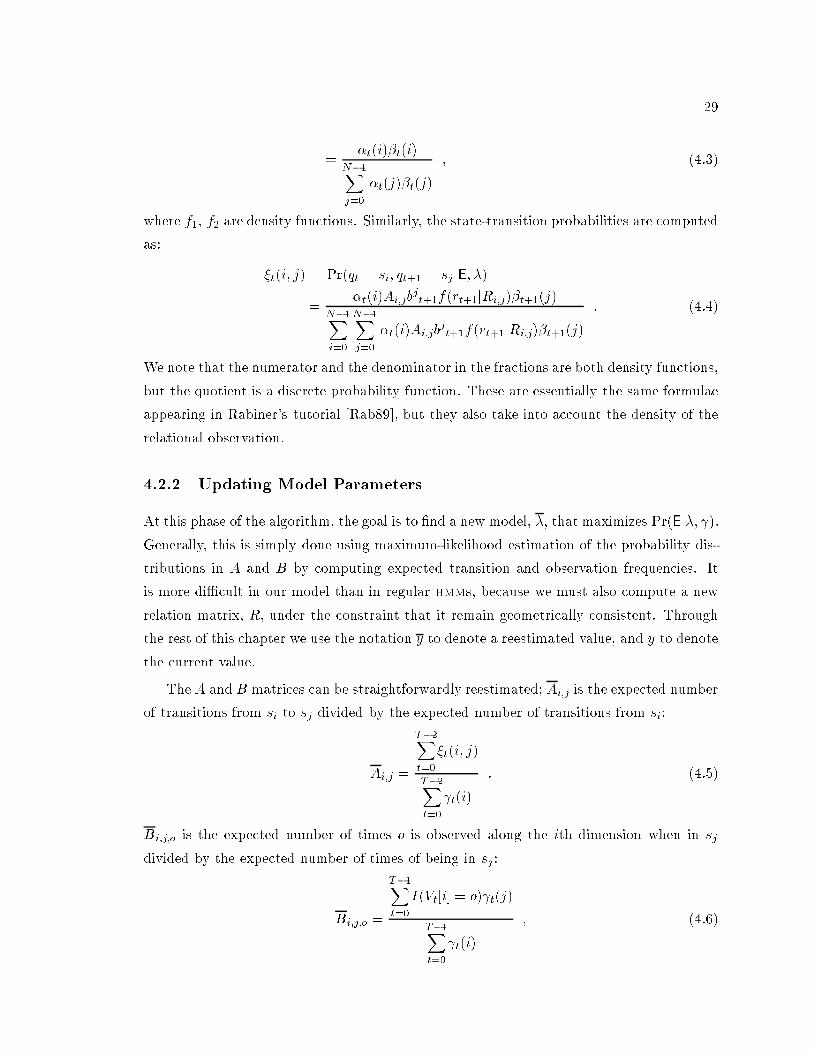
29= �t(i)�t(i)N�1Xj=0 �t(j)�t(j) ; (4.3)where f1; f2 are density fun tions. Similarly, the state-transition probabilities are omputedas: �t(i; j) = Pr(qt = si; qt+1 = sj jE; �)= �t(i)Ai;jbjt+1f(rt+1jRi;j)�t+1(j)N�1Xi=0 N�1Xj=0 �t(i)Ai;jbjt+1f(rt+1jRi;j)�t+1(j) : (4.4)We note that the numerator and the denominator in the fra tions are both density fun tions,but the quotient is a dis rete probability fun tion. These are essentially the same formulaeappearing in Rabiner's tutorial [Rab89℄, but they also take into a ount the density of therelational observation.4.2.2 Updating Model ParametersAt this phase of the algorithm, the goal is to �nd a new model, �, that maximizes Pr(Ej�; ).Generally, this is simply done using maximum-likelihood estimation of the probability dis-tributions in A and B by omputing expe ted transition and observation frequen ies. Itis more diÆ ult in our model than in regular hmms, be ause we must also ompute a newrelation matrix, R, under the onstraint that it remain geometri ally onsistent. Throughthe rest of this hapter we use the notation y to denote a reestimated value, and y to denotethe urrent value.The A and B matri es an be straightforwardly reestimated; Ai;j is the expe ted numberof transitions from si to sj divided by the expe ted number of transitions from si:Ai;j = T�2Xt=0 �t(i; j)T�2Xt=0 t(i) : (4.5)Bi;j;o is the expe ted number of times o is observed along the ith dimension when in sjdivided by the expe ted number of times of being in sj :Bi;j;o = T�1Xt=0I(Vt[i℄ = o) t(j)T�1Xt=0 t(i) ; (4.6)

30where I( ) is an indi ator fun tion with value 1 if is true and 0 otherwise.If we were not enfor ing geometri al onsisten y, the R matrix would be reestimated by:�mi;j def= �(Ri;j [m℄) = T�2Xt=0rt[m℄�t(i; j)T�2Xt=0 �t(i; j) (4.7)�mi;j def= �2(Ri;j [m℄) = T�2Xt=0 (rt[m℄� �mi;j)2�t(i; j)T�2Xt=0�t(i; j) ; (4.8)where m 2 fx; yg.However, the geometri al onstraints indu e interdependen ies among the optimal meanestimates as well as between optimal varian e estimates and mean estimates. Parameter es-timation under this form of onstraints is almost untreated in main-stream statisti s [Bar84℄and we found no previous existing solutions to the estimation problem we are fa ing. Asan illustration onsider the following onstrained estimation problem of 2 normal means.Example 4.1 Suppose we are given two sample sets of points P = fp1; p2; : : : ; png andQ = fq1; q2; : : : ; qkg. We are told that they were independently drawn from two distin tnormal distributions with means �P ; �Q and varian es �2P ; �2Q, respe tively. We are askedto �nd maximum likelihood estimates for the two distribution parameters. Moreover, we arealso told that the means of the two distributions are related, su h that �Q = ��P . Thissetting is shown in Figure 4.1.If not for the latter onstraint, the task is simple [DeG86℄, and we have:�P = Pni=1 pin ; �Q = Pkj=1 qjk ; �2P = Pni=1(pi � �x)2n ; �2Q = Pkj=1(qj � �y)2k : (4.9)However, the onstraint �P = ��Q for es us to �nd a single mean value � and set the otherone to its negated value, ��. Intuitively speaking, when hoosing su h a maximum likelihoodsingle mean, the sample that is more on entrated should have more e�e t and the samplethat varies more should be more \submissive". This way the overall sample deviation fromthe means would be minimized and the likelihood of the data maximized. Thus, there existsmutual dependen e between the estimation of the mean and the estimation of the varian e,as opposed to the estimation given in formulae 4.9, in whi h the optimal mean estimationdepends solely on the sampled values.

31-6 -4 -2 2 4 6

PQ

-8 -6 -4 -2 2 4 6 8

-7.5

-5

-2.5

2.5

5

7.5

P

QFigure 4.1: Examples of two sets of normally distributed points with onstrained means,in 1 and 2 dimensions.Sin e the samples are independently drawn, their joint likelihood fun tion is:f(P;Qj�P ; �Q; �2P ; �2Q) = nYi=1 e�(pi��P )22�2Pp2��P � kYj=1 e�(qj��Q)22�2Qp2��Q :The log of the joint likelihood fun tion under the onstraint �Q = ��P is therefore:nXi=1 �(pi � �P )22�2P � log(p2��P )!+ kXj=1 �(qj + �P )22�2Q � log(p2��Q)! : (4.10)By taking the derivatives of expression 4.10 with respe t to �P , �P and �Q and equatingthem to 0, while using the onstraint �Q = ��P , we obtain the following set of mutualequations for maximum likelihood estimators:�P = �2Q nXi=1pi � �2P kXj=1qjn�2Q + k�2P ; �Q = ��P ; �2P = nXi=1(pi � �P )2n ; �2Q = kXj=1(qj + �P )2k :By substituting the expressions for �P and �Q into the expression for �P , we obtain a ubi equation whi h is umbersome, hen e is not given here, but still solvable (in this simple ase). The solution provides a maximum likelihood estimate for the mean and varian eunder the above onstraint.In the ase where the two samples are assumed to have the same varian e, the varian efa tors in the expression for �P above an el out, and the estimate for �P is simply:�P = ��Q = nXi=1pi � kXj=1qjn + k ;

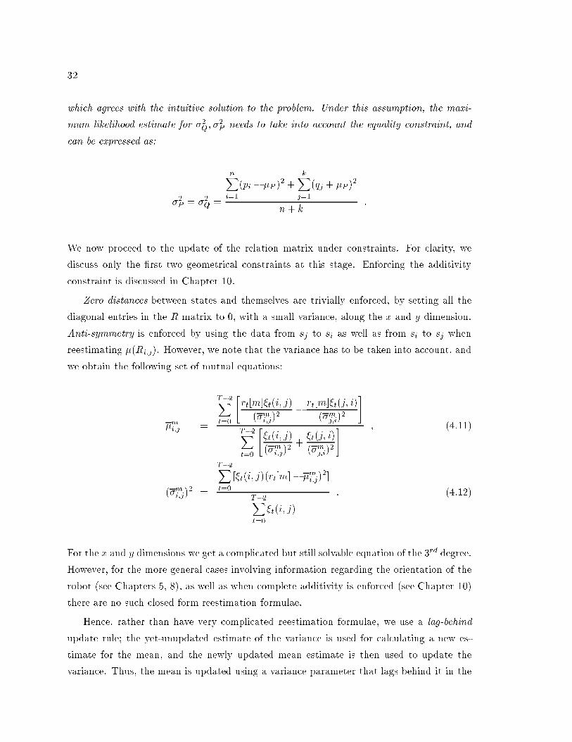
32whi h agrees with the intuitive solution to the problem. Under this assumption, the maxi-mum likelihood estimate for �2Q; �2P needs to take into a ount the equality onstraint, and an be expressed as: �2P = �2Q = nXi=1(pi � �P )2 + kXj=1(qj + �P )2n + k :We now pro eed to the update of the relation matrix under onstraints. For larity, wedis uss only the �rst two geometri al onstraints at this stage. Enfor ing the additivity onstraint is dis ussed in Chapter 10.Zero distan es between states and themselves are trivially enfor ed, by setting all thediagonal entries in the R matrix to 0, with a small varian e, along the x and y dimension.Anti-symmetry is enfor ed by using the data from sj to si as well as from si to sj whenreestimating �(Ri;j). However, we note that the varian e has to be taken into a ount, andwe obtain the following set of mutual equations:�mi;j = T�2Xt=0 "rt[m℄�t(i; j)(�mi;j)2 � rt[m℄�t(j; i)(�mj;i)2 #T�2Xt=0 "�t(i; j)(�mi;j)2 + �t(j; i)(�mj;i)2 # ; (4.11)(�mi;j)2 = T�2Xt=0 [�t(i; j)(rt[m℄� �mi;j)2℄T�2Xt=0�t(i; j) : (4.12)For the x and y dimensions we get a ompli ated but still solvable equation of the 3rd degree.However, for the more general ases involving information regarding the orientation of therobot (see Chapters 5, 8), as well as when omplete additivity is enfor ed (see Chapter 10)there are no su h losed form reestimation formulae.Hen e, rather than have very ompli ated reestimation formulae, we use a lag-behindupdate rule; the yet-unupdated estimate of the varian e is used for al ulating a new es-timate for the mean, and the newly updated mean estimate is then used to update thevarian e. Thus, the mean is updated using a varian e parameter that lags behind it in the

33update pro ess, and the reestimation formula 4.11 needs to use �mi;j rather than �mi;j :�mi;j = T�2Xt=0 "rt[m℄�t(i; j)(�mi;j)2 � rt[m℄�t(j; i)(�mj;i)2 #T�2Xt=0 "�t(i; j)(�mi;j)2 + �t(j; i)(�mj;i)2 # : (4.13)A possible alternative to our lag-behind approa h is to update the mean as though theassumption �j;i = �i;j indeed holds. Under this assumption, the varian e terms in equa-tion 4.11 an el out, and the mean update is independent of the varian e on e again. Thenthe varian es are updated as stated in equation 4.12, without assuming any onstraints overthem. This approa h was taken in earlier stages of this work [SK97b, SK98℄. We experimen-tally studied various update poli ies for learning onstrained Gaussian parameters1. Theexperimental results under the restri ted experimental settings suggest that the lag-behindstrategy is superior to the others and very lose to the a tual maximum likelihood estima-tion method. Moreover, a similar approa h was taken by other resear hers when using emin highly non-linear optimization problem, termed one step late update [MK97℄. It turnsout, as we also show in Se tion 4.3.3, that this update approa h falls under the generalizedem family of algorithms, whi h have similar properties to the em algorithms.The omplexity of the above algorithm per iteration is still O(TN2), like the standardBaum-Wel h method. Note that the onstants are signi� ant here, sin e the al ulation offormulae 4.1 and 4.2 requires the evaluation of exponential terms, whi h is a time onsumingoperation. This ost an be signi� antly redu ed through the use of lookup-tables, althoughthis is not urrently implemented in our ode.4.2.3 Stopping CriterionAs stated in the beginning of this se tion, and proved in Se tion 4.3, our algorithm is anem algorithm and as su h it is guaranteed to onverge to a lo al maximum of the likelihoodfun tion. Moreover, a lo al maximum is rea hed if and only if the model parameters haverea hed a �xed point and are no longer hanged by the reestimation pro edure.To pra ti ally determine that the algorithm has indeed onverged, we an ompare thevalue of the likelihood fun tion between onse utive iterations. When the hange in the1I am grateful to Luis Ortiz for lending his ode and expertise, as well as for ondu ting these experimentswith me.

34likelihood value is less than a predetermined small �, we an assume that onvergen e hasbeen rea hed, and stop the algorithm.Alternatively, we an ompare the amount of hange in the model parameters themselvesbetween iterations, and when the hange in ea h parameter is less than a predetermined �,de ide that a �xed point has been rea hed, whi h implies the onvergen e of the algorithm.Note that the odometri data and the odometri relation matrix are used as an aid to-wards obtaining the transition and observation matri es, and therefore, a stopping riterionneed only take into onsideration the transition and observation matri es or the likelihoodof the observation data, rather than the relation matrix or the likelihood of the odometri data.The latter of the two stopping riteria an be viewed as more onservative. The reason isthat the likelihood fun tion expression involves a produ t of the model's parameters [Rab89℄.Sin e these parameters are all probabilities (as we are only taking into a ount the transitionand observation distribution matri es), they are all numbers between 0 and 1. Therefore,when the hange in ea h of them is less than �, the hange in the likelihood value is typi allymu h smaller.In our implementation of the algorithm, we use this se ond riterion, and determinethat the algorithm has onverged when the hange in ea h of the entries of the transitionmatrix, A, and the observation matrix, B, from one iteration to the next does not ex eed aprede�ned �. (We set � = 0:001 in our implementation). By omparing only the hange inthe transition and observation matri es, we also enable a fair omparison of the number ofiterations required for onvergen e with and without the use of odometri information, asdes ribed in Chapters 7 and 9 of this work.4.2.4 Extending the Algorithm for Learning POMDPsTo extend the algorithm given above to learn a omplete pomdp, ea h item in the experien esequen e E ontains, in addition to the observation and the odometri relation, the a tionthat aused the transition asso iated with the odometri relation.For ea h a tion there is a separate pair of matri es A and B. Hen e, the forward-ba kward pro edure as des ribed in Se tion 4.2.1, and in parti ular Equations 4.1 and 4.2,must take into a ount at ea h time t the transition probabilities Aij and the observationprobabilities bj that are asso iated with the spe i� a tion taken at time t. Furthermore,the update pro edure for the A and B matri es, (formulae 4.5 and 4.6), for a parti ular

35a tion a, only takes into a ount the estimated state transitions and observations that area result of a in the data sequen e. The update of the relation matrix R does not need totake any a tion information into a ount sin e R is a single ommon matrix for the wholemodel.The time omplexity of learning a pomdp ompared with that of learning an hmm isnot signi� antly di�erent sin e the forward-ba kward pro edure des ribed in Se tion 4.2.1,whi h is the most omputationally-intensive part of the algorithm, does not require anyadditional omputational steps. The only di�eren e in this pro edure is the one mentionedabove. Only the �nal update of the A and B matri es, needs to be performed separately forea h a tion, but this stage is not a omputational bottlene k. Therefore, the overall timerequirements remain almost un hanged, under the assumption that the number of possiblea tions is typi ally mu h smaller than the number of states in the model. A fa tor that islikely to make learning a pomdp more time onsuming, and needs to be taken into a ount,is the larger number of model parameters introdu ed due to the multiple a tions. In order tofa ilitate the learning of useful models, longer data sequen es, and therefore proportionallymore omputation time, may be required.4.3 Corre tness Proof of the Reestimation FormulaeFor the kind of iterative reestimation algorithms that we use, proving the orre tness of thereestimation formulae means proving that through repeated reestimation, the likelihooddoes not de rease, and that the algorithm onverges to a �xed-point model �, whi h isa lo al maximum of the likelihood fun tion P (Ej�), where E is the observed experien esequen e. We formalize this in the following theorem:Theorem 4.1 Let �0 be the urrent model, E be the experien e sequen e, and � be thereestimated model a ording to the reestimation formulae 4.5, 4.6, and either 4.7 and 4.8,or 4.13 and 4.12. Then Pr(Ej�0) � Pr(Ej�), and �0 = � if and only if �0 is a lo al maximumof Pr(Ej�) as a fun tion of �.Proof: There are several proof te hniques for the orre tness of the reestimation for-mulae for the standard Baum-Wel h algorithm (under various kinds of observation matrixB) [BPS+70, DLR77, LRS83, Jua85, JLS86℄. Our proof uses the same approa h as thelatter two. It is straightforward to show that maximization of the likelihood fun tion withrespe t to ea h of the parameters separately is equivalent to its maximization with respe t

36the omplete model. Hen e, we break up the proof, and prove that ea h of the reestimationformulae indeed improves the likelihood fun tion with respe t to the asso iated reestimatedparameter. Sin e the likelihood fun tion with respe t to the A and B matri es is a dis reteprobability distribution, it is bounded from above, and the onvergen e of the pro ess isguaranteed. For the relation matrix reestimation pro edure, onvergen e is also guaran-teed through a more ompli ated ondition given by Wu [Wu83℄, and whi h holds for theexponential family of distributions [MK97℄. Hen e onvergen e is guaranteed.4.3.1 Transitions and ObservationsTo prove the orre tness of formulae (4.5) and (4.6), we use the entral theorem of Baumand Sell [BS68℄, whi h states2 that for x = fxijg s.t. xij > 0; 0 � j � N � 1, andPN�1j=0 xij = 1, given a homogeneous polynomial P in the variable xij, with nonnegative oeÆ ients, the transformation xij = xij �P�xijN�1Xk=0xik �P�xik (4.14)satis�es P (x) � P (x), and x = x if and only if x is a lo al maximum of P .The density expression Pr(Ej�) = PN�1i=0 �T�1(i) = PN�1i=0 �T�1(i)�T�1(i) , whi h wewant to maximize, is indeed a homogeneous polynomial in Aij and in Bijo. Both Aij andBijo are dis rete probability distributions, therefore are positive and satisfy PN�1j=0 Aij = 1and Po2Oi Bijo = 1 . Hen e, a ording to the above theorem the reestimation formula forAij , that leads to a lo al maximization of P (EjAij) is:Aij = Aij �P (Ej�)�AijN�1Xk=0Aik �P (Ej�)�Aik : (4.15)We now need to show that the right-hand side of formula (4.15) is equal to that of (4.5).To do this we need to show that:�P (Ej�)�Aij = T�2Xt=0�t(i)bjt+1f(rt+1jRi;j)�t+1(j) : (4.16)By substituting the right hand side expression into (4.15), and using equations (4.3,4.4) weget the desired equality.2Baum and Sell's theorems are a tually somewhat stronger and the statement given here is just one onsequen e.

37By indu tion on k; 0 � k � T � 1, it is easy to show that:N�1Xi=0 ��k(i)�Aij �k(i) = k�1Xt=0�t(i)bjt+1f(rt+1jRi;j)�t+1(j) :For k = T � 1 we get (4.16), whi h on ludes the proof of formula (4.5). The proof for Bijo(formula (4.6)) is almost identi al.4.3.2 Odometri RelationsWe note that the density expression, Pr(Ej�), is not a polynomial in �(Ri;j [m℄) and�2(Ri;j [m℄). Hen e the theorem by Baum and Sell an not be applied here. Still, sin e weassume that the odometri relations along the x and y dimensions are normally distributed,in the un onstrained ase, their reestimation pro edure is an instan e of the exponentialfamily reestimation, dis ussed by Dempster et al [DLR77℄. However, for the sake of om-pleteness and for an easier dis ussion of the onstrained ase, we provide a omplete proof,using the te hnique of maximizing Baum's auxiliary fun tion, following Se tion 4 of thepaper by Baum et al. [BPS+70℄. We denote by ��, where � is some relation matrix , themodel whose A and B matri es are the same as those of �, but whose relation matrix R isrepla ed by the matrix �.We start by making the observation that if S is the set of all state sequen es of length T ,i.e. S = fsg where s = s0; : : : ; sT�1 is a sequen e of states of length T , the density P (Ej�) an be expressed as P (Ej�) =Xs2S P (E; s j�) =X

s2S P (Ejs ; �)P (s j�) :We an rewrite P (Ejs ; �) and P (s j�) asP (Ejs ; �) = T�1Yt=0 bstt T�1Yt=1 f(rtjRst�1;st) and P (s j�) = �s0 T�1Yt=1 Ast�1;st :Thus, P (Ej�) an be expressed asXs2S �(s ) T�1Yt=1 f(rtjRst�1;st) ;where �(s ) is a produ t of initial, transition and observation probabilities. Re alling thatf(rtjRi;j) denotes the density of rt a ording to the D-variate independent normal distri-bution with the parameters stored in Ri;j, we rewrite it asf(rtjRi;j) = DYm=1 fmij (rmt )p2��mij ; (4.17)

38where rmt def= rt[m℄ and fmij (rmt ) def= e�(rmt ��mij )2=2(�mij )2 . We also use the notation:fmij (rmt ) def= e�(rmt ��mij )2=2(�mij )2 and fij(rt) def= QDm=1 fmij (rmt ).Baum et al. [BPS+70℄ introdu e an auxiliary fun tion, Q, and prove that maximizing itis the same as in reasing the likelihood. More formally, the R that maximizes the auxiliaryfun tion Q(R;R) def= Xs2S P (E; s j�) log(T�1Yt=1 f(rtjRst�1;st))= Xs2S P (E; s j�) T�1Xt=1 log(f(rtjRst�1;st))also satis�es P (Ej�R) � P (Ej�R).Sin e the R that maximizes Q(R;R) also maximizes the same expression in whi hp2�fmij (rmt ) is substituted for fmij (rmt ), we an ignore the p2� fa tor in (4.17) and rewriteQ as Q(R;R) =X

s2S P (E; s j�) T�1Xt=1 DXm=1[log(fmst�1;st(rmt ))� log(�mst�1;st)℄ : (4.18)Sin e the normal distribution is stri tly log- on ave, a slight adaptation to the proof of The-orem 4:1 in [BPS+70℄ is suÆ ient for showing that Q above has a unique global maximumas a fun tion of �mij and �mij , whi h is the unique point in whi h the partial derivatives of Qa ording to �mij and �mij are 0. We now show that the reestimation formulae (4.7) and (4.8)indeed �nd the maximizing �mij and �mij .For a pair of states i; j and an odometry omponent m 2 fx; yg we an express the re-stri tion of the auxiliary fun tion Q to transitions from i to j and to the mth odometri omponent, m, asQmij (R;R) =Xs2S P (E; s j�) Xt s.t.st�1=ist=j (log(fmst�1;st(rmt ))� log(�mst�1;st)) :Observing that �t�1(i; j) = X

s2S s.t.st�1=ist=j P (E; s j�) allows us to rewrite Qmij (R;R) asQmij (R;R) = T�2Xt=0 �t(i; j)(log(fmi;j(rmt+1))� log(�mij )) : (4.19)Sin e �Q��mij = �Qmij��mij and �Q��mij = �Qmij��mij , showing that the partial derivatives of Qmij with respe tto �mij and �mij are 0 whenever equations (4.7) and (4.8) are satis�ed, on ludes our proof.The di�erentiation is straightforward and is provided in Appendix B.1 .

394.3.3 Constrained Odometri RelationsThe orre tness of formulae 4.13 and 4.12, under our lag-behind update poli y, is proved byshowing that these update rules are instan es of generalized em. Dempster et al. [DLR77℄introdu ed this notion, and it is explained in detail by M La hlan and Krishnan [MK97℄.The idea is that by merely improving the auxiliary fun tion Q, rather than maximizing it,at ea h iteration, we are still guaranteed to improve the likelihood fun tion. Therefore, itis not ne essary to �nd an update rule that maximizes Q but simply one that improves it.The proof te hnique presented here uses dire t enfor ement of the anti-symmetry onstraintin the expression for Q. This is in ontrast to the use of Lagrange multipliers in earlierwork [SK97a℄.From equations (4.18) and (4.19) we have:Q(R;R) = N�1Xi=0 N�1Xj=0 DXm=1Qmij (R;R) : (4.20)By isolating all terms in whi h i = j we an rewrite this expression as:Q(R;R) = N�1Xi=0 DXm=1Qmii (R;R) + N�1Xi=0 N�1Xj=(i+1) DXm=1[Qmij (R;R) + Qmji(R;R)℄ : (4.21)In order to in rease the sum in (4.21), under the onstraint �mij = ��mji , with respe t tothe parameters �mij and �mij , it is suÆ ient to in rease the sum of ea h pair (Qmij (R;R) +Qmji(R;R)) with respe t to these parameters, sin e all other pairs do not ontain them.Thus, we are left with the following expression:Lmij (�mij ; �mji ; �mij ; �mji )= T�2Xt=0 264�t(i; j)0B�log(e� (rmt ��mij )22(�mij )2 )� log(�mij )1CA + �t(j; i)0B�log(e� (rmt ��mji )22(�mji )2 )� log(�mji)1CA375 :We enfor e the anti-symmetry onstraint by substituting �mji by ��mij in the above expres-sion, and obtain the following expression whi h we need to in rease with respe t to �mij , �mijand �mji :

40Lmij (�mij ; �mij ; �mji)= T�2Xt=0 264�t(i; j)0B�log(e� (rmt ��mij )22(�mij )2 )� log(�mij )1CA+ �t(j; i)0B�log(e� (rmt +�mij )22(�mji )2 )� log(�mji)1CA375= T�2Xt=0 "�t(i; j) �(rmt � �mij )22(�mij )2 � log(�mij )!+ �t(j; i) �(rmt + �mij )22(�mji)2 � log(�mji)!# :Let �mij ; �mij and �mji be the urrent values of the parameters. To in rease Lmij we do thefollowing:1. Temporarily �x �mij ; �mji to be the urrent �mij ; �mji . Denote by bLmij (�mij ) the fun tionobtained from Lmij through this instantiation of the � parameters. Formally stated:bLmij (�mij ) def= Lmij (�mij ; �mij ; �mji ) :2. Find the value b�mij that maximizes bLmij (�mij ).3. Set �mij in Lmij to the value b�mij found in step 2. Denote by bbLmij (�mij ; �mji) the fun tionobtained from Lmij through this instantiation of �mij . Formally stated:bbLmij (�mij ; �mji) def= Lmij (b�mij ; �mij ; �mji) :4. Find values b�mij ; b�mji that maximize bbLmij .5. Set �mij ; �mji to be b�mij ; b�mji .Sin e b�mij maximizes bLmij (�mij ) we have:Lmij (b�mij ; �mij ; �mji ) � Lmij (�mij ; �mij ; �mji ) :Sin e b�mij ; b�mji maximize bbLmij (�mij ; �mji) we have:Lmij (b�mij ; b�mij ; b�mji ) � Lmij (b�mij ; �mij ; �mji ) :By transitivity: Lmij (b�mij ; b�mij ; b�mji ) � Lmij (�mij ; �mij ; �mji ) :Hen e, setting �mij ; �mij ; �mji a ording to the above pro edure does not de rease Lmij . If itdoes not stri tly in rease Lmij , then a ording to the generalized em algorithm a maximumof the likelihood fun tion is rea hed.It is now left to obtain expressions for b�mij ; b�mij , and b�mji .

41To �nd b�mij , we take the derivative of bLmij (�mij ) with respe t to �mij and equate it to 0.� bLmij��mij = T�2Xt=0 [�t(i; j)(rmt � �mij )(�mij )2 � �t(j; i)(rmt + �mij )(�mji )2 ℄ :By equating to 0 we get: �mi;j = T�2Xt=0 [rmt �t(i; j)(�mi;j)2 � rmt �t(j; i)(�mj;i)2 ℄T�2Xt=0 [�t(i; j)(�mi;j)2 + �t(j; i)(�mj;i)2 ℄ ;whi h is identi al the reestimation expression for �mi;j given in 4.13. It is easy to he k thatthe se ond derivative of bLmij (�mij ) with respe t to �mij is negative, and therefore this is indeeda maximum rather than a minimum.Similarly, to obtain b�mij , we take the derivative of bbLmij (�mij ; �mji) with respe t to �mij , andequate it to 0, and a similar pro ess is done for �nding b�mji . The obtained expressions are:(�mi;j)2 = T�2Xt=0 [�t(i; j)(rt[m℄� �mi;j)2℄T�2Xt=0 �t(i; j) (�mj;i)2 = T�2Xt=0 [�t(j; i)(rt[m℄ + �mi;j)2℄T�2Xt=0 �t(j; i) :whi h agree with the update formulae 4.12. Again, the se ond derivative is negative, whi hensures that this is indeed a maximum point. This on ludes our proof. 2For the spe ial ase where i = j , the value �mij is 0, whi h shows that the update formulaindeed satis�es the �rst two of the three geometri al onsisten y onstraints.

42

Chapter 5Dire tional Data and Distributions5.1 MotivationThroughout our dis ussion so far, we have onsidered only two omponents of the odometri information gathered by the robot, namely, the x and y oordinates. However, an additionalmeasure that is usually re orded is the hange of the robot's heading, �, as it moves fromone state to the next. If a robot is standing in one position and takes the a tion of turningleft or right, a respe tive hange of heading of approximately �90Æ is re orded between thestate prior to the turn and the state following the turn. Obviously, there is noise around thismeasure, as is the ase for the x and y measures. In previous work [SK97b, SK97a℄, we didtreat the hange in heading as though it were simply normally distributed. However, the hange in heading is di�erent from that in x and y, in the sense that angular measurementsare y li . That is, a hange in heading of 90Æ is the same as a hange of 450Æ or of �270Æ.If we knew in advan e, for every two states, the approximate hange in heading (��)that the robot goes through when moving from one of them to the other, we ould stillhave modeled it as though it were approximately normal with a mean ��, and some smallvarian e �2 [AC82℄. We ould adopt a onvention of having all angles normalized to bewithin a y li range, e.g. [�180Æ; 180Æ℄, (similarly we may use radians or other units),and always hoose to take as the angular hange between two points min(j�j; 360Æ � j�j),and assign it the orre t sign. However, we do not know in advan e the angular hangebetween every two states. We have a sequen e of angular measurements and we estimatethe probabilities of the states in whi h they were re orded, and take a weighted mean of themeasurements in order to estimate the angular hange between every two states. Thus, weare fa ing the following problem: What is the interpretation of a \mean angle"?43

44baFigure 5.1: Robot hanges heading from state a to state b.As an example, onsider the transition from state a to state b, as depi ted in Figure 5.1.Suppose that we adopt the onvention that angles are expressed as numbers between �180Æand 180Æ. Also, suppose we have two (noisy) measurements of the angular distan e fromstate a to state b: �169Æ and 185Æ. The simple average between these two measurementsgives us an estimate of the mean heading hange of 8Æ. Obviously this is not the value thatre e ts even remotely the hange of heading between the two states. A similar problemarises if we use a onvention for expressing angles between 0Æ and 360Æ. The problem lies inthe fa t that angles that are about 180Æ away from the mean angle greatly deviate from thismean, while angles that are about 360Æ away from the mean are a tually very lose to it.To apture this idea, the on ept of ir ular distribution is required. Angular data plays asigni� ant role in various aspe ts of both theory and me hani s of roboti s, as well as otherareas of omputer s ien e (e.g omputer graphi s). Sin e distributions over su h data arenot widely known to resear hers in this area, (although the problemati aspe t of su h datahas long been realized by statisti ians), we provide here a brief introdu tion to the basi on epts and te hniques used for handling ir ular data. In parti ular we on entrate onthe von Mises distribution, whi h is a ir ular version of the normal distribution. Furtherdis ussion an be found in several statisti al publi ations [GGD53, Mar72, KJ82a, KJ82b℄.Se tion 5.4 returns to show how the theory is applied in our model and learning algorithm.5.2 Statisti s of Dire tional DataDire tional data in the 2-dimensional spa e an be represented as a olle tion of 2-dimensionalve tors, fhx1; y1i; : : :hxn; ynig, on the unit ir le, as shown in Figure 5.2. The 2-dimensionalpoints an also be represented as the orresponding angles between the radii from the enterof the unit ir le and the x axis, (�1; : : : ; �n), respe tively. The relationship between thetwo representations is:xi = os(�i); yi = sin(�i); (1 � i � n) :The ve tor mean of the n points, hx; yi, is al ulated as:

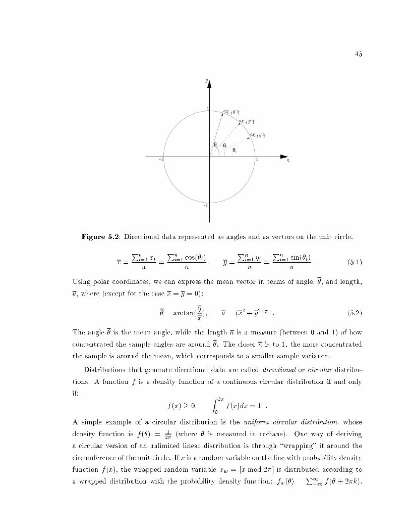
4511

<x , y >

33<x , y >

22<x , y >

θ2θ3

θ1

x

y

1

-1

-1 1Figure 5.2: Dire tional data represented as angles and as ve tors on the unit ir le.x = Pni=1 xin = Pni=1 os(�i)n ; y = Pni=1 yin = Pni=1 sin(�i)n : (5.1)Using polar oordinates, we an express the mean ve tor in terms of angle, �, and length,a, where (ex ept for the ase x = y = 0):� = ar tan(yx); a = (x2 + y2) 12 : (5.2)The angle � is the mean angle, while the length a is a measure (between 0 and 1) of how on entrated the sample angles are around �. The loser a is to 1, the more on entratedthe sample is around the mean, whi h orresponds to a smaller sample varian e.Distributions that generate dire tional data are alled dire tional or ir ular distribu-tions. A fun tion f is a density fun tion of a ontinuous ir ular distribution if and onlyif: f(x) � 0; Z 2�0 f(x)dx = 1 :A simple example of a ir ular distribution is the uniform ir ular distribution, whosedensity fun tion is f(�) = 12� (where � is measured in radians). One way of derivinga ir ular version of an unlimited linear distribution is through \wrapping" it around the ir umferen e of the unit ir le. If x is a random variable on the line with probability densityfun tion f(x), the wrapped random variable xw = [x mod 2�℄ is distributed a ording toa wrapped distribution with the probability density fun tion: fw(�) = P1�1 f(� + 2�k).

46Applying this derivation to the normal distribution results in a ir ular version of the normaldistribution, but estimating its parameters from sample data an be problemati [GGD53,Mar72℄.An easier-to-estimate ir ular version of the normal distribution was derived by vonMises [GGD53, Mar72℄, in a way analogous to the way Gauss derived the linear normaldistribution | whose maximum-likelihood parameter estimates are the sample mean andvarian e. This ir ular distribution is the one we are using to model the robot heading inthis work, and is des ribed below.5.3 The von Mises DistributionA ir ular random variable, �, 0 � � � 2�, is said to have the von Mises distribution withparameters � and �, where 0 � � � 2� and � > 0, if its probability density fun tion is:f�;�(�) = 12�I0(�)e� os(���) ;where I0(�) is the modi�ed Bessel fun tion of the �rst kind and order 0:I0(�) = 1Xr=0 1r!2 (12�)2r :Similar to the linear normal distribution, this is a unimodal distribution, symmetri alaround �. The mode is at � = � while the antimode is at � = � + �. We observe that theratio of the density at the mode to the density at the antimode is e2�, whi h indi ates thatthe larger � is, the more on entrated the density is about the mode. Figure 5.3 shows an\unwrapped" plot of the von Mises distribution for various values of � where � = 0.We now des ribe how to estimate the parameters � and � given a set of heading samples,angles �1; : : :�n, from a von Mises distribution. We are looking for maximum likelihoodestimates for � and �. The likelihood fun tion for the data generated by a von Misesdistribution with parameters � and � an be expressed as:L�;� = nYi=1 f�;�(�i) = e(�Pni=1 os(���i))(2�)nI0(�)n :Hen e the log likelihood islog(L�;�) = � nXi=1 os(�� �i)� log((2�)nI0(�)n) :

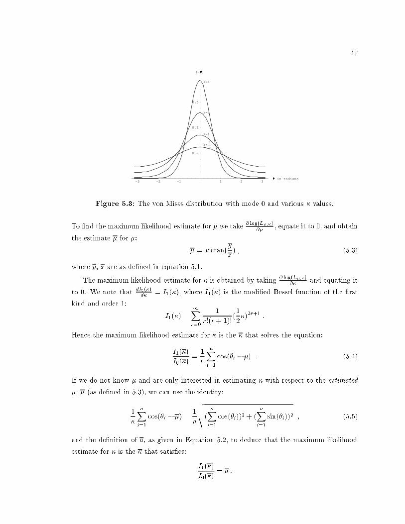
47-3 -2 -1 1 2 3

in radians

0.2

0.4

0.6

f( )

k=1

2

k=1

k=2

k=4

PSfrag repla ements�

�Figure 5.3: The von Mises distribution with mode 0 and various � values.To �nd the maximum likelihood estimate for � we take � log(L�;�)�� , equate it to 0, and obtainthe estimate � for �: � = ar tan(yx) ; (5.3)where y, x are as de�ned in equation 5.1.The maximum likelihood estimate for � is obtained by taking � log(L�;�)�� and equating itto 0. We note that dI0(�)d� = I1(�), where I1(�) is the modi�ed Bessel fun tion of the �rstkind and order 1: I1(�) = 1Xr=0 1r!(r+ 1)!(12�)2r+1 :Hen e the maximum likelihood estimate for � is the � that solves the equation:I1(�)I0(�) = 1n nXi=1 os(�i � �) : (5.4)If we do not know � and are only interested in estimating � with respe t to the estimated�, � (as de�ned in 5.3), we an use the identity:1n nXi=1 os(�i � �) = 1nvuut( nXi=1 os(�i))2 + ( nXi=1 sin(�i))2 ; (5.5)and the de�nition of a, as given in Equation 5.2, to dedu e that the maximum likelihoodestimate for � is the � that satis�es: I1(�)I0(�) = a :

48However, if we do have a given � and we want to �nd a maximum likelihood estimate forthe on entration � of the sample data around that spe i�ed �, the identity 5.5 annot beused (see also Upton [Upt73℄). We need to use as a maximum likelihood estimate for �, the� that satis�es:I1(�)I0(�) = max[ 1n nXi=1 os(�i��); 0℄ = max24 1nvuut( nXi=1 os(�i))2 + ( nXi=1 sin(�i))2 � ( nXi=1 sin(� � �i)); 035 :The above estimation formulae agree with the intuition that the sample is more on entrated(� is larger) about the sample mean, �, than about the true distribution mean, �.5.4 Handling Angular Odometri ReadingsIt is now left to explain how we use the von Mises distribution to model the heading readingsobtained by the robot as part of its odometri information. Through the rest of this se tionwe explain how the parameters of the von Mises distribution are in orporated into thehidden Markov model and how the learning algorithm des ribed in Chapter 4 is adapted tolearn these parameters.To model the heading di�eren e between ea h pair of states, the relation matrix R,des ribed in Se tion 3.2, be omes 3-dimensional rather than 2-dimensional, onsisting of the omponents hx; y; �i rather than just hx; yi. The omponent Ri;j[�℄ represents the heading hange when moving from state si to sj , and is assumed to onsist of the two parameters ofthe von Mises distribution governing this hange. The notation ��i;j def= �(Ri;j [�℄) representsthe mean of the distribution for this heading hange, while ��i;j def= �(Ri;j[�℄) represents the on entration parameter around the mean. The three onstraints stated in Se tion 3.2 forthe omponents of R, hold for the � omponent as well.Similarly, every observed relation item, rt, in the experien e sequen e E, has a heading- hange omponent, �, whi h re ords the hange in heading of the robot between the stateat time t, qt, and the state qt+1.The reestimation formula for the von Mises mean and on entration parameters of theheading hange between states si and sj is the solution to the equations:��i;j = ar tan0BBBBB� T�2Xt=0 [sin(rt[�℄)(�t(i; j)�i;j � �t(j; i)�j;i)℄T�2Xt=0 [ os(rt[�℄)(�t(i; j)�i;j + �t(j; i)�j;i)℄1CCCCCA

49I1[��i;j ℄I0[��i;j ℄ = max"PT�2t=0 [�t(i; j) os(rt[�℄� ��i;j)℄PT�2t=0 �t(i; j) ; 0# : (5.6)Note here that the larger �ij is, the more on entrated the sample is around the mean, andthe more weight we give to the estimated ounts �t(i; j) of observing this mean. Also notethat the denominator ontains a sum rather than a di�eren e, sin e os is an even fun tionand os(�rt[�℄) = os(rt[�℄).Rather than try to solve these hard mutual equations, we take advantage of generalizedem as we did in Se tion 4.3.2, and use the \lag-behind" update. We update the mean usingthe urrent estimates of the on entration parameters, �i;j ; �j;i, as follows:��i;j = ar tan0BBBBB� T�2Xt=0 [sin(rt[�℄)(�t(i; j)�i;j � �t(j; i)�j;i)℄T�2Xt=0 [ os(rt[�℄)(�t(i; j)�i;j + �t(j; i)�j;i)℄1CCCCCA ;and then al ulate the new on entration parameters based on the newly updated mean,as the solution to equation 5.6. Finding ��i;j that satis�es this equation is done through theuse of a lookup table, listing values of the quotient I1[x℄I0[x℄ .The above reestimation formulae agree with the maximum likelihood estimator formulaegiven in equations (5.3, 5.4). The onvergen e of the estimation pro ess is guaranteed dueto the von Mises being a member of the exponential family [Mar72℄, and the monotoneimprovement of the likelihood through their use an be proved along the lines of the proofprovided in Se tion 4.3.3.

50

Chapter 6Choosing an Initial ModelIt is typi al in instan es of the Baum-Wel h algorithm to simply initialize the model atrandom, perhaps trying multiple initial models to �nd di�erent lo al likelihood maxima.Con retely, to hoose an N -state model uniformly at random, we �rst hoose N dis reteprobability distributions over N events, from the set of all possible N -dimensional proba-bility distributions, uniformly at random1, in order to onstru t the transition-distributionmatrix A; similarly, we hoose N distributions over observations for the observation matrixB; �nally we populate the relation matrix with random means, while enfor ing onsisten y onstraints.It is important to note that when ontinuous distributions are estimated, arbitrary ini-tialization of means and varian es an ause numeri al instability throughout the algorithm.For instan e, if an odometri relation between state i and state j is initially assigned a dis-tribution with an arbitrary mean that is far from any of the a tual odometri readings, withonly a small varian e around it, the density mass assigned to any odometri data a ord-ing to this distribution is very small, and an ex eed the ma hine's pre ision, ausing anunder ow to o ur. It is espe ially severe in a multi-dimensional odometri readings set-ting, like the one we are dealing with, sin e when numbers are multiplied by one another,even plausible density values rapidly de rease. Moreover, very small probability values ex- lude plausible state transitions between states i and j from being onsidered sin e theyare assigned a density mass whi h is arbitrarily lose to 0.We may try to hoose an initial large varian e for the odometri distribution, thus1See Cassandra's Ph.D. thesis [Cas98℄ for details on hoosing distributions at random.51

52avoiding the under ow problem. Su h an approa h results in highly ina urate mean rees-timation; if the odometry from state i to state j is initially estimated at a value with highvarian e, many transitions that do not go from i to j still get a reasonably high densityunder the distribution from i to j. When the mean is reestimated, all these transitionswould parti ipate in the al ulation. Thus the model redu es to having arbitrary meansthat roughly a ommodate all the data points due to the large varian e around them.This problem has long been realized by Rabiner et al. [RJL+85℄, and they make twosuggestions for a solution:� When events have very low density mass, add some small onstant to it.� Start from a good initial model.The �rst suggestion is lose in pra ti e to the Bayesian approa h, with a uniform prior overall events. This approa h is adopted in our implementation, as we add a small onstantto the estimated transition and o upation probabilities � and , to avoid 0 probabilities.However, as Rabiner et al. point out, it is not suÆ ient, sin e without good estimates formost of the parameters, all the data has low probability whi h is ompensated for by theadded onstants, resulting in a very at model. The overall e�e t is similar to that of havinga large varian e around arbitrary means.The se ond suggestion is not easily met, sin e we rarely have enough prior knowledgeto provide a good initial model, and as stated earlier, our goal is to automate as mu h aspossible the learning pro ess, avoiding the hard work of manually obtaining a good initialmodel.We have ome up with three initialization strategies. One is to use random initial distri-butions for the transition and observation matrix, and random relation means from withinthe range of odometri readings, assigning large initial varian e. All three geometri al on-straints are enfor ed on the relation means through dependen y propagation. For instan e,on e we pi k the mean �xij at random, the mean �xji is set to ��xij rather than hosenat random itself. This method still often leads to numeri al instability of the algorithm,and results in very at models, both in the sense of being lose to uniform transition andobservation distributions and in terms of ina urate odometri mean estimates with highvarian e around them.The two other initialization strategies are biased by the odometri data. One of themwas brie y des ribed in earlier publi ations [SK97b, SK97a℄, and is based on lustering

53states a ording to their odometri lo ations in a global oordinate system. This methodis not robust in the fa e of umulative rotational errors, whi h are dis ussed in Chapter 8.We also developed another initialization algorithm, based on lustering odometri rela-tions rather than positions, and on tagging ea h odometri relation by its estimated originand destination states. The algorithm is only on erned with odometri relations betweenstates, and therefore is not sensitive to umulative rotational errors. It also has the poten-tial advantage that it may assist in determining the number of states in the model when allwe have is a rough overestimate for this number.In the following we present both algorithms. They both take as input the sequen es Eof observations re orded at states and odometri relations re orded between states, as wellas the number of states N .6.1 K-Means-Based InitializationGiven a sequen e of observations and odometri readings E, we begin by assigning globalmetri oordinates to ea h element in the sequen e. This is done by a umulating theobserved odometri relations between onse utive pairs of odometri readings, as demon-strated in the following example.Example 6.1 Suppose we have the following 8 onse utive odometri readings:h2 94 92i; h1994 0 88i; h3 �93 86i; h�1999 �1 94i; h�4 102 91i;h1998 �5 90i; h�2 �106 91i; h�2003 7 87i :These an be viewed as the hange in heading from one state to the next measured within aglobal oordinate system.By a umulating these measures, assuming that the initial position is h0 0 0i we get thefollowing sequen e of global position assignments:h0 0 0i; h2 94 92i; h1996 94 180i; h1999 1 �94i; h0 0 0i; (6.1)h�4 102 91i; h1994 97 �179i; h1992 �9 �88i; h�11 �2 �1i :The angles here are taken to be in the interval [�180Æ; 180Æ℄. The set of global oordinates,as demonstrated above, ignoring any other observation information, is fed into a k-means lustering algorithm (see, for instan e, the dis ussion on simple isodata in Duda and Hart'sbook [DH73℄) , yielding a partition of the data into N lusters.

54 The k-means algorithm is an iterative pro edure that starts by arbitrarily hoosing k luster seeds, where a seed is just a point of the same dimension as the data. The numberof lusters that we are looking for, k, orresponds in our ase to the number of states in themodel, N . Ea h data point is assigned to the luster whose seed is losest to it. Then themean of ea h luster is al ulated from its points, and these means are used as the lusterseeds for the next iteration. The algorithm halts when a �xed-point is rea hed, and thereis no more transition of elements between the lusters.To use this algorithm, we need to de�ne a pro edure for al ulating the means as wellas a distan e metri between elements, in order to �nd the elements losest to ea h mean.Sin e our odometri lo ations are of the form hx; y; �i where � is an angle, we use themean angle as de�ned in Se tion 5.2, and de�ne the mean of a set of odometri lo ationsfhxi; yi; �iig as: h�x; �y; ��i = �Pi xin ; Pi yin ; ar tan�Pi sin(�i)Pi os(�i)�� :A simple way to over ome the y li ity of the heading omponent when al ulating thedistan e between an odometri lo ation hx; y; �i and a luster mean h�x; �y ; ��i is to take theEu lidean distan e between the ve tors hx; y; sin(�); os(�)i and h�x; �y; sin(��); os(��)i.However, sin e x; y; �x; �y are expressed in entimeters, and sine and osine are alwaysnumbers between �1 and 1, the latter's e�e t on the distan e is negligible, even when thea tual heading di�eren e between the mean and the point is very large. To over ome thisphenomenon, we hoose a onstant, C, to s ale the sine and osine omponents of theEu lidean distan e to the same order of magnitude as the x and y omponents. In our ase,where x and y are measured in entimeters, the s aling onstant C = 200 proved to be agood hoi e throughout all our experiments. It is however possible to al ulate C from theorder of magnitude of the typi al hanges in x and y rather than provide it as a onstantto the program.Example 6.1 (Cont.)If the k-means algorithm works well, and the number of states isknown to be 4, we would expe t to obtain the following lustering assignment to the se-quen e 6.1 (perhaps with a di�erent hoi e of distin t luster numbers):h0; 1; 2; 3; 0; 1; 2; 3; 0i :On e lustering is done, ea h distin t luster orresponds to a state. The experien e se-quen e an be mapped dire tly onto a state sequen e, su h as the one shown in the exampleabove. The state sequen e, in turn, is used as though it were the a tual state transition

55sequen e through whi h the experien e sequen e, E, was generated. We then ompute o u-pation and transition probabilities, ( and � values, respe tively), with the values being 0or 1, due to the deterministi nature of the lusters (it might be bene� ial to use sto hasti lusters, using an algorithm su h as Auto lass [CKS+90℄ as an alternative to k-means).The A, B, and R matri es are all estimated from and � as des ribed in Se tion 4.2.2.Finally, an ad ho pro ess is used to adjust R to satisfy the additivity onstraint. Themain drawba k of this algorithm is that in the presen e of umulative rotational error (tobe dis ussed in Chapter 8), the odometri lo ation assignment within a global oordinatesystem an be highly ina urate, resulting in lustering together unrelated state positionsand in separation of positions that are physi ally lose together.6.2 Tag-Based InitializationWe have developed an alternative initialization algorithm whi h assigns states to the re ordedobservations, based dire tly on the re orded relations between states { rather than on stateslo ation within a global oordinate system. This algorithm is mu h more robust to hangesin the oordinate system and an a ommodate rotational errors. For the sake of larity,the des ription given here still assumes that the relation between states is re orded withrespe t to a global oordinate system. In Chapter 8 we show how this assumption is relaxed.Given a sequen e of observations and odometri readings E, we begin by lustering theodometri readings into bu kets. The number of bu kets is bounded from above by thepossible number of distin t state transitions that are a ounted for in the sequen e, whi his min(N2; T � 1), where T is the length of the observation sequen e (hen e ontainingT �1 odometri re ords of state transitions). The idea in the bu keting pro ess is that ea hbu ket will ontain all the odometri readings that are lose to ea h other along all threedimension.To a hieve this, we start by �xing a small standard deviation value (again, a predeter-mined onstant), along the x, y, and � dimensions. Denote these standard deviation values�x; �y; �� respe tively, where typi ally �x = �y . The pro ess is initialized by assigning the�rst odometri reading to bu ket 0 and setting the mean of this bu ket to be the value ofthis reading. The rest of the pro ess onsists of examining the next odometri reading. If itis within 1:5 standard deviations along ea h of the three dimensions from the mean of someexisting non-empty bu ket, add it to the bu ket and update the bu ket mean a ordingly.If not, assign it to an empty bu ket and set the mean of this bu ket to be this reading. Note

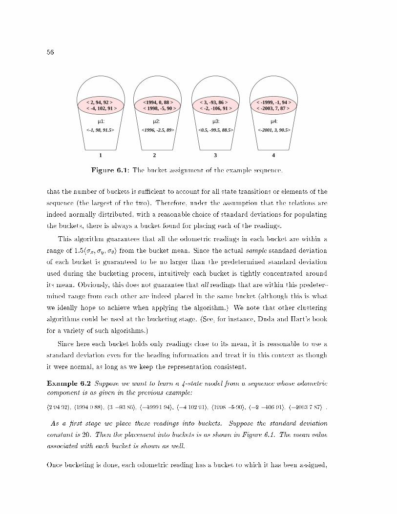
56<-1, 98, 91.5>

µ1:

1

µ2:

<1996, -2.5, 89>

2

µ3:

<0.5, -99.5, 88.5>

3

µ4:

<-2001, 3, 90.5>

4

< -4, 102, 91 >< 2, 94, 92 > <1994, 0, 88 >

< 1998, -5, 90 > < -2, -106, 91 >< 3, -93, 86 > < -1999, -1, 94 >

< -2003, 7, 87 >Figure 6.1: The bu ket assignment of the example sequen e.that the number of bu kets is suÆ ient to a ount for all state transitions or elements of thesequen e (the largest of the two). Therefore, under the assumption that the relations areindeed normally distributed, with a reasonable hoi e of standard deviations for populatingthe bu kets, there is always a bu ket found for pla ing ea h of the readings.This algorithm guarantees that all the odometri readings in ea h bu ket are within arange of 1:5h�x; �y; ��i from the bu ket mean. Sin e the a tual sample standard deviationof ea h bu ket is guaranteed to be no larger than the predetermined standard deviationused during the bu keting pro ess, intuitively ea h bu ket is tightly on entrated aroundits mean. Obviously, this does not guarantee that all readings that are within this predeter-mined range from ea h other are indeed pla ed in the same bu ket (although this is whatwe ideally hope to a hieve when applying the algorithm.) We note that other lusteringalgorithms ould be used at the bu keting stage. (See, for instan e, Duda and Hart's bookfor a variety of su h algorithms.)Sin e here ea h bu ket holds only readings lose to its mean, it is reasonable to use astandard deviation even for the heading information and treat it in this ontext as thoughit were normal, as long as we keep the representation onsistent.Example 6.2 Suppose we want to learn a 4-state model from a sequen e whose odometri omponent is as given in the previous example:h2 94 92i; h1994 0 88i; h3 �93 86i; h�19991 94i; h�4 102 91i; h1998 �5 90i; h�2 �106 91i; h�2003 7 87i :As a �rst stage we pla e these readings into bu kets. Suppose the standard deviation onstant is 20. Then the pla ement into bu kets is as shown in Figure 6.1. The mean valueasso iated with ea h bu ket is shown as well.On e bu keting is done, ea h odometri reading has a bu ket to whi h it has been assigned,

57and the next phase of the algorithm starts. It onsists of state-tagging ea h odometri reading. Ea h odometri reading, rt, is assigned a pair of states, si; sj , orresponding tothe origin state (from whi h the transition took pla e) and the destination state (to whi hthe transition led), respe tively. In onjun tion with this pro ess the mean entries, �ij , ofthe relation matrix R are populated.Example 6.3 Returning to the sequen e used in example 6.2, the pro ess is demonstratedin Figure 6.2. We assume that the re ording starts at state 0, and that the odometri hange-179.5> 95.5,<1995,

98, 91.5>

<-1,

2.5, -89>

<-1996,

89> -2.5,<1996,

-91.5> -98,< 1,

<-1995, -95.5, 179.5>

<0,0,0>

<0,0,0>

<0,0,0>

<0,0,0>

<0,0,0>

<0,0,0>

<0,0,0>

<0,0,0>

98, 91.5>

<-1, 95.5,<1995,

-179.5>

< 0.5,

88.5> -99.5,

99.5, -88.5>

<-0.5,

177.5>

<1996.5, -102,

102, -177.5>

<-1996.5,

<-1995, -95.5, 179.5>

-98, -91.5>

< 1,

89> -2.5,<1996,

2.5, -89>

<-1996,

4, 91>

<-1995.5,

<0,0,0>

<0,0,0>

<0,0,0>

-4, -91>

<1995.5,<0,0,0>

-91.5>

< 1, -98,

<0,0,0>

<0,0,0>

<0,0,0>

<0,0,0>

98,<-1,

91.5>

Bucket(R[0][1]) = µ1

0 321 3210

1 1

2 2

3

0

3

0

A

S: 0. 1S: 0

B

,..., S:0, 1, 2, 3, 0, 1, 2, 3, 0

S: 0,1,2,3,0

µ4Bucket(R[3][0]) =

Bucket(R[2][3]) = µ3

32103210

0 0

1

2

3

1

2

3

C D

Bucket(R[1][2]) = µ2

S: 0,1,2,3S: 0, 1, 2Figure 6.2: Populating the odometri relation matrix and reating a state tagging se-quen e.through self transitions is 0, with some small standard deviation (we use 20 here as well).

58This is shown on part A of the �gure.Sin e the �rst element in the sequen e, h2 94 92i is more than two standard deviationsaway from the mean �[0℄[0℄ and no other entry in the relation row of state 0 is populated wepi k 1 as the next state and populate the mean �[0℄[1℄ to be the same as the mean of bu ket 1,to whi h h2 94 92i belongs. To maintain geometri al onsisten y the mean �[1℄[0℄ is set to be��[0℄[1℄, as shown in part B of the �gure. We now have 2 non-diagonal entries populated inthe matrix and the state sequen e is h0; 1i. The entry [0℄[1℄ in the matrix be omes asso iatedwith bu ket 1, and this information is kept for helping with tagging future odometri readingswhi h were assigned the same bu ket.The next odometri reading, h1994 0 88i, is also several standard deviations from anypopulated mean in row 1 (where 1 is the urrent believed state) of the relation matrix. Hen e,we pi k a new state 2, and set the mean �[1℄[2℄ to be �2 | the mean of the bu ket 2 |to whi h the odometri reading belongs. For symmetry preservation, �[2℄[1℄ is set to be��[1℄[2℄. We re ord that entry [1℄[2℄ in the matrix be omes asso iated with bu ket 2. Forpreserving additivity we also set �[0℄[2℄ to be the sum of �[0℄[1℄ and �[1℄[2℄. �[2℄[0℄ is setto ��[0℄[2℄. Similarly, �[2℄[3℄ is updated to be the mean of bu ket 3, ausing the setting of�[3℄[2℄, �[1℄[3℄, �[0℄[3℄, �[3℄[1℄, and �[3℄[0℄. Bu ket 3 is asso iated with �[2℄[3℄.At this stage the odometri table is fully populated, as shown in part D of Figure 6.2.Sin e the mean al ulation is based on a umulation, the standard deviations grow as well,as the square root of the a umulated varian es, although this is not shown in the �gure.The state sequen e at this point is: h0; 1; 2; 3i. The next reading, h�1999 �1 94i, iswithin one standard deviation from �[3℄[0℄ and therefore the next state is 0. Entry [3℄[0℄is asso iated with bu ket 4, (the bu ket to whi h the reading was assigned), and the statesequen e be omes: h0; 1; 2; 3; 0i.The next reading, being from bu ket 1 is asso iated with the relation from state 0 thatis tagged by bu ket 1, namely, state 1. By repeating this for the last two readings the �nalstate transition sequen e be omes h0; 1; 2; 3; 0; 1; 2; 3; 0i.Figure 6.3 provides a pseudo- ode version of this algorithm. The input to the algorithm isthe odometri reading sequen e, Eo, of length T�1, together with the bu keting information.For 0 � i � T � 1 , Bu kets[i℄ ontains the number of the bu ket to whi h the ith odometri reading in the sequen e is assigned. The algorithm produ es a sequen e S of the statesbelieved to have been traversed when the data sequen e E was produ ed, as well as aninitial estimate for the mean of ea h entry in the relation matrix R.

59Populate-and-Tag(E0; T; Bu kets)1 for i 0 to n2 do3 �[i℄[i℄ 04 Dev[i℄[i℄ �5 for j 0 to n; j 6= i6 do7 �[i℄[j℄ EMPTY89 S[0℄ 010 Current tag 011 for i 0 to T � 112 do Find j s.t. �[ Current tag ℄[j℄:Bu ket = Bu kets[i℄13 if not found14 then Find j s.t. �[ Current tag ℄[j℄ is within 1.5 standard deviations from Eo[i℄:15 if not found16 then Find j s.t. �[ Current tag ℄[j℄ is still unde�ned17 if found18 then �[ Current tag ℄[j℄ Bu kets[i℄:mean:19 �[ Current tag ℄[j℄:Bu ket Bu kets[i℄20 Propagate update to maintain symmetry and additivity.2122 else Find j s.t. j 6= Current tag23 and �[ Current tag ℄[j℄ is losest to Eo[i℄:242526 Current tag = j:27 S[i + 1℄ = j:2829 return S Figure 6.3: The state tagging algorithm.

60 It is possible that by the end of the tagging algorithm, some rows or olumns of therelation matrix are still unpopulated. This happens when there is too little data to learnfrom or when the number of states provided to the algorithm is too large with respe t to thea tual model. In su h ases we an either \trim" the model, using the number of populatedrows as the number of states, or pi k random odometri readings to populate the rest ofthe table, improving these estimates later. Note that the �rst approa h suggests a methodfor learning the number of states in the model when this is not given, starting from a grossover-estimate of the number, and trun ating it to the number of populated rows in theodometri table after initialization is performed.On e the state-transition sequen e is obtained, the rest of the algorithm is the sameas before, deriving state-transition ounts from the state-transition sequen e, assigning theobservations to the states under the assumption that the state sequen e is orre t, andobtaining the state-transition and observation statisti s.The omplexity of this algorithm is worst- ase bounded by the omplexity of a singleBaum-Wel h iteration, namely TN2. To roughly estimate its run time, we observe thatthe algorithm has to �nd for ea h of the T � 1 odometri readings in the sequen e Eo, anassignment of a destination state from within N possible assignment and update the rest ofthe odometri relationships that are a�e ted by this assignment. If with ea h assignmentwe would have had to update N2 entries, we would have had a omplexity of TN2. Notethat the relation matrix an only be fully populated on e, hen e altogether the omplexityfor the tagging stage is TN +N2.The preliminary bu keting stage requires an assignment of a bu ket to ea h of theT � 1 odometri readings. We take as the maximal number of bu kets min(N2; T � 1),that is, at most every reading has its own bu ket. In this ase, however, no two readingsre e t the same state-transition. The maximal number of possible distin t state transitionsover N states is N2. Therefore, in any ase, the omplexity of bu keting is bounded bymin(TN2; T 2).Thus, the initialization phase does not in ur mu h overhead on the algorithm, and isequivalent to performing a single additional iteration of the Baum-Wel h pro edure. Judgingby the improvement in the results due to the initialization, it is well justi�ed.

Chapter 7Experiments within a GlobalFrameworkThe goal of the work des ribed so far is to use odometry to improve the learning of topolog-i al models, while using fewer iterations and less data. We tested our algorithm in a simplerobot-navigation world. Our experiments onsist of running the algorithm both on dataobtained from a simulated model and on data gathered by our mobile robot, Ramona. Theamount of data gathered by Ramona is used here as a proof of on ept but is not suÆ ientfor statisti al analysis. For the latter, we use data obtained from the simulated model.Signi� ant assumptions underlying all the experiments des ribed in this hapter are thatthe orridors in the environment are all perpendi ular to ea h other, and that the agent |both in the real robot ase and in the simulated ase | is aware of this1. Hen e, after ea hturn the agent assumes that its new heading is almost perpendi ular to its previous heading.This assumption is used when the agent is gathering its data sequen e, E. The assumptionis satis�ed in most oÆ e buildings, but is violated in a lot of other environments. We relaxthe perpendi ularity assumption starting in Chapter 8.7.1 Robot DomainThe robot used in our experiments, Ramona, is a modi�ed RWI B21 robot. It has a ylindri al syn hro-drive base, 24 ultrasoni sensors and 24 infrared sensors, situated evenlyaround its ir umferen e. The infrared sensors are used mostly for short-range obsta le1Thanks to Sebastian Thrun for expli itly expressing this assumption61

62avoidan e. The ultrasoni sensors are longer ranged, and are used for obtaining (noisy)observations of the environment. In the experiments des ribed here, the robot follows apres ribed path through the orridors in the oÆ e environment of our department.Low-level software2 provides a level of abstra tion that allows the robot to move throughhallways from interse tion to interse tion and to turn ninety degrees to the left or right.The software uses sonar data to distinguish doors, openings, and interse tions along thepath, and to stop the robot's urrent a tion whenever su h a landmark is dete ted. Ea hstop | either due to the natural termination of an a tion or due to a landmark dete tion| is onsidered by the robot to be a \state".At ea h stop, ultrasoni data interpretation allows the robot to per eive, in ea h of thethree ardinal dire tions, (front, left and right), whether there is an open spa e, a door, awall, or something unknown.The robot also has en oders on its wheels that allow it to estimate its pose (positionand orientation) with respe t to its pose at the previous interse tion. After re ording boththe sonar-based observations and the odometri information, the robot goes on to exe utethe following pres ribed a tion. The next a tion ommand is issued manually by a humanbeing. Of ourse, both the a tion and per eption routines are subje t to error. The pathRamona followed onsists of 4 onne ted orridors in our building, whi h in lude 17 states,as shown in Figure 7.1.In our simulation, we manually generated an hmm representing a pres ribed path of therobot through the omplete oÆ e environment of our department, onsisting of 44 states,and the asso iated transition, observation, and odometri distributions. The transitionprobabilities re e t a tion failure rate of about 5� 10%. That is, the probability of movingfrom the urrent state to the orre t next state in the environment, under the predetermineda tion is between 0:85 and 0:95. The probability of self transition is typi ally between 0:05and 0:15. Some small probability (typi ally smaller than 0:02) is sometimes assigned toother transitions. Our experien e with the real robot proves that this is a reasonabletransition model, sin e typi ally the robot moves to the next state orre tly, and the onlyerror that o urs with some signi� ant frequen y is when it does not move at all, dueto sonar interpretation indi ating a barrier when there is a tually none. On e the a tion ommand is repeated the robot usually performs the a tion orre tly, moving to the expe tednext state. The observation distribution typi ally assign probabilities of 0:85� 0:95 to thetrue observation that should be per eived by the robot at ea h state, and probabilities of2The low-level software was written by James Kurien.

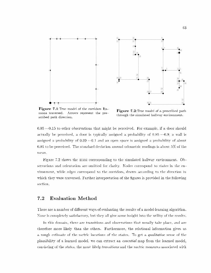
630

1

2

3 4 5 6 7 8

9

10

11

12

13141516

0

12345

6

8

91012

13

14 15 17 24

25

26 27 2829

7 4243

18

19

202122

23

11

30 31 3233

34

353638

41

37

39

40

16Figure 7.1:True model of the orridors Ra-mona traversed. Arrows represent the pre-s ribed path dire tion. Figure 7.2:True model of a pres ribed paththrough the simulated hallway environment.0:05� 0:15 to other observations that might be per eived. For example, if a door shoulda tually be per eived, a door is typi ally assigned a probability of 0:85 � 0:9, a wall isassigned a probability of 0:09 � 0:1 and an open spa e is assigned a probability of about0:01 to be per eived. The standard deviation around odometri readings is about 5% of themean.Figure 7.2 shows the hmm orresponding to the simulated hallway environment. Ob-servations and orientation are omitted for larity. Nodes orrespond to states in the en-vironment, while edges orrespond to the orridors, drawn a ording to the dire tion inwhi h they were traversed. Further interpretation of the �gures is provided in the followingse tion.7.2 Evaluation MethodThere are a number of di�erent ways of evaluating the results of a model-learning algorithm.None is ompletely satisfa tory, but they all give some insight into the utility of the results.In this domain, there are transitions and observations that usually take pla e, and aretherefore more likely than the others. Furthermore, the relational information gives usa rough estimate of the metri lo ations of the states. To get a qualitative sense of theplausibility of a learned model, we an extra t an essential map from the learned model, onsisting of the states, the most likely transitions and the metri measures asso iated with

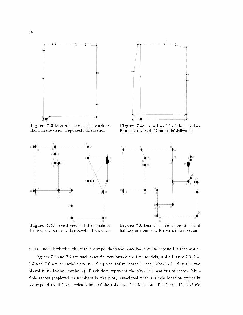
640

15

16

1

2

3 4 5 6 7 8

9

10

11

12

1314

3 4 5 6 7 8

9

10

11

12

1314

015

16

1

2

12

9

2

117 14 46

15

1

516

10

0

813

3

12

916

13

3

12

7 11 14 4

6

10

15

0

8

1

5

2

Figure 7.3:Learned model of the orridorsRamona traversed. Tag-based initialization. Figure 7.4:Learned model of the orridorsRamona traversed. K-means initialization.0

1234

5

6

13141516

28

19

30 35

36

37

38

3940 41

42

43

10

17

7 89

1812

27

29

31

2324

25

26

32

33

34

20

21

22

11

23

02

36

28

1312740

6

3229 22

31

20

4330 42

10

11 8

25

19

393815

21

24

3

427

349

26

16

33

35

17

14

51

37Figure 7.5:Learned model of the simulatedhallway environment. Tag-based initialization. Figure 7.6:Learned model of the simulatedhallway environment. K-means initialization.them, and ask whether this map orresponds to the essentialmap underlying the true world.Figures 7.1 and 7.2 are su h essential versions of the true models, while Figure 7.3, 7.4,7.5 and 7.6 are essential versions of representative learned ones, (obtained using the twobiased initialization methods). Bla k dots represent the physi al lo ations of states. Mul-tiple states (depi ted as numbers in the plot) asso iated with a single lo ation typi ally orrespond to di�erent orientations of the robot at that lo ation. The larger bla k ir le

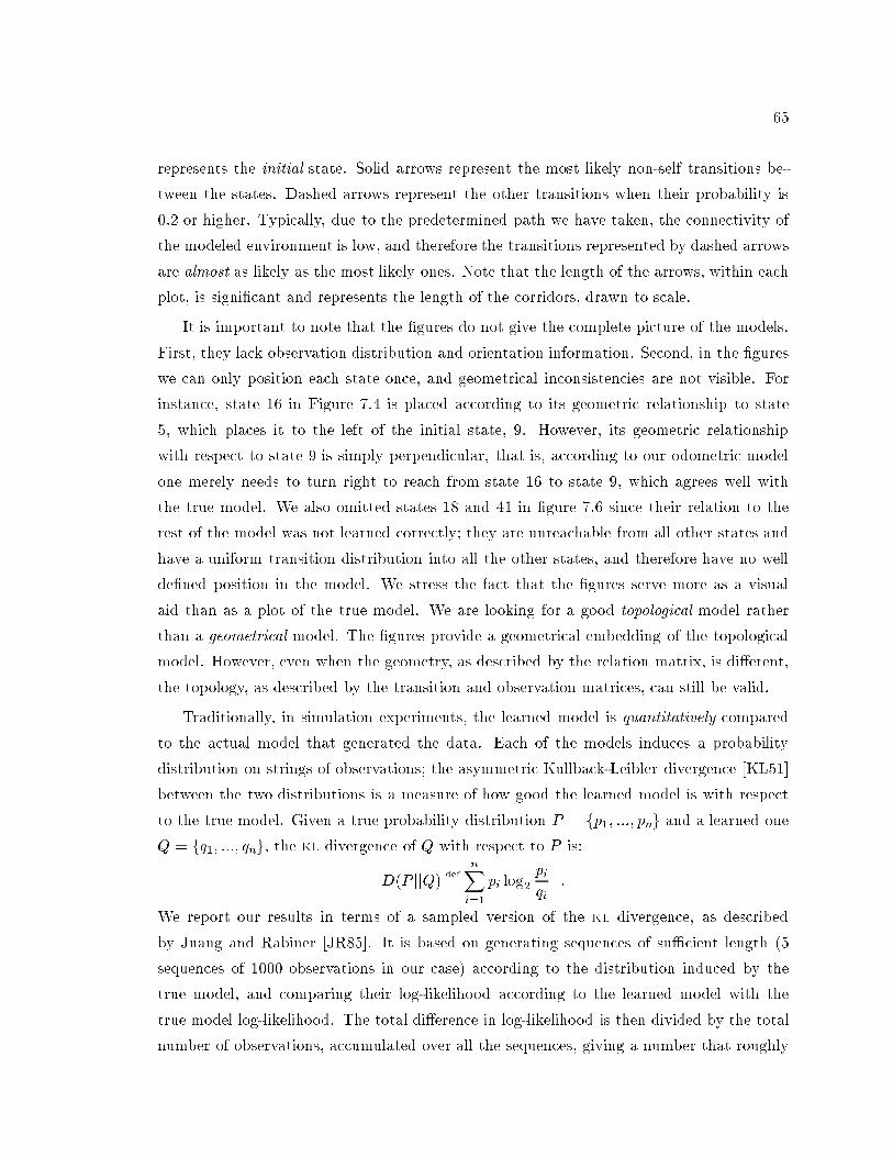
65represents the initial state. Solid arrows represent the most likely non-self transitions be-tween the states. Dashed arrows represent the other transitions when their probability is0:2 or higher. Typi ally, due to the predetermined path we have taken, the onne tivity ofthe modeled environment is low, and therefore the transitions represented by dashed arrowsare almost as likely as the most likely ones. Note that the length of the arrows, within ea hplot, is signi� ant and represents the length of the orridors, drawn to s ale.It is important to note that the �gures do not give the omplete pi ture of the models.First, they la k observation distribution and orientation information. Se ond, in the �gureswe an only position ea h state on e, and geometri al in onsisten ies are not visible. Forinstan e, state 16 in Figure 7.4 is pla ed a ording to its geometri relationship to state5, whi h pla es it to the left of the initial state, 9. However, its geometri relationshipwith respe t to state 9 is simply perpendi ular, that is, a ording to our odometri modelone merely needs to turn right to rea h from state 16 to state 9, whi h agrees well withthe true model. We also omitted states 18 and 41 in �gure 7.6 sin e their relation to therest of the model was not learned orre tly; they are unrea hable from all other states andhave a uniform transition distribution into all the other states, and therefore have no wellde�ned position in the model. We stress the fa t that the �gures serve more as a visualaid than as a plot of the true model. We are looking for a good topologi al model ratherthan a geometri al model. The �gures provide a geometri al embedding of the topologi almodel. However, even when the geometry, as des ribed by the relation matrix, is di�erent,the topology, as des ribed by the transition and observation matri es, an still be valid.Traditionally, in simulation experiments, the learned model is quantitatively omparedto the a tual model that generated the data. Ea h of the models indu es a probabilitydistribution on strings of observations; the asymmetri Kullba k-Leibler divergen e [KL51℄between the two distributions is a measure of how good the learned model is with respe tto the true model. Given a true probability distribution P = fp1; :::; png and a learned oneQ = fq1; :::; qng, the kl divergen e of Q with respe t to P is:D(P jjQ) def= nXi=1 pi log2 piqi :We report our results in terms of a sampled version of the kl divergen e, as des ribedby Juang and Rabiner [JR85℄. It is based on generating sequen es of suÆ ient length (5sequen es of 1000 observations in our ase) a ording to the distribution indu ed by thetrue model, and omparing their log-likelihood a ording to the learned model with thetrue model log-likelihood. The total di�eren e in log-likelihood is then divided by the totalnumber of observations, a umulated over all the sequen es, giving a number that roughly

66200 400 600 800 1000

200

400

600

800

1000

1200

-1500 -1250 -1000 -750 -500 -250

-1500

-1000

-500

500

1000

Figure 7.7:A data sequen e gathered by Ra-mona. Figure 7.8:A data sequen e generated by oursimulator.measures the di�eren e in log-likelihood per observation. Formally stated, let M1 be thetrue model and M2 a learned one. By generating K sequen es S1; : : : ; SK, ea h of lengthT , from the true model, M1, the sampled kl-divergen e, Ds is:Ds(M1jjM2) = KXi=1[log(Pr(SijM1))� log(Pr(SijM2))℄KT :We ignore the odometri information when applying the kl measure, thus allowing om-parison between purely topologi al models that are learned with and without odometry.7.3 ResultsWe let Ramona go around the path depi ted in Figure 7.1 and olle t a sequen e of about300 observations. Figure 7.7 plots the sequen e of metri oordinates, proje ted on hx; yi,obtained by a umulating onse utive odometri readings (as des ribed in Se tion 6.1). Weapplied the learning algorithm to the data 30 times. 10 of these runs were started froma k-means-based initial model, 10 started from a tag-based initial model, and 10 startedfrom a random initial model. In addition we also ran the standard Baum-Wel h algorithm,ignoring the odometri information, 10 times. (Note that there is non-determinism evenwhen using biased initial models, sin e the k-means lustering starts from random seeds,and low random noise is added to the data in all algorithms to avoid numeri al instabilities,thus multiple runs give multiple results).

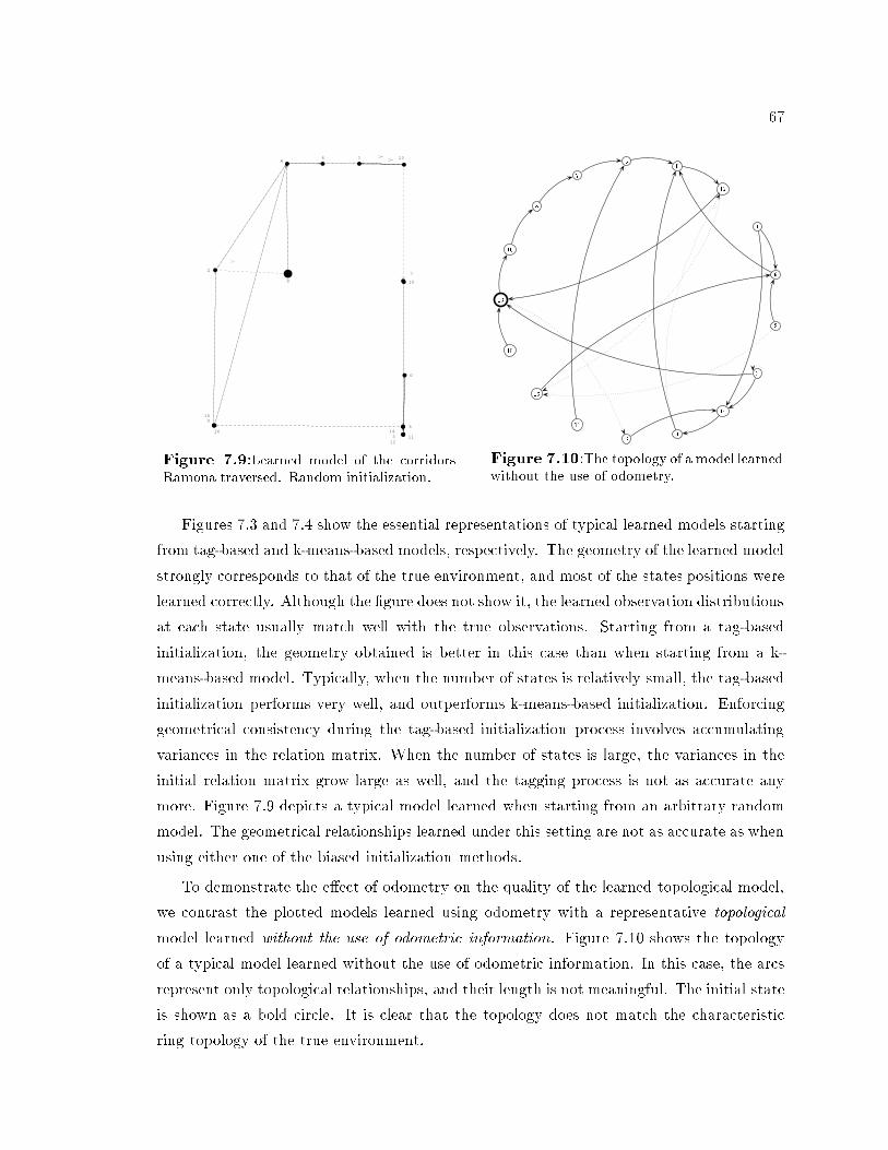
678

46 131

10

516

9

2

0

11

15

143

7

12

16 10 8 7 5 0 12 1 9231446111315Figure 7.9:Learned model of the orridorsRamona traversed. Random initialization. Figure 7.10:The topology of a model learnedwithout the use of odometry.Figures 7.3 and 7.4 show the essential representations of typi al learned models startingfrom tag-based and k-means-based models, respe tively. The geometry of the learned modelstrongly orresponds to that of the true environment, and most of the states positions werelearned orre tly. Although the �gure does not show it, the learned observation distributionsat ea h state usually mat h well with the true observations. Starting from a tag-basedinitialization, the geometry obtained is better in this ase than when starting from a k-means-based model. Typi ally, when the number of states is relatively small, the tag-basedinitialization performs very well, and outperforms k-means-based initialization. Enfor inggeometri al onsisten y during the tag-based initialization pro ess involves a umulatingvarian es in the relation matrix. When the number of states is large, the varian es in theinitial relation matrix grow large as well, and the tagging pro ess is not as a urate anymore. Figure 7.9 depi ts a typi al model learned when starting from an arbitrary randommodel. The geometri al relationships learned under this setting are not as a urate as whenusing either one of the biased initialization methods.To demonstrate the e�e t of odometry on the quality of the learned topologi al model,we ontrast the plotted models learned using odometry with a representative topologi almodel learned without the use of odometri information. Figure 7.10 shows the topologyof a typi al model learned without the use of odometri information. In this ase, the ar srepresent only topologi al relationships, and their length is not meaningful. The initial stateis shown as a bold ir le. It is lear that the topology does not mat h the hara teristi ring topology of the true environment.

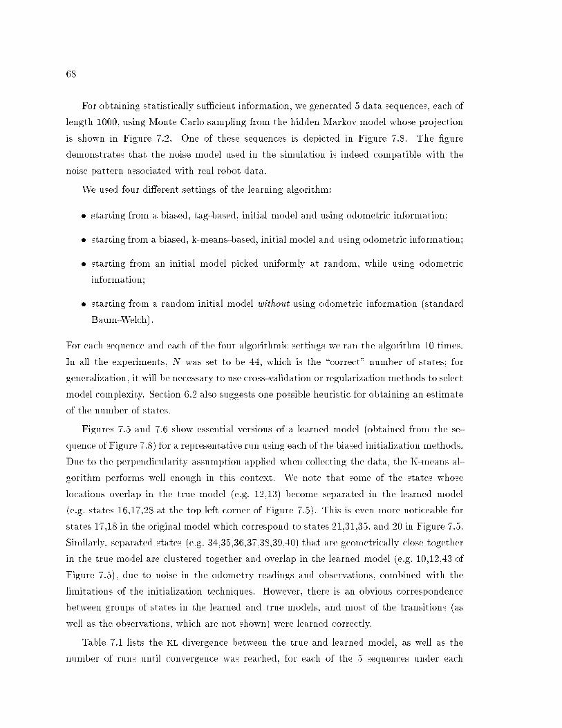
68 For obtaining statisti ally suÆ ient information, we generated 5 data sequen es, ea h oflength 1000, using Monte Carlo sampling from the hidden Markov model whose proje tionis shown in Figure 7.2. One of these sequen es is depi ted in Figure 7.8. The �guredemonstrates that the noise model used in the simulation is indeed ompatible with thenoise pattern asso iated with real robot data.We used four di�erent settings of the learning algorithm:� starting from a biased, tag-based, initial model and using odometri information;� starting from a biased, k-means-based, initial model and using odometri information;� starting from an initial model pi ked uniformly at random, while using odometri information;� starting from a random initial model without using odometri information (standardBaum-Wel h).For ea h sequen e and ea h of the four algorithmi settings we ran the algorithm 10 times.In all the experiments, N was set to be 44, whi h is the \ orre t" number of states; forgeneralization, it will be ne essary to use ross-validation or regularization methods to sele tmodel omplexity. Se tion 6.2 also suggests one possible heuristi for obtaining an estimateof the number of states.Figures 7.5 and 7.6 show essential versions of a learned model (obtained from the se-quen e of Figure 7.8) for a representative run using ea h of the biased initialization methods.Due to the perpendi ularity assumption applied when olle ting the data, the K-means al-gorithm performs well enough in this ontext. We note that some of the states whoselo ations overlap in the true model (e.g. 12,13) be ome separated in the learned model(e.g. states 16,17,28 at the top left orner of Figure 7.5). This is even more noti eable forstates 17,18 in the original model whi h orrespond to states 21,31,35, and 20 in Figure 7.5.Similarly, separated states (e.g. 34,35,36,37,38,39,40) that are geometri ally lose togetherin the true model are lustered together and overlap in the learned model (e.g. 10,12,43 ofFigure 7.5), due to noise in the odometry readings and observations, ombined with thelimitations of the initialization te hniques. However, there is an obvious orresponden ebetween groups of states in the learned and true models, and most of the transitions (aswell as the observations, whi h are not shown) were learned orre tly.Table 7.1 lists the kl divergen e between the true and learned model, as well as thenumber of runs until onvergen e was rea hed, for ea h of the 5 sequen es under ea h

69Seq. Tag-based k-means Random No Odo# kl Iter.# kl Iter. # kl Iter. # kl Iter. #1 1.027 23.7 1.023 30.0 0.954 23.4 6.351 124.12 1.006 41.3 0.994 31.4 0.953 25.8 4.863 126.03 0.984 16.9 1.029 21.9 1.035 26.6 5.927 113.04 1.124 15.8 1.021 25.9 1.017 23.6 6.261 107.45 1.029 8.8 1.142 27.2 1.035 32.4 4.802 122.9Table 7.1: Average results of four learning settings with �ve training sequen es.of the 4 learning settings, averaged over 10 runs per sequen e. We stress that ea h kldivergen e measure is al ulated based on new data sequen es that are generated from thetrue model, as des ribed in Se tion 7.2. The 5 sequen es from whi h the models were learneddo not parti ipate in the testing pro ess. From the table it is lear that the kl divergen ewith respe t to the true model for models learned using odometry, starting from either abiased or a random initial model, is about 5 times smaller than for models learned withoutodometry data. The standard deviation around the KL-divergen e means was about 1.5 forthe no-odometry setting and about 0.1 (often lower) for the odometri settings. To he kthe signi� an e of our results we used the simple two-sample t-test. The models learnedusing odometri information have statisti ally signi� antly (p � 0:9995) lower average kldivergen e than the others.The models learned using random initialization seem slightly better in terms of the klmeasure than the ones learned with biased initialization and this di�eren e is statisti allysigni� ant. A lose look at the obtained models reveals that the models based on biasedinitialization are more peaked (that is, have more probabilities very lose to 0 and to 1)than the ones based on random initialization3 . Sin e the true model is slightly less peakedthan the ones learned using biased initialization, it o asionally generates, when we exe utethe kl routine, sequen es that are quite unlikely a ording to its own distribution andhighly unlikely a ording to the learned model distribution. This results in a larger kl-divergen e for the models learned from biased initialization with respe t to the true model.To avoid this di�eren e in peakedness it might be desirable, during the learning stage, touse the Bayesian approa h, biasing the learning pro ess towards models that do not haveas sharp a distribution over transitions and observations. This will ensure that the modelswould a ommodate even the least likely events in the true environment. It is also possibleto post-pro ess learned models, adding a �xed small onstant to near-0 probabilities and3The relative atness of odometri models learned from a random starting point was dis ussed in Chap-ter 6.

70subtra ting a small onstant from near-1 probabilities.The number of iterations required for onvergen e when learning using odometri infor-mation is roughly 1=4 of that required when ignoring su h information. Again, the t-testveri�es the signi� an e (p > 0:9995) of this result. The standard deviation around themean iteration number is about 10 for models learned from biased initial points (lower thanthat when the number of iterations is low and higher than that when the number of itera-tions is high). In the ase of random initialization the standard deviation is also typi allyaround 10. When no odometri information is used the standard deviation is about 30. Thenumber of iterations is statisti ally signi� antly lower (p > 0:95) when using the tag-basedinitialization than when using any other initialization strategy.It is important to point out that the number of iterations, although mu h lower, doesnot automati ally imply that the algorithm works faster or runs in less time. The majorbottlene k is the fa t that we need to al ulate within the forward-ba kward al ulations,as des ribed in Se tion 4.2.1, the values of the normal and the von-Mises densities. Theserequire the al ulation of exponent terms rather than simple multipli ations, slowing downthe runs onsiderably, under the urrent na��ve implementation. However, we an solve thisby augmenting the program with look-up tables for obtaining the relevant values ratherthan al ulating them. In addition, we an take advantage of the symmetry in the relationstable to ut down on the amount of al ulation required. It is also possible to use the fa tthat many odometri relations remain un hanged (parti ularly in the later iterations of thealgorithm) from one iteration to the next, and therefore values an be a hed and sharedbetween iterations rather than be re al ulated at ea h iteration.The initial lustering strongly biases the out ome of learning; it is important to un-derstand whether this bias is useful. When the entire model is initialized at random, theresulting models are usually lose, in terms of the kl-divergen e, to the true model. This isdue to two fa tors; �rst, by being typi ally atter than the other models, they give reason-able likelihood to any data sequen e, and se ond, by starting from an odometri model thatis typi ally bad with respe t to the data, the algorithm ends up not learning mu h of thegeometri setting of the environment. Therefore it an learn topologies that may a ountfor the probabilisti distribution of the data but do not agree with the true topology. Thisis demonstrated in more detail in Se tion 11.3.When starting from a tag-based initial model, the number of iterations is typi allylower than when using any other setting. The models obtained when starting either from a

71Seq. Tag-based k-means Random No Odolength Mean Std. Mean Std. Mean Std. Mean Std.KL Dev. KL Dev. KL Dev. KL Dev.1000 0.984 0.049 1.029 0.111 1.035 0.063 5.927 1.956900 1.173 0.351 1.176 0.162 1.027 0.077 7.852 1.446800 1.108 0.094 1.220 0.102 1.068 0.045 9.624 1.755700 1.185 0.160 1.329 0.111 1.116 0.104 10.504 2.774600 1.346 0.249 2.575 1.922 1.250 0.237 14.576 3.498500 1.205 0.066 2.049 0.717 1.270 0.137 19.649 4.975400 1.279 0.050 2.558 1.827 1.285 0.214 26.341 4.357300 1.737 0.428 2.447 0.369 1.599 0.508 33.252 4.444200 14.047 11.635 2.781 0.406 3.946 2.704 52.780 4.147100 63.438 1.482 20.606 10.807 12.770 11.987 78.982 6.394Table 7.2: Average results of three learning settings with 10 in rementally longer se-quen es.k-means based or from a tag-based initialization are about equivalent in quality, both topo-logi ally and geometri ally. However, sin e the tag-based algorithm is almost deterministi the results obtained by using it are more onsistent, and are less prone to hange due tovarying initial onditions. Typi ally, when the initialization is good, most of the work is al-ready done and the em algorithm qui kly �lls in the details. However, if the initial k-means lustering is bad, it is often lose to a poor lo al maximum and the algorithm is unable toadjust it well. It may be best to run the algorithm multiple times, taking the model withthe highest likelihood as the �nal result.To examine the in uen e of the amount of data on the quality of the learned models,we took one of the 5 sequen es (Seq. #3) and used its pre�xes of length 100 to 1000 (the omplete sequen e), in in rements of 100, as individual sequen es. We ran ea h of the fouralgorithmi settings over ea h of the 10 pre�x sequen es, 10 times repeatedly. We then usedthe kl-divergen e as des ribed above to evaluate ea h of the resulting models with respe tto the true model. For ea h pre�x length we averaged the kl-divergen e over the 10 runs.Table 7.2 summarizes the results of this experiment. It lists the mean kl-divergen eover the 10 runs for ea h of the pre�xes, as well as the standard deviation around this mean.The plot in Figure 7.11 depi ts the kl-divergen e as a fun tion of the sequen e length forea h of the three settings. Both the table and the plot demonstrate that, in terms of thekl-divergen e, our algorithm, whi h uses odometri information, is robust in the fa e ofdata redu tion. In ontrast, learning without the use of odometry is mu h more sensitiveto redu tion in the amount of data.Again, we applied the two-sample t-test to verify the statisti al signi� an e of these

720 200 400 600 800 1000

Seq. Length

0

10

20

30

40

50

KL

RandomTag-based

K-meansNoOdoFigure 7.11: Average kl-divergen e as a fun tion of the sequen e length.results. For example, the kl-divergen e being greater for models learned from a sequen eof length 800 than from a sequen e of length 1000, without the use of odometry, is highlystatisti ally signi� ant (p > 0:999). In ontrast, the kl-divergen e is usually not highlystatisti ally signi� antly greater when the odometry is used, for either biased or randommodels. The kl-divergen e of the learned biased model u tuates somewhat sin e shortersequen es tend to have less a umulated error on their readings, thus lustering may performbetter, resulting in better learned models despite the fewer data points available (see forinstan e the hange from 600 to 500 observations).We note that the data sequen e is twi e as \wide" when odometry is used than whenit is not; that is, there is more information in ea h element of the sequen e when odometrydata is re orded. However, the e�ort of re ording this additional odometri information isnegligible, and is well rewarded by the fa t that fewer observations and less exploration arerequired for obtaining a data sequen e suÆ ient for adequate learning.

Chapter 8State-Relative Coordinate SystemsThroughout the dis ussion so far, we have assumed that there is a single global oordinatesystem within whi h the robot operates. Moreover, we assumed that the robot olle tsits data within a perpendi ular orridor framework and that it is taking advantage of thisperpendi ularity and the single framework while re ording odometri information. Thisassumption an be troublesome in pra ti e. This hapter dis usses the potential prob-lems, and presents our way for relaxing the assumption and addressing the problems. Ademonstration of the e�e tiveness of our solution is presented in Chapter 9.8.1 MotivationWe tend to think about an environment as onsisting of landmarks �xed in a global oor-dinate system and orridors or transitions onne ting these landmarks. However, this viewof the environment may be problemati when robots are involved.Con eptually, a robot has two levels in whi h it operates; the abstra t level, in whi h it enters itself through orridors, follows walls and avoids obsta les, and the physi al level inwhi h motors turn the wheels as the robot moves. In the physi al level many ina ura ies an manifest themselves: wheels an be unaligned with ea h other resulting in a drift to theright or to the left, one motor an be slightly faster than another resulting in similar drifts,an obsta le under one of the wheels an ause the robot to rotate around itself slightly, oruneven oors may ause the robot to slip in a ertain dire tion. In addition, the measuringinstrumentation for odometri information may not be a urate in and of itself. At theabstra t level, orre tive a tions are onstantly exe uted to over ome the physi al drift anddrag. For example, if the left wheel is misaligned and drags the robot leftwards, a orre tive73

74- recorded position- actual position

ε−εFigure 8.1: A robot moving along the solid arrow, while orre ting for drift in the dire tionof the dashed arrow. The dotted arrow marks its re orded hange in position.a tion of moving to the right is onstantly taken in the higher level to keep the robot awayfrom the left wall and entered in the orridor.The phenomena des ribed above have a signi� ant e�e t on the odometry re orded bythe robot, if it is interpreted with respe t to one global framework. For example, onsiderthe robot depi ted in Figure 8.1. It drifts to the left ��Æ when moving from one state to thenext, and orre ts for it by moving �Æ to the right in order to maintain itself entered in the orridor. Let us assume that states are 5 meters apart along the enter of the orridor, andthat the enter of the orridor is aligned with the y axis of the global oordinate system.The robot steps ba k and forth in the orridor from one state to the next. Whenever therobot rea hes a state, its odometry reading hanges by hx; y; �i along the hX; Y; heading idimensions, respe tively. As the robot pro eeds, the deviation with respe t to the x axisbe omes more and more severe. Thus, after going through several transitions, the odometri hanges re orded between every pair of states, if taken with respe t to a global oordinatesystem, be ome larger and larger (espe ially along the X dimension). Similar problems ofin onsistent odometri hanges re orded between pairs of states an arise along any of theodometri dimensions. It is espe ially severe when su h in onsisten ies arise with respe t tothe heading, sin e this an lead to mistakenly swit hing movement along the X and the Yaxes, as well as onfusion between forwards and ba kwards movement (when the deviationin the heading is around 90Æ or 180Æ respe tively). Figure 8.2 demonstrates Ramona's viewof a path through the perfe tly perpendi ular department orridors, depi ted in Figure 7.1,based on its odometri re ording, with respe t to a global oordinate system.A solution to su h a situation is to model the odometri relations of moving from statesi to state sj using a hanging oordinate system whi h is relative to state si, as opposed toa global oordinate system an hored at the initial state. This way, the learned relationship

75200 400 600 800 1000

500

1000

1500

2000

Figure 8.2: A path in a perpendi ular environment plotted based on odometri readingstaken by Ramona.between ea h pair of states, hsi; sji, is reliable despite the fa t that it is based on multi-ple transitions re orded from si to sj . Within the global oordinate system the relationsre orded may vary greatly between one transition from si to the next. We formalize thisidea and provide the update rules for the odometri information based on this approa h inthe rest of this hapter.8.2 Learning Odometri Relations with Relative CoordinatesAs before, our experien e sequen e, E, onsists of T pairs hrt; Vti of re orded odometri rela-tions and observation ve tors. The odometri relations are re orded as before, with respe tto the robot's global oordinate system. However, when learning the relation matrix fromthe odometri readings, we interpret the entry Ri;j in the relation matrix R as en odingthe information with respe t to a oordinate system whose origin is an hored at the statesi; the y axis is aligned with the robot's urrent heading and the x axis is perpendi ular toit. This is depi ted in �gure 8.3. The robot is in state si fa ing in the dire tion pointedto by the y axis, and its relationship to the state sj is des ribed in terms of the oordinatesystem shown in the �gure.To support this interpretation of the relation matrix we need to revisit the formulationof the geometri al- onsisten y onstraints stated in Se tion 3.2, as well as the initializationpro edure and the update formulae used when learning the model.

76x∆

y∆

∆θSi

Sj

y

xFigure 8.3: The robot is in state Si fa ing in the dire tion of the y axis; the relationbetween Si and Sj is measured a ording to Si's oordinate framework.8.2.1 Geometri al Consisten y in a Relative FrameworkThe onsisten y onstraints have to re e t the oordinate system with respe t to whi h theodometry is represented. Note that the hange in heading from one state to the next isindependent of any spe i� oordinate system. Hen e, only the onstraints over the x andy omponents of the odometri relation need to be rede�ned.Given a pair of states a and b, we denote by �hx;yi(a; b) the ve tor h�(Ra;b[x℄); �(Ra;b[y℄)i.Let us de�ne Tab to be the transformation that maps an hxa; yai pair represented withrespe t to the oordinate system of state a, to the same pair represented with respe t tothe oordinate system of state b, hxb; ybi (note that Tab = T �1ba , and ��(a; b) = ���(b; a)).More expli itly, as before, let ��(a; b) be the mean hange in heading from state a tostate b. Then the transformation Tab is de�ned as follows:* xbyb + = Tab* xaya + = * xa os(��(a; b))� ya sin(��(a; b))xa sin(��(a; b)) + ya os(��(a; b)) + :Tab an also be expressed using the matrix notation:Tab = 24 os(��(a; b)) � sin(��(a; b))sin(��(a; b)) os(��(a; b)) 35 :

77We an now rede�ne the onsisten y onstraints given in Se tion 3.2, for the x and y omponents of the odometri relation:� �hx;yi(a; a) = h0; 0i;� �hx;yi(a; b) = �Tba[�hx;yi(b; a)℄ (anti-symmetry);� �hx;yi(a; ) = �hx;yi(a; b) + Tba[�hx;yi(b; )℄ (additivity) :8.2.2 InitializationRe all that the tag-based initialization algorithm, des ribed in Se tion 6.2, maintains ge-ometri al onsisten y while populating the relation matrix. When the matrix representsrelations in a relative oordinate system, the above onstraints need to be taken into a - ount when maintaining the onsisten y of the data. Expli itly, when �ij is set to hx; y; �i,�ji is set to h�(x os(�)� y sin(�)); �(x sin(�) + y os(�)); ��i :Similarly, if �ik is already set to hx1; y1; �1i and �kj is being set to hx2; y2; �2i then �ijneeds to be set tohx1 + (x2 os(�1) + y2 sin(�1)); y1 � (x2 sin(�1)� y2 os(�1)); �1 + �2ii :8.2.3 ReestimationThe reestimation formulae for all the parameters ex ept for the x and y omponents of therelation matrix R, remain as before. However, the reestimation formulae for the x and yparameters are hanged to re e t the relative oordinate systems used. We follow a similarpro ess to the one used when deriving the reestimation formulae in Se tion 4.3.3. Again,we are looking to improve expression 4.21 whi h we repeat here for the sake of larity:Q(R;R) = N�1Xi=0 DXm=1Qmii (R;R) + N�1Xi=0 N�1Xj=(i+1) DXm=1[Qmij (R;R) + Qmji(R;R)℄ ;only this time the symmetry onstraints are:�xji = � os(��ij)�xij + sin(��ij)�yij ; (8.1)�yji = � sin(��ij)�xij � os(��ij)�yij : (8.2)By substituting these expressions for �xji and �yji, taking the derivatives of equation 4.21with respe t to �xij and �yij , equating them to 0, and using the \lag-behind" poli y with

78respe t to the update of standard deviations, as des ribed in Se tion 4.2.2, we obtain thefollowing pair of equations:av1 � u os(�)v2 � w sin(�)v3� �xi;j � lv1 + k( os(�))2v2 + k(sin(�))2v3 �+ �yi;jk os(�) sin(�)� 1v2 � 1v3� = 0 ; (8.3)bv4 + u sin(�)v2 � w os(�)v3+ �xi;jk os(�) sin(�)� 1v2 � 1v3�� �yi;j � lv4 + k(sin(�))2v2 + k( os(�))2v3 � = 0 ; (8.4)wherea =Xt �tijrxt ; b =Xt �tijryt ; u =Xt �tjirxt ; w =Xt �tjiryt ; l =Xt �tij ; k =Xt �tji; v1 = (�xij)2;v2 = (�xji)2; v3 = (�yji)2; v4 = (�yij)2; and � = ��ij :The expressions for �xij and �yij that solve this set of equations onstitute the updateformulae in the x and y dimensions. As before, these update formulae are guaranteed toimprove Q, and are therefore an instan e of the generalized em algorithm.Note that in earlier work [SK98℄ we used an update heuristi of assuming that allvarian es are the same when updating the means, obtaining the following reestimationformulae:�xi;j = T�2Xt=0 (�t(i; j)rt[x℄)� T�2Xt=0 (�t(j; i) h os(��i;j); sin(��i;j)i 24 rt[x℄rt[y℄ 35T�2Xt=0 [�t(i; j) + �t(j; i)℄ ;�yi;j = T�2Xt=0 (�t(i; j)rt[y℄)� T�2Xt=0 (�t(j; i) h� sin(��i;j); os(��i;j)i24 rt[x℄rt[y℄ 35T�2Xt=0 [�t(i; j) + �t(j; i)℄ :These reestimation rules are easily obtained from the more general ones by setting v1; v2; v3; v4to all be the same.This hapter has introdu ed an approa h for learning models from data that is orruptedby umulative rotational error. To demonstrate the e�e tiveness of this approa h we ranexperiments on data that was olle ted without applying the perpendi ularity assumption,thus indeed su�ers from the phenomena des ribed in the beginning of this hapter. Theexperiments and their results are presented in the next hapter.

Chapter 9Experiments Using RelativeCoordinatesSimilar to the experiments presented in Chapter 7, we test our algorithm in a simple robot-navigation world. Again, we use both real robot data and data obtained from the samesimulated model as before, as shown in Figure 9.2, with two distin tions:� The data is generated without the perpendi ularity assumption. This means that thex and y oordinates are not realigned after ea h turn with the global x and y axes,but rather, re orded as is. This is true for both robot data and simulated data.� The algorithm used for learning the model from the data is as des ribed in Se tion 8.2.9.1 Experimental SettingAs before, we provide qualitative results from applying the algorithm to the data obtainedfrom the robot. For statisti ally evaluating our results we used the sampled Kullba k-Leiblerdivergen e of the distribution indu ed by the learned model with respe t to that indu ed bythe true model. The sampled sequen es a ording to whi h the kl-divergen e is al ulatedare generated and ompared as before, ignoring the odometri data.Figure 9.1 depi ts the dire ted path through whi h Ramona moved. This is the sametrue environment as the one des ribed in Chapter 7. Figure 9.3 shows the proje tion of theodometri readings that Ramona re orded along the x and y dimensions, while traversingthis environment. For obtaining statisti ally suÆ ient information, we generated 5 datasequen es, ea h of length 800, using Monte Carlo sampling from the hidden Markov model79

800

1

2

3 4 5 6 7 8

9

10

11

12

13141516

0

12345

6

8

91012

13

14 15 17 24

25

26 27 2829

7 4243

18

19

202122

23

11

30 31 3233

34

353638

41

37

39

40

16Figure 9.1:True model of the orridors Ra-mona traversed. Arrows represent the pre-s ribed path dire tion. Figure 9.2:True model of a pres ribed paththrough the simulated hallway environment.whose proje tion is shown in Figure 9.2. One of these sequen es is depi ted in Figure 9.4.The �gures of both real and simulated data demonstrate that in addition to the noise alongthe x and y measurements, a umulative rotational error is present on e the perpendi ularityassumption is dropped.We use the same four settings of the learning algorithm as before:� starting from a biased, tag-based, initial model and using odometri information;� starting from a biased, k-means based, initial model and using odometri information;� starting from a random initial model and using odometri information;� starting from a random initial model without using odometri information (standardBaum-Wel h).For ea h sequen e and ea h of the four algorithmi settings we ran the algorithm repeatedly10 times. In all the experiments based on simulated data, N was set to be 44, while in theexperiments using real robot data the number of states was set to 17. In both ases thisnumber of states is the \ orre t" one.

81-2500 -2000 -1500 -1000 -500 500 1000

500

1000

1500

2000

2500

3000

-1500 -1000 -500 500

-1500

-1000

-500

500

1000

1500

Figure 9.3:A data sequen e olle ted by Ra-mona in a perpendi ular hallway environment. Figure 9.4:A data sequen e generated by oursimulator, without perpendi ularity assump-tion.9.2 ResultsFigure 9.5 depi ts a typi al model learned from data obtained by the robot, using odometry,starting from a tag-based initial model. The models learned using k-means initializationand uninformed initialization do not typi ally re e t the lear re tangular geometry of thetrue environment, and hen e are not satisfa tory geometri ally. Note that the k-meansinitialization, as des ribed in Se tion 6.1, was expe ted not to perform well in the presen eof umulative rotational error.As before, the geometri al plot used in Figure 9.5 prevents us from observing the ge-ometri al in onsisten ies in the learned model. For example, State 16, when drawn withrespe t to state 15 is at the same x and y oordinates as state 15, but the heading is perpen-di ular to it, that is, the robot needs to turn to the right in order to move from state 15 tostate 16. However, if we were to draw state 16 with respe t to state 1, it should have beenpla ed very lose to where state 0 is, thus orresponding mu h better to the re tangulargeometry of the true environment. Sin e state 1 was drawn with respe t to state 0 and state16 with respe t to state 15, while la king geometri al onsisten y throughout the model,the geometry is somewhat distorted.We ontrast this model with the one shown in Figure 9.6 whi h is the topologi al layout ofa model learned without the use of odometri information, from the same data sequen e. Itis obvious from the �gure that the hara teristi loop topology of the traversed environmentwas not learnt when odometri information was not used.

820

1

2

34

5

6

7

89

10

11

12

13

1415

16

1 11 8 3 7 0 13 2 41012569141516Figure 9.5:Learned model of the orridorsRamona traversed. Initialization is Tag-based. Figure 9.6:Model learned without the use ofodometri information, from the same data se-quen e.Figures 9.7 and 9.8 depi t the geometri al layout of typi al models learned from thesimulated data, starting from a tag-based initial model. These models are not geometri allygood, although some of the re tangular hara teristi s of the environment are visible. Themodels learned using k-means initialization and uninformed initialization are, obviously,geometri ally worse. The tag-based initialization performs mu h better when the numberof states is small. This an be explained by the fa t that when it populates the initialrelation matrix and tags odometri readings, it he ks the proximity of readings to thetable entries, using standard deviations that are a umulated when onsisten y is enfor ed.The larger the number of states, the bigger the deviation be omes, and the less a uratethe tagging pro ess is. It is an interesting possible resear h dire tion to try and learn wellsmall portions of the environment and then ombine them into a omplete map of theenvironment.Table 9.1 lists the kl divergen e between the true and learned models, and the numberof iterations the algorithm took to onverge, for ea h of the 5 sequen es under ea h of the4 learning settings, averaged over 10 runs per sequen e. The kl divergen e with respe tto the true model for models learned using odometry, starting from either a biased or arandom initial model, is about 8-9 times smaller than for models learned without odometri data. Note that in these experiments learning was done from training sequen es of 800observations rather than 1000. Therefore the kl measure for the non-odometri ase ishigher than that given in Table 7.1. The standard deviation around the means is about0.1 for kl distan es learned with odometry, and about 2.5 for models learned without

83Figure 9.7:Learned model of the simulatedenvironment. Initialization is Tag-based. Figure 9.8:Learned model of the simulatedenvironment. Initialization is Tag-based.Seq. Tag-based k-means Random No Odo# kl Iter.# kl Iter. # kl Iter. # kl Iter. #1 1.540 9.90 0.983 19.80 1.110 27.00 6.919 113.302 1.029 15.10 0.984 24.70 1.065 32.60 9.926 113.103 1.301 26.40 1.236 22.70 1.119 27.10 10.030 102.004 1.028 33.50 1.100 36.00 1.020 36.00 9.539 104.205 1.029 28.30 1.107 25.30 1.060 31.90 12.431 112.50Table 9.1: Average results of the four learning settings with �ve training sequen es.odometry. To he k the signi� an e of our results we again applied the two-sample t-test.The models learned using odometri information have statisti ally signi� antly (p� 0:9995)lower average kl divergen e than the others. We an on lude that despite the umulativerotational error in the odometri data, the topologi al models learned using it are mu hbetter than those learned without any odometri information.We noti e that models learned with random initialization and the ones based on k-meanshave a slightly lower kl-divergen e than the models whose learning used the tag-basedinitialization. The explanation to this is again the fa t that the tag-based initialization,whi h is more rigorous than the others, results in more peaked models, typi ally assigningvery low probabilities to the less likely sequen es of the original model, even when thelearned distributions are similar to the true ones. Thus, the divergen e between the learnedand the true model is larger when this initialization is used than when the other methods,whi h result in atter models, are used.

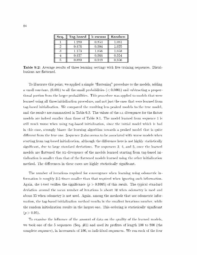
84 Seq. Tag-based k-means Random1 1.280 0.854 1.0812 0.876 0.904 1.0253 1.173 1.056 1.0584 0.837 0.968 0.9545 0.880 0.949 0.956Table 9.2: Average results of three learning settings with �ve training sequen es. Distri-butions are attened.To illustrate this point, we applied a simple \ attening" pro edure to the models, addinga small onstant, (0:001) to all the small probabilities (< 0:0001) and subtra ting a propor-tional portion from the larger probabilities. This pro edure was applied to models that werelearned using all three initialization pro edure, and not just the ones that were learned fromtag-based initialization. We ompared the resulting less peaked models to the true model,and the results are summarized in Table 9.2. The values of the kl-divergen e for the attermodels are indeed smaller than those of Table 9.1. The model learned from sequen e 1 isstill mu h worse when using tag-based initialization, sin e the initial model whi h is badin this ase, strongly biases the learning algorithm towards a peaked model that is quitedi�erent from the true one. Sequen e 3 also seems to be asso iated with worse models whenstarting from tag-based initialization, although the di�eren e here is not highly statisti allysigni� ant, due to large standard deviations. For sequen es 2; 4, and 5, on e the learnedmodels are attened the kl-divergen e of the models learned starting from tag-based ini-tialization is smaller than that of the attened models learned using the other initializationmethod. The di�eren es in these ases are highly statisti ally signi� ant.The number of iterations required for onvergen e when learning using odometri in-formation is roughly 3-5 times smaller than that required when ignoring su h information.Again, the t-test veri�es the signi� an e (p > 0:9995) of this result. The typi al standarddeviation around the mean number of iterations is about 10 when odometry is used andabout 35 when odometry is not used. Again, among the methods that use odometri infor-mation, the tag-based initialization method results in the smallest iterations number, whilethe random initialization results in the largest one. This ordering is statisti ally signi� ant(p > 0:95).To examine the in uen e of the amount of data on the quality of the learned models,we took one of the 5 sequen es (Seq. #1) and used its pre�xes of length 100 to 800 (the omplete sequen e), in in rements of 100, as individual sequen es. We ran ea h of the four

85Seq. Tag-based k-means Random No Odolength Mean Std. Mean Std. Mean Std. Mean Std.KL Dev. KL Dev. KL Dev. KL Dev.800 1.029 0.046 1.107 0.058 1.060 0.105 12.431 2.869700 1.147 0.044 1.102 0.039 1.129 0.080 15.102 3.578600 1.361 0.080 1.276 0.171 1.129 0.142 16.832 2.854500 1.377 0.131 1.267 0.110 1.271 0.118 22.721 4.560400 1.324 0.102 1.216 0.067 1.267 0.085 28.570 4.755300 1.475 0.229 1.930 0.698 2.046 1.024 37.111 6.690200 1.630 0.806 6.493 3.751 3.025 1.776 55.387 3.548100 16.780 8.572 38.722 7.464 11.396 14.796 85.945 4.054Table 9.3: Average results of four learning settings with 8 in rementally longer sequen es.0 200 400 600 800

Seq. Length

0

10

20

30

40

50

KL

RandomK-means

Tag-based

NoOdoFigure 9.9: Average kl-divergen e as a fun tion of the sequen e length.algorithmi settings over ea h of the 8 pre�x sequen es, 10 times repeatedly. We then usedthe kl-divergen e as des ribed above to evaluate ea h of the resulting models with respe tto the true model. For ea h pre�x length we averaged the kl-divergen e over the 10 runs.Table 9.3 summarizes the results of this experiment. It lists the mean kl-divergen eover the 10 runs for ea h of the pre�xes, as well as the standard deviation around this mean.The plot in Figure 9.9 depi ts the kl-divergen e as a fun tion of the sequen e length forea h of the four settings. Both the table and the plot demonstrate the robustness of thealgorithm in the fa e of data redu tion. In ontrast, learning without the use of odometryis mu h more sensitive to redu tion in the amount of data.The on lusion from these experiments is that using odometri information, even in thepresen e of umulative rotational error an be, when treated orre tly, highly bene� ial forlearning topologi al models. The results also demonstrate the usefulness of the tag-based

86algorithm for redu ing the number of iterations required for onvergen e, as well as forobtaining good geometri al models when the number of states is small. However, theyalso demonstrate a weekness of the initialization algorithm in handling large models. Thislimitation mostly seem to e�e t the quality of the geometri al aspe ts of the learned model.It would be interesting to see if there is a way to address this limitation dire tly, and alsoto �nd ways for learning well small portions of the environment and later ombining theminto a omplete model.

Chapter 10Enfor ing AdditivityIn Chapter 3, we augmented the standard hmm with an odometri relation matrix, statingthat the relation matrix should satisfy the three geometri al- onsisten y onditions, for allstates a, b, and :� �m(a; a) = 0;� �m(a; b) = ��m(b; a) (anti-symmetry) ; and� �m(a; ) = �m(a; b) + �m(b; ) (additivity) :In Chapter 8 we have adapted the statement of these onditions to a ommodate relative oordinate systems. However, our dis ussion and experiments up to this point have onlydealt with the �rst two onstraints. Although the results are typi ally topologi ally satis-fa tory, it is of interest to know if better results an be obtained by ompletely satisfyinggeometri al onsisten y. Intuitively, there are ases in whi h enfor ing additivity is ru ialin order to identify that a state that is rea hed through two distin t routes is still thevery same state. There are several ways we have explored to enfor e the full geometri al onsisten y.As a �rst step, we tried to use the iterative pro edure des ribed in the previous hapters,augmenting ea h iteration (whi h provides a symmetri al but non-additive model), with apro edure for deriving an additive model from the symmetri one. Our �rst attempt at doingthis was through the use of a spring-system model, solving a set of equilibrium equations.The idea is to model ea h pair of states as though they are onne ted by a spring, where thelength of the spring orresponds to the mean of the odometri relation between the states (asobtained from the symmetri estimation pro edure), and the spring onstant orresponds87

88to the expe ted number of times we have transitioned between these two states. By solvingthe equilibrium equations we obtain the state oordinates that minimize the energy in thesystem, and due to the geometri al nature of the model, we obtain a geometri ally onsistentmodel.This approa h was also taken in other work on geometri al onsisten y in the ontext ofmetri maps. See, for instan e, work by Lu and Milios on alignment of laser s ans [LM97℄ orby Golfarelli et al. [GMR98℄. However, embedding this approa h in the em setting provedunsatisfa tory. At the end of ea h iteration, solving the equations and hanging the relationestimates based on the obtained solution did not preserve monotoni improvement of thelikelihood fun tion, and did not guarantee onvergen e to any kind of solution at any stage.The approa h we take here is that of dire tly enfor ing the additivity onstraints throughthe reestimation pro edure. We start by explaining the approa h in the ase of a global oordinate system for the x and y dimensions only. We then extend the solution to the ase of relative oordinate systems. Finally we des ribe the way in whi h we maintaingeometri al onsisten y over headings, where the dire t approa h is problemati due to thespe ial nature of the von Mises distribution.10.1 Additivity within a Global FrameworkThe main observation underlying our approa h is that the additivity onstraint is a resultof the fa t that states an be embedded in a geometri al spa e. That is, assuming we haveN states, s0; : : : ; sN�1, there are points on some global X and Y and � axes, x0; : : : ; xN�1,y0; : : : ; yN�1, �0; : : : ; �N�1 respe tively, su h that ea h state si is asso iated with the oor-dinates hxi; yi; �ii.Assuming that the use of one global oordinate system is feasible, the mean odometri relation from state si to state sj an be expressed as: hxj � xi; yj � yi; �j � �ii. If umula-tive rotational error is to be taken into a ount, the global mean relations xj � xi; yj � yineed to be rotated to be expressed with respe t to the heading �i at state si, as shown inSe tion 10.2.When learning the model, rather than look for N2 odometri relation values along theX , Y and � dimensions that maximize the log-likelihood fun tion with respe t to odometri relations while satisfying additivity, we an reparameterize the problem. Spe i� ally, we anexpress ea h odometri relation as a fun tion of two of the N state positions, and optimizean un onstrained log-likelihood fun tion with respe t to the N state positions. Then we

89 an al ulate the relations from the state positions, and obtain a geometri ally onsistentoptimal estimate.Re all that in Se tions 4.3.2 and 4.3.3 we introdu ed the fun tion Q that we need tooptimize (or at least improve) in every iteration of reestimating the parameters, as follows:Q(R;R) = N�1Xi=0 N�1Xj=0 DXm=1Qmij (R;R) ; (10.1)where Qmij (R;R) = T�2Xt=0 �t(i; j)(log(fmi;j(rmt+1))� log(�mij )) ;and m 2 fx; y; �g. Due to the independen e assumption and the form of the likelihoodfun tion P (Ej�) we an separate the optimization pro edure into optimizing with respe tto ea h of x, y and � independently. In this se tion we dis uss the reestimation of the statepositions along the x dimension only. For the y dimension the estimation is identi al, while� is treated separately in Se tion 10.3. We therefore on ern ourselves only with optimizing:Qx(R;R) def= N�1Xi=0 N�1Xj=0 Qxij(R;R)= N�1Xi=0 N�1Xj=0 T�2Xt=0 �t(i; j)(log(e�(rxt+1��xij)2=2(�xij)2)� log(�xij)) :In order to satisfy geometri al onsisten y of the means �xij for all i and j, we need to �nd N1-dimensional points, x0; : : : ; xN�1, su h that �xij = xj � xi. These points should maximize(or improve { for generalized em) the expression:Qx(R;R) = N�1Xi=0 N�1Xj=0 T�2Xt=0 �t(i; j)[log(e�(rxt+1�(xj�xi))2=2(�xij)2)� log(�xij)℄ (10.2)with respe t to x0; : : : ; xN�1. As in Se tion 4.2.2 we �x the standard deviation terms totheir urrent values, �xij , when reestimating the values xi and xj and then reestimate �xijbased on the reestimated xj , rather than simultaneously reestimating both terms. This isagain an instan e of the generalized em algorithm.Sin e all we are interested in is �nding the best relationships between xi and xj , we an�x one of the xi's at 0, and only �nd optimal estimates for the other N�1 state positions.Hen e, we �x x0 = 0. By taking the derivative of equation 10.2 with respe t to ea h of theother xj ; (1 � j � N�1) and setting it to 0 we obtain a set of N�1 equations of theform:

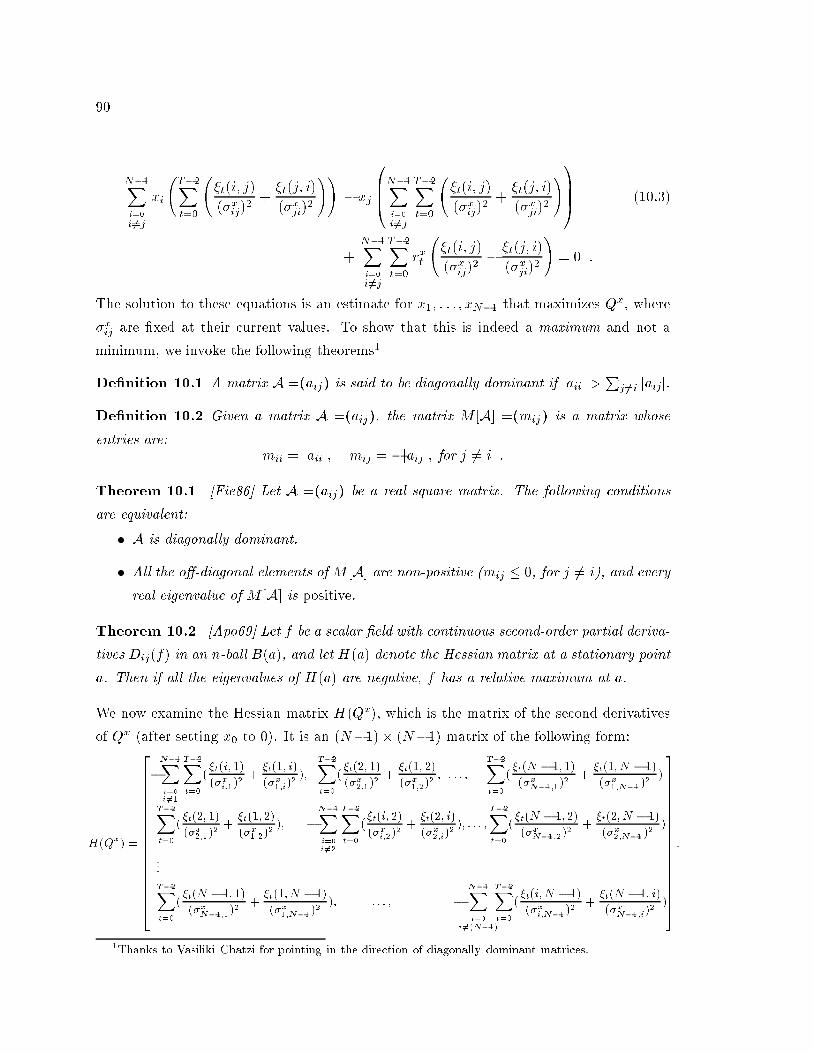
90 N�1Xi=0i 6=j xi T�2Xt=0 �t(i; j)(�xij)2 + �t(j; i)(�xji)2 !! � xj 0BB�N�1Xi=0i 6=j T�2Xt=0 �t(i; j)(�xij)2 + �t(j; i)(�xji)2 !1CCA (10.3)+ N�1Xi=0i 6=j T�2Xt=0 rxt �t(i; j)(�xij)2 � �t(j; i)(�xji)2 ! = 0 :The solution to these equations is an estimate for x1; : : : ; xN�1 that maximizes Qx, where�xij are �xed at their urrent values. To show that this is indeed a maximum and not aminimum, we invoke the following theorems1De�nition 10.1 A matrix A =(aij) is said to be diagonally dominant if jaiij >Pj 6=i jaijj.De�nition 10.2 Given a matrix A =(aij), the matrix M [A℄ =(mij) is a matrix whoseentries are: mii = jaiij; mij = �jaij j; for j 6= i :Theorem 10.1 [Fie86℄ Let A =(aij) be a real square matrix. The following onditionsare equivalent:� A is diagonally dominant.� All the o�-diagonal elements of M [A℄ are non-positive (mij � 0, for j 6= i), and everyreal eigenvalue of M [A℄ is positive.Theorem 10.2 [Apo69℄ Let f be a s alar �eld with ontinuous se ond-order partial deriva-tives Dij(f) in an n-ball B(a), and let H(a) denote the Hessian matrix at a stationary pointa. Then if all the eigenvalues of H(a) are negative, f has a relative maximum at a.We now examine the Hessian matrix H(Qx), whi h is the matrix of the se ond derivativesof Qx (after setting x0 to 0). It is an (N�1)� (N�1) matrix of the following form:H(Qx) = 266666666666666664�N�1Xi=0i6=1 T�2Xt=0 (�t(i; 1)(�xi;1)2 + �t(1; i)(�x1;i)2 ); T�2Xt=0 (�t(2; 1)(�x2;1)2 + �t(1; 2)(�x1;2)2 ; : : : ; T�2Xt=0 (�t(N � 1; 1)(�xN�1;1)2 + �t(1;N � 1)(�x1;N�1)2 )T�2Xt=0 (�t(2; 1)(�x2;1)2 + �t(1; 2)(�x1;2)2 ); �N�1Xi=0i6=2 T�2Xt=0 (�t(i; 2)(�xi;2)2 + �t(2; i)(�x2;i)2 ); : : : ; T�2Xt=0 (�t(N � 1; 2)(�xN�1;2)2 + �t(2;N � 1)(�x2;N�1)2 ):::T�2Xt=0 (�t(N � 1; 1)(�xN�1;1)2 + �t(1;N � 1)(�x1;N�1)2 ); : : : ; � N�1Xi=0i6=(N�1)T�2Xt=0 (�t(i;N � 1)(�xi;N�1)2 + �t(N � 1; i)(�xN�1;i)2 )377777777777777775 :1Thanks to Vasiliki Chatzi for pointing in the dire tion of diagonally dominant matri es.

91Under the assumption that all �t's are stri tly positive, we note that H(Qx) is diagonallydominant, sin e all its diagonal elements are stri tly larger in magnitude than the sum ofthe other elements in their respe tive rows. Hen e, by theorem 10.1 all the eigenvalues ofthe matrix M [H(Qx)℄ are positive. Note that M [H(Qx)℄ = �H(Qx), and that from thede�nition of eigenvalues, k is an eigenvalue of �H(Qx) if and only if �k is an eigenvalue ofH(Qx). Therefore all the eigenvalues of the Hessian H(Qx) itself are negative and thereforeby theorem 10.2, Qx is indeed maximized when the lo ations for the states are hosen assolutions to the above equations.An estimate for ea h mean relation �xij is simply obtained as�xij = xj � xi ; (10.4)and all the geometri al onstraints are met. The pro edure for y is identi al. The pro essfor reestimating the varian e remains as des ribed in Se tion 4.2.2.10.2 Additivity within a Relative FrameworkIn Se tion 8.2 we expressed the geometri al onsisten y onstraints in the ontext of relative oordinate systems. In this s enario, ea h state has asso iated with it a oordinate systemwhose origin is at the state, its y axis is aligned with the heading asso iated with the state,and its x axis is perpendi ular to it (see, for instan e, Figure 8.3).To enfor e the geometri al onsisten y onstraints dire tly, we observe again that it issuÆ ient to asso iate points hx0; y0; �0i; : : : ; hxN�1; yN�1; �N�1i with the states s0; : : : ; sN�1,respe tively, only that this time the relationships between states along the x and y dimen-sions are interdependent through the hange in headings between the states.We denote by (�xij)0 = x0j � x0i and (�yij)0 = y0j � y0i the mean odometri relation fromstate si to state sj with respe t to the global oordinate system whose origin is at state s0,along the global x and y axes, respe tively. If state si has mean heading ��0;i with respe tto the heading at state s0, then with respe t to state si,(�xij)i = os(��0;i)(�xij)0 � sin(��0;i)(�yij)0 = os(��0;i)(x0j � x0i )� sin(��0;i)(y0j � y0i ) :Similarly,(�yij)i = sin(��0;i)(x0j � x0i ) + os(��0;i)(y0j � y0i ) :

92We note that the re orded relations rxt ; ryt are also expressed with respe t to the heading attime t. Thus, we are left with the following expression for maximization:Qx;y(R;R) = N�1Xi=0 N�1Xj=0 T�2Xt=0 �t(i; j) �(rxt+1 � �xij)22(�xij)2 � log(�xij) � (ryt+1 � �yij)22(�yij)2 � log(�yij)!= N�1Xi=0 N�1Xj=0 T�2Xt=0 �t(i; j) �(rxt+1 � ( os(��0;i)(x0j � x0i )� sin(��0;i)(y0j � y0i )))22(�xij)2� log(�xij) � (ryt+1 � (sin(��0;i)(x0j � x0i ) + os(��0;i)(y0j � y0i )))22(�yij)2 � log(�yij)! : (10.5)Di�erentiating equation 10.5 a ording to ea h x0j and ea h y0j where j 6= 0 , and equatingea h partial derivative to 0, results in a set of 2N�2 linear equations in 2N�2 unknowns.(The derivatives and the equations are given in Appendix B.2.) The solution, obtained aspart of ea h em iteration, is a set of oordinates x1; : : : ; xN�1, y1; : : : ; yN�1; for the statess1; : : : ; sN�1 , respe tively. As before, s0 is set to be at h0; 0i.The mean state relationships, �xij ; �yij are re overed through the equations:(�xij)i = os(��0;i)(x0j � x0i )� sin(��0;i)(y0j � y0i ) ; (10.6)(�yij)i = sin(��0;i)(x0j � x0i ) + os(��0;i)(y0j � y0i ) : (10.7)Note that the underlying assumption used here is that an estimate for the mean angle ��0;iis already al ulated. Obtaining geometri ally onsistent heading angles is dis ussed in thefollowing se tion.10.3 Additive Heading EstimationThe method demonstrated so far suggested that �nding optimal state oordinates and de-du ing the relationships between them rather than dire tly �nding optimal relationships isa good way to address the additivity onstraint. Unfortunately, this approa h is hard to fol-low in the ase of heading hange estimation, due to the von Mises distribution assumptionof the heading measures.Re all that the von Mises density fun tion has the form:f�;�(�) = 12�I0(�)e� os(���) ;where I0(�) is the modi�ed Bessel fun tion of the �rst kind and order 0, I0(�) = 1Xr=0 1r!2 (12�)2r:Hen e, by substituting �ij by �j � �i and applying a pro edure similar to the one dis ussed

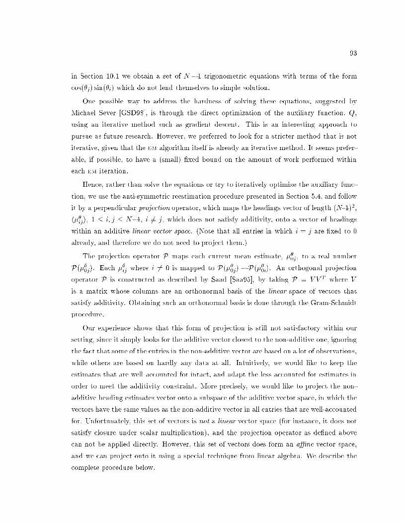
93in Se tion 10.1 we obtain a set of N�1 trigonometri equations with terms of the form os(�j) sin(�i) whi h do not lend themselves to simple solution.One possible way to address the hardness of solving these equations, suggested byMi hael Sever [GSD98℄, is through the dire t optimization of the auxiliary fun tion, Q,using an iterative method su h as gradient des ent. This is an interesting approa h topursue as future resear h. However, we preferred to look for a stri ter method that is notiterative, given that the em algorithm itself is already an iterative method. It seems prefer-able, if possible, to have a (small) �xed bound on the amount of work performed withinea h em iteration.Hen e, rather than solve the equations or try to iteratively optimize the auxiliary fun -tion, we use the anti-symmetri reestimation pro edure presented in Se tion 5.4, and followit by a perpendi ular proje tion operator, whi h maps the headings ve tor of length (N�1)2,h��iji; 1 � i; j � N�1, i 6= j, whi h does not satisfy additivity, onto a ve tor of headingswithin an additive linear ve tor spa e. (Note that all entries in whi h i = j are �xed to 0already, and therefore we do not need to proje t them.)The proje tion operator P maps ea h urrent mean estimate, ��0j , to a real numberP(��0j). Ea h ��ij where i 6= 0 is mapped to P(��0j) � P(��0i). An orthogonal proje tionoperator P is onstru ted as des ribed by Saad [Saa95℄, by taking P = V V T where Vis a matrix whose olumns are an orthonormal basis of the linear spa e of ve tors thatsatisfy additivity. Obtaining su h an orthonormal basis is done through the Gram-S hmidtpro edure.Our experien e shows that this form of proje tion is still not satisfa tory within oursetting, sin e it simply looks for the additive ve tor losest to the non-additive one, ignoringthe fa t that some of the entries in the non-additive ve tor are based on a lot of observations,while others are based on hardly any data at all. Intuitively, we would like to keep theestimates that are well a ounted for inta t, and adapt the less a ounted for estimates inorder to meet the additivity onstraint. More pre isely, we would like to proje t the non-additive heading estimates ve tor onto a subspa e of the additive ve tor spa e, in whi h theve tors have the same values as the non-additive ve tor in all entries that are well-a ountedfor. Unfortunately, this set of ve tors is not a linear ve tor spa e (for instan e, it does notsatisfy losure under s alar multipli ation), and the proje tion operator as de�ned above an not be applied dire tly. However, this set of ve tors does form an aÆne ve tor spa e,and we an proje t onto it using a spe ial te hnique from linear algebra. We des ribe the omplete pro edure below.

9410.3.1 Sele ting Fixed EntriesWe start by pi king the maximum number, n, of heading estimates that we would like topreserve. A typi al hoi e we have made is for n to be the number of states in the model.Using the heap data stru ture over all expe ted ounts of transitions between states, wesele t a list of the n ordered pairs of states (si; sj) that have the largest expe ted transition ounts, Pt(�ij), from si to sj . The list is kept sorted a ording to the number of theexpe ted ounts. Note that we an't just �x these values and pro eed to the proje tionstage, sin e:1. There may be in onsisten ies between these topmost values themselves;2. By �xing ertain relationships, other relationships are also enfor ed through the geo-metri al onsisten y requirement.Therefore �xing the entries that should not be proje ted requires examining and propagatingdependen ies within the heading relationship ve tor. To allow for easy expression of theinterdependen ies, we hoose to take ��0;1; : : : ; ��0;N�1 as independent variables, and expressthe rest of the relationships ��i;j as ��0;j � ��0;i.Building the �xed-values ve tor pro eeds as follows. We pi k the most a ounted forrelationship ��i1;j1 , and assume its estimated value is �1. Fixing it implies that the ve torentry for ��j1;i1 is set to ��1. Note that on e the entry is �xed it does not hange any more.That is, if later in the list of sorted state pairs there is a ontradi ting assignment to ��j1;i1 ,we dis ard this item in the sorted list without using it to �x any of the values, and movedown to the next item in the list. However, we do not add any more items to the list; thuswe may, in pra ti e, use less than the n most a ounted for values.We also note that �xing ��j1;i1 impli itly for es the relationship between ��0;i1 and ��0;j1to be ��0;i1 = ��0;j1 + �1.On e all the impli it relationships are determined, the next most a ounted for item onthe list is examined. As said before, if it is in onsistent with the already �xed values, itis dis arded. Else, it is used for �xing all the impli it dependents. We pro eed until all nitems in the sorted list are treated.At the end of this phase we have entries that are ompletely determined, with a numeri alvalue assigned to them, as well as entries that are inter-related su h as ��0;i1 above whi hdepends on ��0;j1 through the equation: ��0;i1 = ��0;j1 + �1. Sin e, obviously, ��0;i1 and��0;j1 depend on one another, we adopt the onvention that the item with the higher index

95depends on the the item with the lower index, and the item with the lower index is viewedas a free variable. The following example demonstrates the pro ess.Example 10.1 Suppose our model has 3 states. Hen e our estimated symmetri ve tor ofheading relationships, ex luding self-transitions values whi h are always 0, has 6 entries.h��0;1; ��0;2; ��1;0; ��1;2; ��2;0; ��2;1i = h90; 110;�90; 5;�110;�5i :We note that ��0;1 + ��1;2 is urrently not equal to ��0;2. Now, suppose that our expe tedsupporting ounts of transitions between every pair of states are as follows:0 1 20 0.01 0.01 0.011 0.02 0.01 3.972 0.01 2.94 0.03Suppose we are only going to preserve the relationships for the 2 most a ounted for statetransitions. Hen e our sorted list ontains is ��1;2; ��2;1. By �xing ��1;2 to 5 we �x ��2;1 to�5, and ��0;2 = ��0;1 + 5. (Through symmetry we have ��1;0 = ���0;1 and ��2;0 = ���0;1 � 5.)The se ond most-supported value is ��2;1, but sin e it was already �xed by the previous step| we are done. The geometri ally onsistent partially-�xed ve tor is now:h��0;1; ��0;1 + 5; ���0;1; 5; ���0;1 � 5; �5i :The �nal step left is to proje t the in onsistent values urrently assigned to the un�xedentries h90; 110;�90;�110i onto a spa e of the form hx; x+5;�x;�x�5i.We emphasize again, that ve tors of the form hx; x+5;�x;�x�5i do not onstitutea linear ve tor spa e. In ontrast, ve tors of the form hx; x;�x;�xi do onstitute a lin-ear spa e. An aÆne transformation maps between these two spa es; adding/subtra tingthe ve tor h0; 5;�0;�5i is the appropriate transformation. Hen e, ve tors of the formhx; x+5;�x;�x�5i onstitute an aÆne spa e of ve tors. The following se tion explainshow to proje t onto su h a spa e.10.3.2 Proje tion onto an AÆne Spa e 2Perpendi ular proje tion onto a linear spa e was des ribed earlier in this hapter. An aÆnespa e A is de�ned as follows:2This se tion is almost ompletely based on material I learned through onversations with John Hughes,to whom I am most grateful.

96-2 2 4

-4

-2

2

4

6

v

Ta(v)

P(v)

P(Ta(v))

<x,-x>

<x,-x+4>

Figure 10.1: Proje ting v onto an aÆne spa eDe�nition 10.3 A � Rn is an n-dimensional aÆne spa e if for all ve tors va 2 A, the setof ve tors: A� va def= fua � vajua 2 Ag is a linear spa e.Hen e, we an pi k a ve tor va1 2 A and de�ne the translation Ta : A ! V , where V is alinear spa e, V = A � va1 . This translation is trivially extended for any ve tor v0 2 Rn,by de�ning Ta(v0) = v0 � va1 . In order to proje t a ve tor v 2 Rn onto A, we apply thetranslation Ta to v and proje t Ta(v) onto V , whi h results in a ve tor P(Ta(v)) in V . Byapplying the inverse transform T�1a to it, we obtain the proje tion of v on A.This pro ess is demonstrated in Figure 10.1, in whi h the linear spa e is the two di-mensional ve tor spa e fhx; yij y = �xg, and the aÆne spa e is fhx; yij y = �x + 4g. Thetransform Ta in this ase onsists of subtra ting the ve tor h0; 4i. The solid arrow in the�gure orresponds to the dire t proje tion of the ve tor v onto the point P(v) of the aÆnespa e. The dashed arrows represent the proje tion via translation of v to Ta(v), the pro-je tion of the latter onto the linear ve tor spa e, and the inverse translation of the result,P(Ta(v)), onto the aÆne spa e.By applying this proje tion pro ess, we obtain the values that repla e the entries in theheading relations ve tor that were not yet �xed by the previous stage of the algorithm, anddid not satisfy additivity. We plug these values into their orre t entries in the ve tor andobtain a heading ve tor that satis�es additivity. We note that it is suÆ ient to proje tonly the entries orresponding to unde�ned values of �0;1; : : : ; �0;N�1; the rest of the values an be dedu ed through the expression: �i;j = �0;j � �0;i. We on lude this se tion by ompleting the example provided earlier.

97Example 10.1 (Cont.) We needed to proje t the values h90; 110;�90;�110i onto a spa eof the form hx; x+ 5;�x;�x� 5i. It is suÆ ient to proje t the entries h90; 110i onto thespa e hx; x+ 5i, and the rest of the values are obtained through anti-symmetry. The linearspa e hx; xi is obtained from the aÆne spa e hx; x+ 5i through the transform of subtra tingthe ve tor h0; 5i. Applying this transform to the ve tor h90; 110i results in h85; 105i. Thespa e hx; xi is spanned by the orthonormal basis b = h 1p2 ; 1p2i. The proje tion obtained bytaking bTb applied to the ve tor h85; 105i results in the ve tor h95; 95i. We apply the inversetranslation, adding h0; 5i and obtain the ve tor h95; 100i.The omplete ve tor obtained by plugging h95; 100;�95;�100i into the yet undeterminedentries of the heading relations ve tor gives us the following additive heading reestimate:h95; 100;�95; 5;�100;�5i :Although the pro edure for preserving additivity over headings is not proven to preservemonotone onvergen e of the likelihood fun tion towards a lo al maximum, our experimentshave shown that monotone onvergen e is preserved. However, under the urrent form ofadditivity enfor ement, the quality of the results, as demonstrated in the next hapter, ompared with those obtained when only symmetry is enfor ed, does not learly justify theadditional e�ort involved.

98

Chapter 11Experiments Enfor ing AdditivitySimilar to the experiments presented in previous hapters, we test the algorithm both withina global framework under the perpendi ularity assumption, and within a relative oordinateframework, where the perpendi ularity assumption is relaxed. Again, we use both real robotdata and data obtained from the same simulated model as before.As before, we provide both qualitative results in terms of plots of the models, and statis-ti al evaluation. Se tion 11.1 demonstrates the e�e ts of additivity enfor ement under theperpendi ularity assumption, while Se tion 11.2 demonstrates its e�e ts when the perpen-di ularity assumption is relaxed. Note that there is a signi� ant di�eren e between the twosettings. The reason is that when the perpendi ularity assumption is dropped, obtainingthe orre t headings is ru ial, sin e the evaluation of both x and y measurements dependon the heading. Through the use of proje tion over the heading we ompromise the qualityof the heading, and possibly harm x and y estimates. Another problem with the additivityenfor ement is its relian e on �0i as a basis for the onstraints. A bad estimate for the �0i's an result in a bad estimation of all the geometri al parameters.Se tion 11.3 des ribes some experiments designed spe i� ally for studying the e�e ts ofodometry and additivity on the quality of the topology and the geometry of learnt models.11.1 Results within a Global FrameworkWe applied the algorithm des ribed in Se tion 10.1 to the same robot-gathered and simu-lated sequen es des ribed and used in Chapter 7. The same evaluation methods are appliedhere as well. 99

1000

15

16

1

2

3 4 5 6 7 8

9

10

11

12

1314

3 5 6 7 84

9

10

11

12

1314150

16

1

2

6

2

1316 0 5

15

349

7

1

8

10

11

12

14

Figure 11.1:Learned model of the orridorsRamona traversed. Initialization is Tag-based. Figure 11.2:Learned model of the orridorsRamona traversed. Initialization is k-meansbased.15

6

3

13 14 12

2

8

17

4

16

95

10

11

0

13 14 12

2

0

16

74

510

11

1 9

8

6

15

3

11

0

71

5

2

10

14 15

13

412

3

6

8

16

9

1

5

8

2

10

14 15 913

412

3

11

0716 6Figure 11.3:Learned model of the orridorsRamona traversed. Initialization is k-meansbased. Figure 11.4:Learned model of the orridorsRamona traversed. Initialization is random.Figures 11.1 { 11.4 show some of the models obtained by applying our algorithm en-for ing the omplete geometri al onsisten y while using the various initialization methods.Bold dashed arrows denote transitions whose probability is very lose to the probability ofthe most likely transition from the state. The most a urate map is learned using the tag-based initialization te hnique. There is very little u tuation in the quality of the modelsa ross multiple runs sin e the initialization is lose to deterministi (up to the random noisesuperimposed on the data). However, this model is not very di�erent from the one depi ted

101in Figure 7.3 whi h was learned without enfor ing additivity, using the same initializationalgorithm.The two examples of the learned geometry starting from k-means initialization demon-strate that geometri ally onsistent models an still vary in quality. Moreover, althoughthe geometry looks almost a urate in Figure 11.2, note that the topology is still not asgood, given that we don't have two states at ea h of the top two orners to denote hangeof headings during turns, and that there is a ba k and forth transition between states13 and 16. The variability in the geometri al outline of the models a ross multiple runs,when starting with k-means initialization is smaller when additivity is enfor ed, than whenonly anti-symmetry is enfor ed. That is, we get more onsistently good models and thedependen e on the initial lustering seems to be redu ed.It is interesting to note that even when starting from a random initial model, the algo-rithm did onverge several times to models with geometry that is lose to the true one, asshown in Figure 11.4. Again, this behavior appears to o ur more onsistently than whenonly anti-symmetry is enfor ed.Figures 11.5 { 11.8 show some of the models obtained by applying our algorithm to thesimulated sequen es, enfor ing the omplete geometri al onsisten y while using the variousinitialization methods. The most a urate map, shown in Figure 11.5 is learned using thek-means based initialization te hnique. Using a global framework allows this method tobe e�e tive. There is still, however, a lot of variability a ross multiple runs and trainingsequen es, in the quality of the results under this initialization method, due to its randomstarting point. A mu h worse model, geometri ally speaking, whi h does not represent thetrue environment well, despite its geometri al onsisten y, is shown in Figure 11.6. Whenusing the tag-based initialization, we get more uniformity in the quality of the results a rossmultiple runs, but there is still diversity when running over di�erent data sequen es. Weshow one of the better geometri al models in Figure 11.7, and not as good a model inFigure 11.8. A possible explanation to the diversity in quality of the learned simulatedmodel, under tag-based initialization, as opposed to the models learned from robot data,is that the simulated environment is mu h larger. This auses the global relations betweenremote states, whi h are re e ted in the geometri al onsisten y onstraints, to be harderto learn.For the purpose of quantitatively evaluating the learning algorithm we provide in Ta-ble 11.1 a summary of the results of running the algorithm under ea h of the 3 initializationsettings, 10 times for ea h sequen e. The results of the runs without odometri information

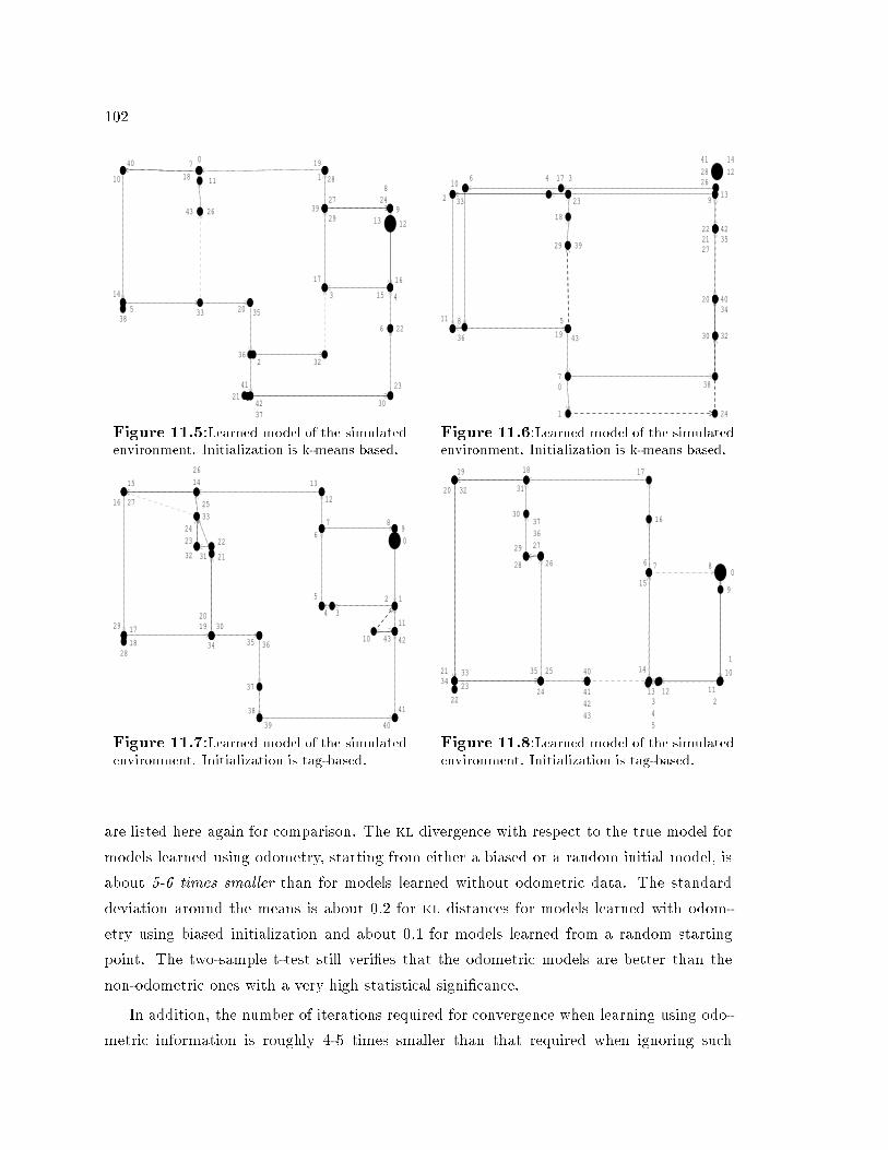
10212

153

17

39

28

19040

10

14

5 33 20 35

36

41

42 30

23

22

4

6

2 32

27 249

13

16

38

26

1118

43

37

7

29

81

21

14

12

422221

4034

20

27

13

26410

2

11

36 19

5

43

70 38

39

18

23

3

29

1 24

32

35

30

41

28

9

176

33

8Figure 11.5:Learned model of the simulatedenvironment. Initialization is k-means based. Figure 11.6:Learned model of the simulatedenvironment. Initialization is k-means based.0

12

34

5

6

12

131415

16 27

18

29

34 35 36

37

38

39 40

41

424310

11

7 89

26

30

22

3132

23

3324

25

28

21

17 1920

0

9

10

111213

14

15

76

16

171819

20

21

2324

40

4142

25

26

27

28

29

30

31

8

32

3334

1

43

22

35

2345

3637

Figure 11.7:Learned model of the simulatedenvironment. Initialization is tag-based. Figure 11.8:Learned model of the simulatedenvironment. Initialization is tag-based.are listed here again for omparison. The kl divergen e with respe t to the true model formodels learned using odometry, starting from either a biased or a random initial model, isabout 5-6 times smaller than for models learned without odometri data. The standarddeviation around the means is about 0.2 for kl distan es for models learned with odom-etry using biased initialization and about 0.1 for models learned from a random startingpoint. The two-sample t-test still veri�es that the odometri models are better than thenon-odometri ones with a very high statisti al signi� an e.In addition, the number of iterations required for onvergen e when learning using odo-metri information is roughly 4-5 times smaller than that required when ignoring su h

103Seq. Tag-based k-means Random No Odo# kl Iter.# kl Iter. # kl Iter. # kl Iter. #1 0.981 16.70 1.149 29.90 1.061 28.40 6.351 124.12 1.290 20.90 1.037 27.80 1.037 27.70 4.863 126.03 1.115 22.30 1.085 20.40 1.110 21.50 5.926 113.04 1.241 12.70 1.144 26.60 1.055 19.90 6.261 107.45 1.241 27.50 1.442 20.40 1.028 29.20 4.802 122.9Table 11.1: Average results of four learning settings with �ve training sequen es.information. Again, the t-test veri�es the signi� an e of this result. As before, the num-ber of iterations required for onvergen e when starting from a tag-based initial model isstatisti ally signi� antly lower than when starting with any other initialization method.Under all three initialization settings, the models learned are topologi ally somewhatinferior (and this is with high statisti al signi� an e), in terms of the kl divergen e, tothose learned without enfor ing additivity. This is likely to be a result of the very strong onstraints enfor ed during the learning pro ess, whi h prevent the algorithm from sear hingbetter areas of the learning-spa e, and restri t it to rea h poor lo al maxima. The geometrylooks superior in some ases, but it is not signi� antly better. However, there seems to beless variability in the quality of the geometri al models a ross multiple runs when additivityis enfor ed.11.2 Results within a Relative FrameworkWe applied the algorithm des ribed in Se tion 10.2 to the same robot-gathered and sim-ulated sequen es des ribed and used in Chapter 9. The evaluation methods also stay thesame. Figure 11.9 shows a typi al model obtained by applying the algorithm enfor ing the omplete geometri al onsisten y, to the robot data shown in Figure 9.3, using tag-basedinitialization. The enfor ement of onsisten y onstraints resulted in a better preservationof the re tangular geometry of the environment. We noti e that state 0 still does not par-ti ipate in the loop. The main reason for this is that due to the relatively large number ofstates that are lose together in the orresponding area of the true environment, it was notre ognized that we ever returned to this parti ular state during the loop. Therefore, therewas only one transition re orded from state 0 to state 1 a ording to the expe ted transition ounts al ulated by the algorithm. When proje ting the angles to maintain additivity, theangle from state 0 to 1 was therefore ompromised, allowing geometri al onsisten y to

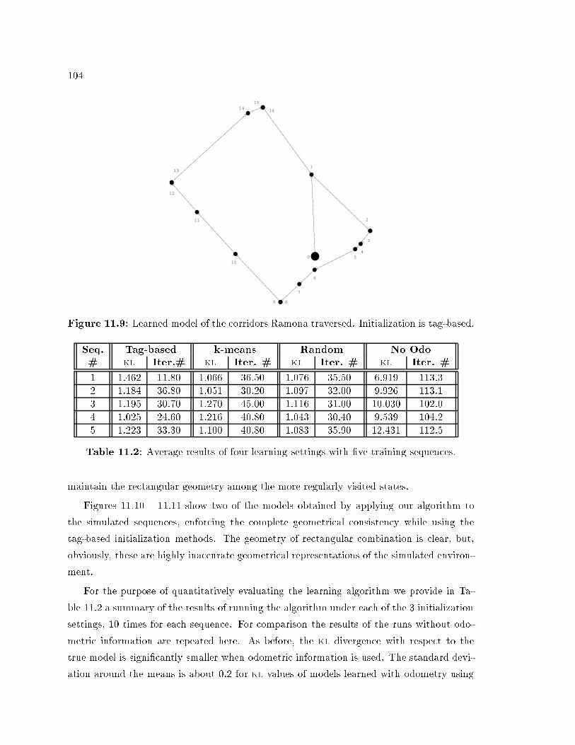
1040

1

2

3

45

6

7

89

10

11

12

13

1415

16

Figure 11.9: Learned model of the orridors Ramona traversed. Initialization is tag-based.Seq. Tag-based k-means Random No Odo# kl Iter.# kl Iter. # kl Iter. # kl Iter. #1 1.462 11.80 1.066 36.50 1.076 35.50 6.919 113.32 1.184 36.80 1.051 30.20 1.097 32.00 9.926 113.13 1.195 30.70 1.270 45.00 1.116 31.00 10.030 102.04 1.025 24.60 1.216 40.80 1.043 30.40 9.539 104.25 1.223 33.30 1.100 40.80 1.083 35.90 12.431 112.5Table 11.2: Average results of four learning settings with �ve training sequen es.maintain the re tangular geometry among the more regularly visited states.Figures 11.10 { 11.11 show two of the models obtained by applying our algorithm tothe simulated sequen es, enfor ing the omplete geometri al onsisten y while using thetag-based initialization methods. The geometry of re tangular ombination is lear, but,obviously, these are highly ina urate geometri al representations of the simulated environ-ment.For the purpose of quantitatively evaluating the learning algorithm we provide in Ta-ble 11.2 a summary of the results of running the algorithm under ea h of the 3 initializationsettings, 10 times for ea h sequen e. For omparison the results of the runs without odo-metri information are repeated here. As before, the kl divergen e with respe t to thetrue model is signi� antly smaller when odometri information is used. The standard devi-ation around the means is about 0.2 for kl values of models learned with odometry using

105Figure 11.10:Learned model of the simu-lated environment. Figure 11.11:Learned model of the simu-lated environment.tag-based initialization and about 0.1 for models learned from a random or k-means-basedstarting point.The standard deviation around the number of iterations is about 10 for models startedfrom either a random or a tag-based model and about 20 for models whose initializationwas based on k-means. The number of iterations when additivity is enfor ed in the relative oordinate setting is onsistently higher, with high statisti al signi� an e, than when onlyanti-symmetry is enfor ed, in the ase of k-means based initialization. An explanation forthis is that in the relative setting, the bad initialization starting from k-means leads to lowlikelihood values, whi h in turn auses numeri al instability in the pro ess of solving the setof equations required for enfor ing additivity. This auses a slowdown in the onvergen eof the em algorithm. An in rease in the number of iterations, whi h is not as dramati and not as statisti ally signi� ant, also exists when using any of the other two initializationmethods.11.3 Studying the E�e ts of Odometry and AdditivityTo better understand the impa t of enfor ing geometri al onsisten y in parti ular andthat of odometri information in general, we study two small examples. We designed twomodels; One that intuitively does not require additivity in order to be learned, and the otherwhi h seemingly does require the enfor ement of the omplete geometri al onsisten y. Wesampled data from both models, and applied our algorithms to it. The models, and theresults analysis are des ribed throughout the rest of this se tion.

106 0< D, W, W> 1< O, D, D> 2< O, D, D> 3< O, D, D> 4< O, D, D>0.85 0.85 0.85 0.850.85 0< D, W, W> 1< O, D, D> 2< O, D, D> 3< O, D, D> 4< O, D, D>0.22 0.78 0.94 0.81 0.85

0.82Figure 11.12:A model of a simulated en-vironment. The distan es between states aredrawn to s ale. Initial state is distin t. Figure 11.13:A learned model. Initializa-tion is Tag-based. Distan es are drawn tos ale.2< D, W, W> 4< O, D, D> 3< O, D, D> 0< O, D, D> 1< O, D, D>0.850.82

0.22 0.78 0.810.94 4< O, D, D> 3< O, D, D> 2< O, D, D> 1< O, D, D>0< D, W, W>0.22 0.780.81

0.850.810.94Figure 11.14:A learned model. Initializa-tion is k-means based. Figure 11.15:A learned model. Initializa-tion is k-means based.Experiment 11.1 To examine the e�e ts of odometri information on learning a model,we used a small y li model, for whi h the initial state has a distin t tuple of observations,while all other states look alike observation-wise, but an be distinguished by their geomet-ri al pla ement in the environment. Figure 11.12 shows a geometri layout of the modelas a probabilisti state-transition diagram. Note that the states are pla ed in di�erent dis-tan es from ea h other. This pla ement is signi� ant, and represents the geometry of thestate spa e; all the states lie on the same line, with diminishing distan es from one state tothe next. The distan es between the states in the �gure are drawn to s ale. Edges denotetransitions with probability greater than 0:2. The numbers on the edges orrespond to thea tual transition probabilities. At ea h state, the observations onsist of the view on thefront, left and right, whi h an be either a door, D, a wall, W, or and open area O. Themost likely observations are shown in the diagram. These observations are typi ally seen80-90 per ent of the times when a state is visited.Using Monte-Carlo sampling we generated two sequen es of 300 observations and learned5 models from ea h of them under ea h of the four learning settings, enfor ing only anti-symmetry during the learning pro ess.Figure 11.13 shows a typi al model learned using tag-based initialization. Again, thestates are pla ed a ording to the relation matrix learned. It is lear that there is an almostperfe t orresponden e between both the geometry and the topology under this learningsetting. All models learned using this algorithm look almost identi al to this one.

1073< O, D, D> 2< O, D, D> 0< O, D, D> 1< O, D, D>4< D, W, W> 0.850.81

0.790.940.780.224< O, D, D> 0< O, D, D>1< O, D, D>2< D, W, W>3< D, W, W>

0.40 0.420.910.500.500.790.21 0.85Figure 11.16:A learned model. Initializa-tion is random. Figure 11.17:A learned model. Initializa-tion is random.3< D, W, W> 4< O, D, D> 2< O, D, D> 0< O, D, D> 1< D, W, W>0.37 0.21

0.42 0.51 0.490.570.430.88 0.730.27 3< O, D, D> 0< D, W, W> 4< O, D, D> 1< D, O, W> 2< D, W, W>0.87 0.440.560.81

0.280.63 0.46 0.54Figure 11.18:A learned model. No odome-try used. State pla ing is arbitrary, Figure 11.19:A learned model. No odome-try used. State pla ing is arbitrary.Figures 11.14 and 11.15 demonstrate the results of learning using k-means based ini-tialization. The �gure on the left shows a typi al good result, where both topology andgeometry almost exa tly �t the true model. However, when starting from a poor lustering,the model is not as good; although it is still topologi ally orre t, the initial state is not orre tly identi�ed. This is shown in Figure 11.15.Figures 11.16 and 11.17 show the results of learning starting from a randomly initializedmodel. The �gure on the left shows the less frequent ase in whi h the algorithm managed tolearn a good model despite the random initialization. The �gure on the right demonstratesone of the less well-learned models, in whi h the geometry is learly not as good as inall the other odometri model. The two leftmost states are a tually pla ed in the sameposition a ording to the relation matrix, and are pla ed one above the other for the sakeof readability only. These two states orrespond the initial state in the original model. The y li ity is still present and the observations are still the same as in the original model, butboth the topologi al and the geometri al stru ture is di�erent from the true one.Figures 11.18 and 11.19 show the results of learning without the use of odometry. Itis important to note that the pla ement of the states here has no geometri al signi� an e,and the layout is imposed in order to larify the plot. Figure 11.18 depi ts one of thebetter models, in whi h the observation distribution orresponds well to that of the originalmodel although the topology is di�erent. In Figure 11.19, we see that in state 1, the triplehD; O; W i that is highly unlikely in the original model was learned as a likely observationtriple, although, in an unlikely-to-be-rea hed state.

108 Seq. Tag-based k-means Random No Odo# Mean StD Mean StD Mean StD Mean StD1 0.073 0.019 0.641 0.766 0.699 0.101 0.609 0.1982 0.032 0.006 0.091 0.067 0.805 0.239 0.987 1.117Table 11.3: Average results of four learning settings with two training sequen es.We an see that under this setting, odometry greatly helps to distinguish the states fromea h other, and the tag-based initialization ensures onsistently good results.To verify these results we also used the Kullba k-Liebler divergen e, evaluated based ongenerating 50 sequen es of length 20 ea h from the true model and measuring the di�eren ebetween their likelihood with respe t to the true model and the likelihood with respe tto the learned model (averaging over the total number of data points { 1000 in this ase).Table 11.3 lists the means and standard deviations of the Kullba k-Leibler measure for ea hof the sequen es averaged over the 5 di�erent learning experien es. The kl divergen e formodels learned using tag-based initialization are mu h smaller than for those learned usingany other initialization method, or not using odometry at all. Using k-means based initial-ization typi ally gives very good results in this setting, but due to two severe outliers whenstarting from bad initial lustering, the mean is not mu h lower than when using randominitialization or no odometry in the ase of the �rst sequen e. Note that the geometri alsetting of the model is su h that there are no turns, and therefore umulative rotationalerror does not interfere with the e�e tiveness of the k-means based initialization. (Still,the algorithm used here does take into a ount umulative rotational errors, as des ribedin Chapter 9.)Models learned using odometry, starting from a random initialization, are not mu hbetter than those learned without odometri information at all, although, at times theformer still does very well, while the latter sometimes performs mu h worse. (Spe i� ally,when using the se ond sequen e the di�eren e between the two settings is apparent). Itis important to note that the example uses a small model whi h is not very peaked, andthat there was an abundan e of data provided from it. Hen e, even the non-odometri learning performed quite well, if all we are on erned about is the probability distributionover sequen es.Experiment 11.2 To examine the e�e ts of enfor ing additivity on the learning pro ess,it takes a model in whi h not only is odometry needed to distinguish between seeminglysimilar states, but also, odometry helps to tell that a state rea hed via two distin t routes

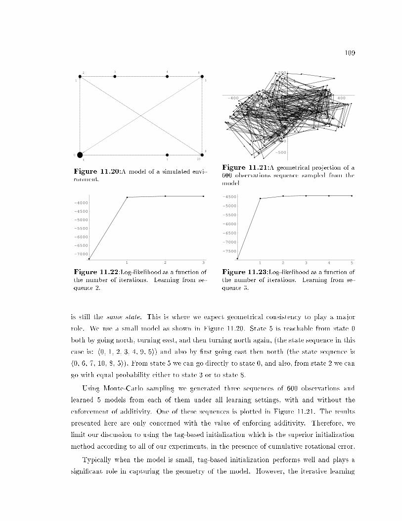
1090

1

2 3 4 9

5

6 7 10

8

-400 -200 200 400

-500

-400

-300

-200

-100

100

200

Figure 11.20:A model of a simulated envi-ronment. Figure 11.21:A geometri al proje tion of a600 observations sequen e sampled from themodel1 2 3

-7000

-6500

-6000

-5500

-5000

-4500

-4000

1 2 3 4 5

-7500

-7000

-6500

-6000

-5500

-5000

-4500Figure 11.22:Log-likelihood as a fun tion ofthe number of iterations. Learning from se-quen e 2. Figure 11.23:Log-likelihood as a fun tion ofthe number of iterations. Learning from se-quen e 3.is still the same state. This is where we expe t geometri al onsisten y to play a majorrole. We use a small model as shown in Figure 11.20. State 5 is rea hable from state 0both by going north, turning east, and then turning north again, (the state sequen e in this ase is: h0; 1; 2; 3; 4; 9; 5i) and also by �rst going east then north (the state sequen e ish0; 6; 7; 10; 8; 5i). From state 5 we an go dire tly to state 0, and also, from state 2 we ango with equal probability either to state 3 or to state 8.Using Monte-Carlo sampling we generated three sequen es of 600 observations andlearned 5 models from ea h of them under all learning settings, with and without theenfor ement of additivity. One of these sequen es is plotted in Figure 11.21. The resultspresented here are only on erned with the value of enfor ing additivity. Therefore, welimit our dis ussion to using the tag-based initialization whi h is the superior initializationmethod a ording to all of our experiments, in the presen e of umulative rotational error.Typi ally when the model is small, tag-based initialization performs well and plays asigni� ant role in apturing the geometry of the model. However, the iterative learning

1100

7 8 9

10

61

2

34

5

0

7 8 9

10

6

1

2 3 4 5

Figure 11.24:Model learned from sequen e1. Additivity is enfor ed. Figure 11.25:Model learned from sequen e1. Only anti-symmetry is enfor ed.0

1

2 3 4 56

7 8 9

10

0

1

2 3 4 56

7 8 9

10Figure 11.26:Model learned from sequen e2. Additivity is enfor ed. Figure 11.27:Model learned from sequen e2. Only anti-symmetry is enfor ed.pro edure still ontributes a lot to learning the model parameters and improving the likeli-hood. This is demonstrated by the plots in Figures 11.22 and 11.23. The �gures show thelog-likelihood, as it in reases during the learning pro ess, as a fun tion of the number ofiterations, for two typi al runs of the learning algorithm. The likelihood at iteration 0 isthe likelihood of the data given the initial model. There is always a signi� ant in rease inthe likelihood fun tion following the �rst iteration of the algorithm, whi h shows that theinitialization stage is not suÆ ient, in and of itself, to a ount for the quality of the learnedmodels.Figures 11.24 { 11.28 depi t models that were learned from ea h of the three sequen esusing the enfor ement of additivity, while Figures 11.25 { 11.29 depi t models learned withonly anti-symmetry enfor ed. The variability around these example models is very small,due to the almost-deterministi nature of the initialization method. The bold dashed arrows orrespond to transitions that are very lose in probability to the most likely one.Figure 11.24 demonstrates that even though the model is learned very well from the

1110

8 9

7

61

2 3 45

10

08 9 7

6

1

2 3 4 5

10Figure 11.28:Model learned from sequen e3. Additivity is enfor ed. Figure 11.29:Model learned from sequen e3. Only anti-symmetry is enfor ed.data sequen e without the enfor ement of additivity (Figure 11.25), our attempt to pre-serve geometri al onsisten y has ompromised some of the angular relationships betweenstates. States 3 and 4, whi h should have been aligned with states 1 and 5, are not pla edexa tly where they should be. It an be explained as a side-e�e t of the dependen y onthe relationship of ea h state to state 0 when enfor ing global onsisten y between everypair of states (see Se tion 10.2). If the relations to state 0 are not substantiated by data,it is likely that the estimates obtained from the onstrained equations are ompromised.Future resear h will examine the possibility to hange the referen e system when enfor inggeometri al onsisten y to be with respe t to state transitions that are estimated to havebeen traversed the most.Figures 11.26 and 11.27 demonstrate a ase in whi h the results are very similar withand without enfor ing additivity.Figures 11.28 and 11.29 demonstrate a ase in whi h the enfor ement of additivitya tually makes a signi� ant di�eren e in the quality of the learned model. Here we see thatan almost orre t model is obtained by the use of additivity (aside for state 10, whi h isunrea hable and probably should have orresponded to state 10 in the true model). Withoutadditivity, the model learned (Figure 11.29) is not geometri ally onsistent. State 6 is pla edas shown in the �gure when drawn with respe t to state 7, while it should be lose to state5 if drawn with respe t to state 5. Note that the returning edge to the initial state is fromstate 7 rather than from state 5.There is no signi� ant di�eren e in the Kullba k-Leibler divergen e between the sym-metri and the additive ase.

112In summary, to obtain models that are good both geometri ally and topologi ally, it is ru ial to start with a good initial model. The tag-based method we have developed provesuseful in many ases. It is parti ularly e�e tive for small models in whi h the a umulatedvarian e al ulated and used when �lling the relations table is not too big. An importantresear h dire tion is that of learning small pie es of a large model and then ombining thesmall models into one large model of the omplete environment.The enfor ement of geometri al onsisten y throughout the model an be helpful attimes, but is not, in its present form, guaranteed to be signi� antly advantageous over thesimpler anti-symmetry enfor ement. In addition, it may in rease the number of iterationsrequired for onvergen e. By strongly onstraining the learning pro ess, it may even resultin topologi ally inferior models, as demonstrated by our larger simulated experiments inSe tions 11.1 and 11.2. It is possible that enfor ing anti-symmetry at the early stagesof the learning pro ess, and the omplete geometri al onsisten y only towards the end,would allow the algorithm to onverge to better models. As for the onsisten y-enfor ementpro ess itself, an alternative hoi e of the basis for the onsisten y onstraints may rely onthe estimated state transitions ounts, hoosing as a basis the transitions that have themost estimated ounts.

Chapter 12Con lusions and Future WorkIn this work we introdu ed a way in whi h readily available information is used to improvethe quality of a quired models for robot navigation, as well as to redu e the resour esrequired for obtaining su h models.We have shown that the separation ommonly made between geometri al and topologi almodels as mutually ex lusive entities, (see an extensive dis ussion by Thrun [Thr99℄), is notne essary. Not only an it be bridged, as done by Thrun in a two-tiered fashion by learning�rst a geometri al model and then a topologi al one from it, but rather, geometri al-in-nature odometri information an be dire tly in orporated into the topologi al realm, andused to improve the a quisition pro ess of a topologi al model. This se tion summarizesthe ontributions of the thesis, and surveys several dire tions for future work.12.1 ContributionsThe theoreti al ontributions of the thesis are as follows:� Extension of the formal hidden Markov models framework to a ommodate odometri information.� Extension of the Baum-Wel h algorithm to use odometri information for learninghidden Markov models, providing proof of onvergen e for most of the algorithmi extensions.� Pointing out several spe ial issues in handling dire tional data in the ontext of robotnavigation. In parti ular, the need for dire tional distributions su h as the von-Mises113

114 distribution, and the asso iated estimation pro edures.� Providing a basis for maintaining geometri al onsisten y throughout the system,both in terms of proje tion and in terms of dire t optimization under geometri al onstraints. Su h statisti al estimation under onstraints is hardly treated in themain-stream statisti al literature [Bar84℄.The pra ti al ontributions are:� Implementation of the learning algorithm for both pomdps and hmms, as well as thesupporting pa kages for parsing, testing, omparing, sampling sequen es from thesemodels, and for plotting hmms.� Empiri al tests showing that through the use of odometri information better models an be learned, while requiring fewer iterations and shorter data sequen es.� Appli ation of the algorithm to real robot data gathered from a globally ambiguousenvironment whi h ontains loops. Learning models for environments with loops is onsidered one of the hardest problems in model a quisition for robot navigation.� A new heuristi for �nding an initial model, based on odometri information. Thealgorithm is robust in the presen e of umulative rotational error, and may also serveas a possible basis for estimating the number of states in the model.12.2 Future WorkLearning topologi al maps through the use of odometri information is by no means a solvedproblem. First, we stress that the redu tion in the number of iterations does not urrentlytranslate to a redu tion in the expe ted run time, sin e the omputation of the normaland von-Mises distribution for ea h data point and ea h pair of states in ea h iteration isan expensive operator. Through the use of lookup-tables, a hing, and exploitation of thesymmetries in the relations table, this ost should be redu ed, allowing us to take advantageof the fewer iterations. Our urrent na��ve implementation does not bene�t mu h from thefewer iterations, aside from the fa t that the run time would have been mu h greater ifto a hieve the same quality of models as our algorithm a hieves, we would have needed asmany iterations as in the non-odometri ase.As demonstrated in Chapter 11, the geometri al- onsisten y maintenan e su�ers fromtwo main drawba ks. It is more ompli ated due to the need to solve a potentially large set

115of linear equations, and it depends on obtaining good estimates for the values of �0i along alldimensions. Despite the relatively ompli ated reestimation pro edure, having to solve a setof equations is not a omputational bottlene k of the algorithm. However, it may still provebene� ial to use advan ed te hniques for treating sparse matri es for solving the equations.Su h te hniques may also prove e�e tive for addressing the numeri al instabilities o urringwhile solving the equations. An important dire tion to explore, addressing the dependen yon the means with respe t to state 0, is that of hoosing the expressions for geometri al onstraints to be based on the transitions whi h have the most support. This may be donein a way similar to the one taken for treating the proje tion of heading estimates. Su han approa h might ompli ate the algorithm on one hand, but may make it mu h morea urate on the other.The value of enfor ing omplete geometri al onsisten y is not fully determined. It maybe an e�e tive learning pro edure to enfor e anti-symmetry rather than omplete geomet-ri al onsisten y for several learning iterations, enfor ing omplete geometri al onsisten yonly in the last stages of the learning pro ess. An additional alternative is to enfor e addi-tivity over the x and y dimensions, while enfor ing only anti-symmetry along the headingdimension.Another important issue is the understanding of the e�e ts of the parameters that are urrently provided to the algorithm. These in lude the number of states, the initial defaultvarian e, and the weight assigned to sines and osines when al ulating the distan e betweenodometri measures. Our experien e has shown that all of the latter parameters e�e t theresults of the initialization (both the k-means and the tag-based), and although it is feasibleto adjust these few parameters manually a ording to the problem at hand, it is desirable tohave de�nite guidelines in hoosing them, or a fully automated pro edure that does it basedon the magnitude of the input data. We stress that all the experiments reported in thiswork were ondu ted under the same �xed set of onstants. The only varying parameterwas the number of states in the model, as expli itly stated.An additional dire tion we have started to explore is that of ombining learning themodel and planning within it into a uni�ed framework, based on reinfor ement learning.The basi idea behind this possible extension, is to take the urrent learned model of apomdp and augment ea h state with a reward that is invertly proportional to our on�den ein the a ura y of the probability distributions urrently asso iated with the state. Thatis, states whose distributions are believed to be well supported by the data sequen e fromwhi h the model was learned, are assigned low rewards while states whose distributions

116are unsupported by enough data are assigned high rewards. The robot, moving in theenvironment a ording to its urrent model, trying to maximize its expe ted reward, would on entrate on arriving at those states about whi h it knows the least, thus obtaining moredata about them. It an then improve the urrent model based on the newly obtaineddata. As a onsequen e { both the model and the reward assignment hange. The pro essthen ontinues under the updated model and reward fun tion. Su h \ignoran e rewards" an potentially be ombined with the standard pomdp rewards, thus enabling the tasks ofplanning within a pomdp environment [CKL94, Cas98℄ and learning it to be ombined.12.3 Beyond Roboti sHidden Markov models serve as useful modeling tools in a variety of domains other thanrobot navigation, from natural language understanding [Cha93℄ to omputational mole ularbiology [BCH+93, KBM+94℄.Our work demonstrates that through the use of domain-spe i� information and on-straints, automati model a quisition is made more e�e tive while requiring fewer iterationsand less gathered data. We strongly believe that this idea an be applied for learning hmmsand pomdp models in areas other than roboti s.One appealing appli ation domain is medi al de ision support. Probabilisti modelssu h as Bayesian networks and pomdp models have been re ently introdu ed as aids fordiagnosti s and de ision making in medi ine [SDL+93, SOA97, HF98℄. The patient's stateand symptoms that evolve through time as a result of treatment, an be naturally modeledas a pomdp. Various onditions that the patient may be in are mutually ex lusive and timedependent. Thus there are many potential onstraints on the hange in the patient's ondi-tion. These onstraints an be exploited in order to learn models both for the developmentof the disease and for the expe ted hange in the patient's state as treatment is applied.Su h models an be of great value for predi ting the results of possible treatments, and forassisting physi ians in de iding on su h treatments.Another area that is rapidly developing is omputational biology [KBM+94, GM96,FMG+97, KSB+97℄. Hidden Markov models are already su essfully used for modelingproteins and dna sequen es. Su h large mole ules have an intri ate 3-dimensional geomet-ri al stru ture. It is likely that by enfor ing geometri al onstraints, similar to the onesdis ussed throughout this work, a quiring models for proteins and dna sequen es an bemade better and faster.

117In both the medi al and the biologi al domain, the ability to learn from relatively smallquantities of data is parti ularly important. There are medi al treatments that are rarelyapplied due to their high ost or high risk, as well as medi al onditions that are rarelyen ountered. Similarly, some families of proteins, for whi h models need to be learned,have only a few instan es that are fully analyzed. In order to obtain models from theexisting data in these ases, it is important to be able to take advantage of the availabledata to the fullest. As demonstrated by the experiments des ribed in previous hapters,our algorithm retains its good performan e even when the amount of data available to itis signi� antly redu ed. This apability is expe ted to be of great value if our approa h isapplied in the bio-medi al domain.

118

Appendix AAn Overview of the Odometri Learning Algorithm for HMMsThe algorithm takes as input an experien e sequen e E = hr; V i, onsisting of the odometri sequen e r and the observation sequen e V .Learn Odometri HMM(E)1 Initialize matri es A;B;R (See Chapter 6)2 max hange 13 while ( max hange > �)4 do Cal ulate Forward probabilities, � (Formula 4.1)5 Cal ulate Ba kward probabilities, � (Formula 4.2)6 Cal ulate state-o upation probabilities, (Formula 4.3)7 Cal ulate State-transition probabilities, �; (Formula 4.4)8 Old A A; Old B B9 A Reestimate (A) (Formula 4.5)10 B Reestimate (B) (Formula 4.6)11 R� Reestimate (R�) (Formulae 5.4 and 5.6)12 hRx; Ryi Reestimate(Rx; Ry), using either� Formulae 4.13 and 4.12 (within a global framework), or� Formulae 8.3, 8.4 and 4.12 (within a relative framework)13 max hange MAX(Get Max Change(A; Old A );Get Max Change(B; Old B ))If additivity is enfor ed, step 13 is followed by a proje tion of the reestimated R� onto anadditive aÆne spa e, as des ribed in Se tion 10.3. In addition, step 12 is substituted by119

120the pro edure des ribed in either Se tion 10.1 or 10.2. That is, if we are operating withina global framework, the equations denoted by Formula 10.3 are solved and the means are al ulated from the solution a ording to equation 10.4. If we are operating within a state-relative framework, the system of equations B.1, B.2 is solved, and the means are al ulateda ording to equations 10.6 and 10.7.Get Max Chage is a fun tion that takes two matri es and returns the maximal element-wise absolute di�eren e between them.

Appendix BDi�erentiation DetailsWe provide here two di�erentiations whose details were omitted earlier.B.1 Un onstrained Odometri Reestimation FormulaeIn Se tion 4.3.2, Formula 4.19, we rewrote Baum's auxiliary fun tion, Q, restri ted to apair of states i; j, and for a single odometri dimension, m, as:Qmij (R;R) = T�2Xt=0 �t(i; j)(log(fmi;j(rmt+1))� log(�mij )) ;and laimed that by setting its partial derivatives, �Qmij��mij and �Qmij��mij to 0, we obtain theun onstrained reestimation formulae 4.7 and 4.8:�mi;j = T�2Xt=0 rt[m℄�t(i; j)T�2Xt=0 �t(i; j) ; �2mi;j) = T�2Xt=0 (rt[m℄� �mi;j)2�t(i; j)T�2Xt=0 �t(i; j) :The derivative of Qmij with respe t to �mij is:�Qmij��mij = �T�2Xt=0 �t(i; j)�(rmt ��mij )22(�mij )2��mij = T�2Xt=0 �t(i; j)(rmt � �mij )(�mij )2 :By setting this derivative to 0, we obtain the equation:T�2Xt=0 �t(i; j)(rmt � �mij )(�mij )2 = 0 ;121

122whose solution is indeed: �mij = T�2Xt=0 �t(i; j)rmtT�2Xt=0 �t(i; j) :The derivative of Qmij with respe t to �mij is:�Qmij��mij = �T�2Xt=0 �t(i; j)��(rmt ��mij )22(�mij )2 � log(�mij )���mij = T�2Xt=0 �t(i; j) (rmt � �mij )2(�mij )3 � 1�mij ! :Setting it to 0 results in the equation:T�2Xt=0 �t(i; j) (rmt � �mij )2(�mij )3 � 1�mij ! = 0 ;whose solution is indeed: (�mij )2 = T�2Xt=0 �t(i; j)(rmt � �mij )2T�2Xt=0 �t(i; j) : 2B.2 Enfor ing Additivity within a Relative FrameworkIn Se tion 10.2, Formula 10.5, we rewrote Baum's auxiliary fun tion, Q, restri ted to theodometri dimensions x; y, as a fun tion of the lo ations, hx00; y00i; : : :hx0N�1; y0N�1i, of statess0; : : : ; sN�1, along the global x and y oordinate system, as follows:Qx;y(R;R) = N�1Xi=0 N�1Xj=0 T�2Xt=0 �t(i; j) �(rxt+1 � ( os(��0;i)(x0j � x0i )� sin(��0;i)(y0j � y0i )))22(�xij)2� log(�xij)� (ryt+1 � (sin(��0;i)(x0j � x0i ) + os(��0;i)(y0j � y0i )))22(�yij)2 � log(�yij)! :The lo ation hx00; y00i is assumed to be the origin, h0; 0i. Rotations a ording to the heading hanges with respe t to the origin, ��0;0; : : : ; ��0;N�1, are applied in order to a ount for therepresentation of the odometri relation within a state-relative framework.We stated that by di�erentiating this expression a ording to ea h x0j and ea h y0jwhere j 6= 0 , and equating ea h derivative to 0 we obtain a set of (2N � 2) linear equationsin (2N � 2) unknowns. These equations are solved at ea h iteration of the em algorithmwhen additivity in a relative framework is enfor ed.

123We give here the expli it expressions for the derivatives and the resulting equations thatare solved at ea h iteration.For ea h x0k and y0k, where 0 < k � N � 1 :�Qx;y(R;R)�x0k =N�1Xi=0i 6=k T�2Xt=0 �t(i; k) "�(rxt � os(��0;i)(x0k � x0i ) + sin(��0;i)(y0k � y0i ))(� os(��0;i))(�xik)2 �(ryt � sin(��0;i)(x0k � x0i )� os(��0;i)(y0k � y0i ))(� sin(��0;i))(�yik)2 # +T�2Xt=0 �t(k; i) "�(rxt � os(��0;k)(x0i � x0k) + sin(��0;k)(y0i � y0k)) os(��0;k)(�xki)2 �(ryt � sin(��0;k)(x0i � x0k)� os(��0;k)(y0i � y0k)) sin(��0;k)(�yki)2 # ! and�Qx;y(R;R)�y0k =N�1Xi=0i 6=k T�2Xt=0 �t(i; k) "�(rxt � os(��0;i)(x0k � x0i ) + sin(��0;i)(y0k � y0i )) sin(��0;i)(�xik)2 �(ryt � sin(��0;i)(x0k � x0i )� os(��0;i)(y0k � y0i ))(� os(��0;i))(�yik)2 # +T�2Xt=0 �t(k; i) "�(rxt � os(��0;k)(x0i � x0k) + sin(��0;k)(y0i � y0k))(� sin(��0;k))(�xki)2 �(ryt � sin(��0;k)(x0i � x0k)� os(��0;k)(y0i � y0k)) os(��0;k)(�yki)2 # ! :

124By equating all these partial derivatives to 0, we get for ea h k, where 0 < k � N � 1, twoequations as follows:N�1Xi=0i 6=k "T�2Xt=0 �t(i; k) rxt os(��0;i)(�xik)2 + ryt sin(��0;i)(�yik)2 !� T�2Xt=0 �t(k; i) rxt os(��0;k)(�xki)2 + ryt sin(��0;k)(�yki)2 !# =N�1Xi=0i 6=k (x0k � x0i ) "T�2Xt=0 �t(i; k) os2(��0;i)(�xik)2 + sin2(��0;i)(�yik)2 !+T�2Xt=0 �t(k; i) os2(��0;k)(�xki)2 + sin2(��0;k)(�yki)2 !#�N�1Xi=0i 6=k (y0k � y0i ) "T�2Xt=0 �t(i; k) sin(��0;i) os(��0;i) 1(�xik)2 � 1(�yik)2!+T�2Xt=0 �t(k; i) sin(��0;k) os(��0;k) 1(�xki)2 � 1(�yki)2!# ; (B.1)N�1Xi=0i 6=k "T�2Xt=0 �t(i; k) rxt sin(��0;i)(�xik)2 � ryt os(��0;i)(�yik)2 !+ T�2Xt=0 �t(k; i) ryt os(��0;k)(�yki)2 � rxt sin(��0;k)(�xki)2 !# =N�1Xi=0i 6=k (x0k � x0i ) "T�2Xt=0 �t(i; k) sin(��0;i) os(��0;i) 1(�xik)2 � 1(�yik)2!+T�2Xt=0 �t(k; i) sin(��0;k) os(��0;k) 1(�xki)2 � 1(�yki)2!#�N�1Xi=0i 6=k (y0k � y0i ) "T�2Xt=0 �t(i; k) sin2(��0;i)(�xik)2 + os2(��0;i)(�yik)2 !+T�2Xt=0 �t(k; i) sin2(��0;k)(�xki)2 + os2(��0;k)(�yki)2 !# : (B.2)

Bibliography[AC82℄ S. Abeyasekera and D. Collett, On the Estimation of the Parameters of the vonMises Distribution, Communi ations in statisti s, Theory and methods , 11 (18),pp. 2083{2090, 1982.[Ang87℄ D. Angluin, Learning Regular Sets from Queries and Counterexamples, Infor-mation and Computation, 75, pp. 87{106, 1987.[Apo69℄ T. M. Apostol, Cal ulus , vol. 2, pp. 303{320, Blaisdell Publishing Company,1969.[Asa91℄ M. Asada, Map Building for a Mobile Robot from Sensory Data, in AutonomousMobile Robots , S. S. Iyengar and A. Elfes, eds., pp. 312{322, IEEE ComputerSo iety Press, 1991.[AW92℄ N. Abe and M. K. Warmuth, On the Computational Complexity of Approximat-ing Distributions by Probabilisti Automata,Ma hine Learning , 9 (2), pp. 205{260, 1992.[Bar84℄ R. Bartels, Estimation in a Bidire tional Mixture of von Mises Distributions,Biometri s , 40, pp. 777{784, 1984.[BBS95℄ A. G. Barto, S. J. Bradtke and S. P. Singh, Learning to A t Using Real-timeDynami Programming, Arti� ial Intelligen e, 72, pp. 81{138, 1995.[BCH+93℄ P. Baldi, Y. Chauvin, T. Hunkapiller and M. A. M Clure, Hidden Markov Mod-els in Mole ular Biology: New Algorithms and Appli ations, Advan es in NeuralInformation Pro essing , 5, pp. 747{754, 1993.[BDK95℄ K. Basye, T. Dean and L. P. Kaelbling, Learning Dynami s: System Identi� a-tion for Per eptually Challenged Agents, Arti� ial Intelligen e, 72 (1), 1995.125

126[BE67℄ L. E. Baum and J. A. Eagon, An Inequality with Appli ations to Statisti alEstimation for Probabilisti Fun tions of Markov Pro esses and to a Model forE ology, Ameri an Mathemati al So iety Bulletin, 73 (3), pp. 360{363, 1967.[BG95℄ J.-M. Bertille and M. Gilloux, A Probabilisti Approa h to Automati Hand-written Address Reading, in Pro eedings of the Third International Conferen eon Do ument Analysis and Re ognition, pp. 368{371, 1995.[Bil59℄ P. Billingsley, Statisti al Methods in Markov Chains, Annals of Mathemati alStatisti s , 32, pp. 12{40, 1959.[BPS+70℄ L. E. Baum, T. Petrie, G. Soules and N. Weiss, A Maximization Te hnique O - urring in the Statisti al Analysis of Probabilisti Fun tions of Markov Chains,The Annals of Mathemati al Statisti s , 41 (1), pp. 164{171, 1970.[BS68℄ L. E. Baum and G. R. Sell, Growth Transformations for Fun tions on Manifolds,Pa i� Journal of Mathemati s , 27 (2), pp. 211{227, 1968.[Cas98℄ A. R. Cassandra, Exa t and Approximate Algorithms for Partially ObservableMarkov De ision Pro esses , Ph.D. thesis, Department of Computer S ien e,Brown University, Providen e, RI, 1998.[Cha93℄ E. Charniak, Statisti al Language Learning , MIT Press, 1993.[Chu89℄ G. A. Chur hill, Sto hasti Models for Hetertogeneous DNA Sequen es, Bulletinof Mathemati al Biology , 51 (1), pp. 79{94, 1989.[CKK96℄ A. R. Cassandra, L. P. Kaelbling and J. A. Kurien, A ting Under Un er-tainty: Dis rete Bayesian Models for Mobile-Robot Navigation, in Pro eedingsof IEEE/RSJ International Conferen e on Intelligent Robots and Systems , 1996.[CKL94℄ A. R. Cassandra, L. P. Kaelbling and M. L. Littman, A ting optimally in Par-tially Observable Sto hasti Domains, in Pro eedings of the Twelfth NationalConferen e on AI , pp. 1023{1028, Seattle, Washington, 1994.[CKS+90℄ P. Cheeseman, J. Kelly, M. Self, J. Stutz, W. Taylor and D. Freeman, Au-toClass: A Bayesian Classi� ation System, in Readings in Ma hine Learning ,J. W. Shavlik and T. G. Dietteri h, eds., pp. 296{306, Morgan-Kaufmann, 1990.

127[CKZ94℄ M.-Y. Chen, A. Kundu and J. Zhou, O�-Line Handwritten Word Re ognitionUsing a Hidden Markov Model Type Sto hasti Network, IEEE Transa tionson Pattern Analysis and Ma hine Intelligen e, 16 (5), pp. 481{496, 1994.[DeG86℄ M. H. DeGroot, Probability and Statisti s , Addison-Wesley, 2nd edn., 1986.[DH73℄ R. O. Duda and P. E. Hart, Unsupervised Learning and Clustering , hap. 6,John Wiley and Sons, 1973.[DLR77℄ A. P. Dempster, N. M. Laird and D. B. Rubin, Maximum Likelihood fromIn omplete Data via the EM Algorithm, Journal of the Royal Statisti al So iety ,39 (1), pp. 1{38, 1977.[Elf89℄ A. Elfes, Using O upan y Grids for Mobile Robot Per eption and Navigation,Computer, Spe ial Issue on Autonomous Intelligent Ma hines , pp. 46{57, 1989.[EM92℄ S. P. Engelson and D. V. M Dermott, Error Corre tion in Mobile Robot MapLearning, in Pro eedings of the IEEE International Conferen e on Roboti s andAutomation, pp. 2555{2560, Ni e, Fran e, 1992.[ET93℄ B. Efron and R. J. Tibshirani, An Introdu tion to the Bootstrap, hap. 17, pp.237{257, Chapman-Hall, 1993.[Fie86℄ M. Fiedler, Spe ial Matri es and their Appli ations in Numeri al Mathemati s , hap. 5, pp. 112{135, Martinus Nijho� Publishers, 1986.[FMG+97℄ V. D. Fran es o, P. M Queen, J. Garnier and P. J. Munson, In orporatingGlobal Information into Se ondary Stru ture Predi tion with Hidden MarkovModels of Protein Folds, in Pro eedings of the International Conferen e on In-telligent Systems for Mole ular Biology , pp. 100{103, 1997.[GGD53℄ E. G. Gumbel, J. A. Greenwood and D. Durand, The Cir ular Normal Distribu-tion: Theory and Tables, Ameri an Statisti al So iety Journal , 48, pp. 131{152,1953.[GHW79℄ G. H. Golub, M. Heath and G. Wahba, Generalized Cross-Validation as aMethod for Choosing a Good Ridge Parameter, Te hnometri s , 21 (2), pp. 215{223, 1979.[GM96℄ V. Geetha and P. J. Munson, Simpli�ed Representation of Proteins, Journal ofBiomole ular Stru ture and Dynami s , 13 (5), pp. 781{793, 1996.

128[GMR98℄ M. Golfarelli, D. Maio and S. Rizzi, Elasti Corre tion of Dead-Re koning Errorsin Map Building, in Pro eedings of the International Conferen e on IntelligentRoboti Systems , B.C., Canada, 1998.[Gol78℄ E. M. Gold, Complexity of Automaton Identi� ation from Given Data, Infor-mation and Control , 37, pp. 302{320, 1978.[GSD98℄ D. Gottlieb, M. Sever and A. Ditkowski, Private Dis ussion,Department of Ap-plied Mathemati s, Brown University, 1998.[HF98℄ M. Hauskre ht and H. Fraser, Planning Medi al Therapy Using Partially Ob-servable Markov De ision Pro esses, in Pro eedings of the Ninth InternationalWorkshop on Prin iples fo Diagnosti s , pp. 182{189, Cape Cod, Massa husetts,1998.[HU79℄ J. E. Hop roft and J. D. Ullman, Introdu tion to Automata Theory, Languages,and Computation, Addison & Wesley, 1979.[JLS86℄ B. H. Juang, S. E. Levinson and M. M. Sondhi, Maximum Likelihood Estimationfor Multivariate Mixture Observations of Markov Chains, IEEE Transa tionson Information Theory , 32 (2), 1986.[JR85℄ B. H. Juang and L. R. Rabiner, A Probabilisti Distan e Measure for HiddenMarkov Models, AT&T Te hni al Journal , 64 (2), pp. 391{408, 1985.[Jua85℄ B. H. Juang, Maximum Likelihood Estimation for Mixture Multivariate Sto has-ti Observations of Markov Chains, AT&T Te hni al Journal , 64 (6), 1985.[Kae93℄ L. P. Kaelbling, Learning in Embedded Systems , MIT Press, 1993.[KB91℄ B. Kuipers and Y.-T. Byun, A Robot Exploration and Mapping Strategy Basedon a Semanti Hierar hy of Spatial Representations, Journal of Roboti s andAutonomous Systems , 8, pp. 47{63, 1991.[KBM+94℄ A. Krogh, M. Brown, I. S. Mian, K. Sjolander and D. Haussler, Hidden MarkovModels in Computational Biology, Appli ations to Protein Modeling, Journalof Mole ular Biology , 235, pp. 1501{1531, 1994.[KJ82a℄ S. Kotz and N. L. Johnson, eds., En y lopedia of Statisti al S ien es , vol. 2, pp.381{386, John Wiley and Sons, 1982.

129[KJ82b℄ S. Kotz and N. L. Johnson, eds., En y lopedia of Statisti al S ien es , vol. 1, p.479, John Wiley and Sons, 1982.[KL51℄ S. Kullba k and R. A. Leibler, On Information and SuÆ ien y, Annals of Math-emati al Statisti s , 22 (1), pp. 79{86, 1951.[KS96a℄ S. Koenig and R. G. Simmons, Passive Distan e Learning for Robot Navigation,in Pro eedings of the Thirteenth International Conferen e on Ma hine Learning ,pp. 266{274, 1996.[KS96b℄ S. Koenig and R. G. Simmons, Unsupervised Learning of Probabilisti Modelsfor Robot Navigation, in Pro eedings of the IEEE International Conferen e onRoboti s and Automation, 1996.[KSB+97℄ K. Karplus, K. Sj�olander, C. Barrett, M. Cline, D. Haussler, R. Hughey, L. Holmand C. Sander, Predi ting Protein Stru ture using Hidden Markov Models, Pro-teins: Stru ture, Fun tion, and Geneti s, Supplement , (1), pp. 134{139, 1997.[LDWC91℄ J. Leonard, H. F. Durrant-Whyte and I. J. Cox, Dynami Map Building for anAutonomous Mobile Robot, in Autonomous Mobile Robots , S. S. Iyengar andA. Elfes, eds., pp. 331{338, IEEE Computer So iety Press, 1991.[Lip82℄ L. A. Lipora e, Maximum Likelihood Estimation for Multivariate Observationsof Markov Sour es, IEEE Transa tions on Information Theory , 28 (5), 1982.[Lit96℄ M. L. Littman, Algorithms for Sequen ial De ision Making , Ph.D. thesis, De-partment of Computer S ien e, Brown University, Providen e, RI, 1996.[LM97℄ F. Lu and E. E. Millios, Globally Consistent Range S an Alignment for Envi-ronment Mapping, Autonomous Robots , 4, pp. 333{349, 1997.[LRS83℄ S. E. Levinson, L. R. Rabiner and M. M. Sondhi, An Introdu tion to the Ap-pli ation of the Theory of Probabilisti Fun tions of a Markov Pro ess to Auto-mati Spee h Re ognition, The Bell System Te hni al Journal , 62 (4), pp. 1035{1074, 1983.[Mar67℄ J. J. Martin, Bayesian De ision Problems and Markov Chains , no. 13 in Pub-li ations in Operations Resear h, John Wiley & Sons, 1967.[Mar72℄ K. V. Mardia, Statisti s of Dire tional Data, A ademi Press, 1972.

130[MB98℄ N. Meuleau and P. Bourgine, Exploration of Multi-States Environments: Lo alMeasurements and Ba k-Propagation of Un ertainty, Ma hine Learning , 1998,(To appear).[ME85℄ H. P. Morave and A. Elfes, High Resolution Maps from Wide Angle Sonar, inPro eedings of the International Conferen e on Roboti s and Automation, pp.116{121, 1985.[MK97℄ G. J. M La hlan and T. Krishnan, The EM Algorithm and Extensions , JohnWiley & Sons, 1997.[Mor88℄ H. P. Morave , Sensor Fusion in Certainty Grids for Mobile Robots, AI Maga-zine, 9 (2), pp. 61{74, 1988.[NPB95℄ I. Nourbakhsh, R. Powers and S. Bir h�eld, DERVISH: An OÆ e-NavigatingRobot, AI Magazine, 16 (1), pp. 53{60, 1995.[PK97℄ D. Pier e and B. Kuipers, Map Learning with Uninterpreted Sensors and E�e -tors, Arti� ial Intelligen e, 92 (1-2), pp. 169{227, 1997.[Put94℄ M. L. Puterman, Markov De ision Pro esses , John Wiley & Sons, 1994.[PW89℄ L. Pitt and M. K. Warmuth, The Minimum Consistent DFA Problem Cannotbe Approximated within any Polynomial, in Pro eedings of the Twenty FirstAnnual Symposium on Theory of Computing , pp. 421{432, Seattle, Washington,1989.[Rab89℄ L. R. Rabiner, A Tutorial on Hidden Markov Models and Sele ted Appli ationsin Spee h Re ognition, Pro eedings of the IEEE , 77 (2), pp. 257{285, 1989.[RJ93℄ L. Rabiner and B.-H. Juang, Fundamentals of Spee h Re ognition, Prenti e-Hall,1993.[RJL+85℄ L. R. Rabiner, B. H. Juang, S. E. Levinson and M. M. Sondhi, Some Propertiesof Continuous Hidden Markov Model Representation, AT&T Te hni al Journal ,64 (6), pp. 1251{1269, 1985.[RS87a℄ R. L. Rivest and R. E. S hapire, Diversity Based Inferen e of Finite Automata,in Pro eedings of the IEEE Twenty Eighth Annual Symposium on Foundationsof Computer S ien e, pp. 78{87, Los Angeles, California, 1987.

131[RS87b℄ R. L. Rivest and R. E. S hapire, A New Approa h to Unsupervised Learning inDeterministi Environments, in Pro eedings of the Fourth International Work-shop on Ma hine Learning , pp. 364{375, University of California, Irvine, 1987.[RS89℄ R. L. Rivest and R. E. S hapire, Inferen e of Finite Automata Using HomingSequen es, in Pro eedings of the Twenty First Annual Symposium on Theory ofComputing , pp. 411{420, Seattle, Washington, 1989.[RST94℄ D. Ron, Y. Singer and N. Tishbi, Learning Probabilisti Automata with VariableMemory Length, in Pro eedings of the Seventh Annual Workshop on Computa-tional Learning Theory , pp. 35{46, 1994.[RST95℄ D. Ron, Y. Singer and N. Tishbi, On the Learnability and Usage of A y li Probabilisti Finite Automata, in Pro eedings of the Eighth Annual Workshopon Computational Learning Theory , pp. 31{40, 1995.[RST98℄ D. Ron, Y. Singer and N. Tishby, On the Learnability and Usage of A y li Prob-abilisti Finite Automata, Journal of Computer and Systems S ien e, 56 (2),1998.[Saa95℄ Y. Saad, Iterative Methods for Sparse Linear Systems , pp. 33{37, John Wileyand Sons, 1995.[SDL+93℄ D. J. Spiegelhalter, A. P. Dawid, S. L. Lauritzen and R. G. Cowell, BayesianAnalysis in Expert Systems, Statisti al S ien e, 8 (3), pp. 219{283, 1993.[Sha93℄ J. Shao, Linear Model Sele tion by Cross-Validation, Journal of the Ameri anStatisti al Asso iation, 88 (422), pp. 486{494, 1993.[SIK86℄ Y. Sakamoto, M. Ishiguro and G. Kitagawa, Akaike Information CriterionStatisti s , D. Reidel Publishing Company, 1986.[SK95℄ R. G. Simmons and S. Koenig, Probabilisti Navigation in Partially ObservableEnvironments, in Pro eedings of the International Joint Conferen e on Arti� ialIntelligen e, 1995.[SK97a℄ H. Shatkay and L. P. Kaelbling, Learning Hidden Markov Models with Geometri Information, Te h. Rep. CS-97-04, Department of Computer S ien e, BrownUniversity, 1997.

132[SK97b℄ H. Shatkay and L. P. Kaelbling, Learning Topologi al Maps with Weak Lo- al Odometri Information, in Pro eedings of the Fifteenth International JointConferen e on Arti� ial Intelligen e, Nagoya, Japan, 1997.[SK98℄ H. Shatkay and L. P. Kaelbling, Heading in the Right Dire tion, in Pro eed-ings of the Fifteenth International Conferen e on Ma hine Learning , Madison,Wis onsin, 1998.[SOA97℄ M. Suojanen, K. G. Olesen and S. Andreassen, A Method for Diagnosing inLarge Medi al Expert Systems Based on Causal Probabilisti Networks, in Pro- eedings of the Sixth Conferen e on Arti� ial Intelligen e in Medi ine Europe,pp. 285{295, Grenoble,Fran e, 1997.[SSC91℄ R. Smith, M. Self and P. Cheeseman, A Sto hsti Map for Un ertain SpatialRelationships, in Autonomous Mobile Robots , S. S. Iyengar and A. Elfes, eds.,pp. 323{330, IEEE Computer So iety Press, 1991.[Sto74℄ M. Stone, Cross-validatory Choi e and Assessment of Statisti al Predi tions,Journal of the Royal Statisti al So iety, B , 36 (2), pp. 111{147, 1974.[Sut90℄ R. S. Sutton, Integrated Ar hite tures for Learning, Planning, and Rea tingBased on Approximating Dynami Programming, in Pro eedings of the SeventhInternational Conferen e on Ma hine Learning , pp. 216{224, 1990.[TB96a℄ S. Thrun and A. B�u ken, Integrating Grid-Based and Topologi al Maps forMobile Robot Navigation, in Pro eedings of the Thirteenth National Conferen eon Arti� ial Intelligen e, pp. 944{950, 1996.[TB96b℄ S. Thrun and A. B�u ken, Learning Maps for Indoor Mobile Robot Navigation,Te h. Rep. CMU-CS-96-121, S hool of Computer S ien e, Carnegie Mellon Uni-versity, Pittsburgh, PA, 1996.[TBF98℄ S. Thrun, W. Burgard and D. Fox, A Probabilisti Approa h to Con urrentMap A quisition and Lo alization for Mobile Robots, Ma hine Learning , 31,pp. 29{53, 1998.[TGF+98℄ S. Thrun, J.-S. Gutmann, D. Fox, W. Bugard and B. J. Kuipers, Integrat-ing Topologi al and Metri Maps for Mobile Robot Navigation: A Statisti alApproa h, in Pro eedings of the Fifteenth National Conferen e on Arti� ial In-telligen e, pp. 989{995, 1998.

133[Thr92℄ S. Thrun, The Role of Exploration in Learning Control, in Handbook of Intel-ligent Control: Neural, Fuzzy and Adptive Approa hes , D. A. White and D. A.Sofge, eds., Van Nostrand Reinhold, Floren e, Kentu ky, 1992.[Thr99℄ S. Thrun, Learning Metri -Topologi al Maps for Indoor Mobile Robot Naviga-tion, AI Journal , 1, pp. 21{71, 1999.[Upt73℄ G. J. G. Upton, Single-Sample Tests for the von Mises Distribution, Biometrika,60 (1), pp. 87{99, 1973.[Vap95℄ V. N. Vapnik, The Nature of Statisti al Learning Theory , Springer, 1995.[Wu83℄ C. F. J. Wu, On the Convergen e Properties of the em Algorithm, The Annalsof Statisti s , 11 (1), pp. 95{103, 1983.