learning to predict localized distortions in rendered …rkm38/pdfs/cadik13learning.pdf · learning...

Pacific Graphics 2013B. Levy, X. Tong, and K. Yin(Guest Editors)

Volume 32 (2013), Number 7

Learning to Predict Localized Distortions in Rendered Images

Martin Cadík∗⋄ Robert Herzog∗ Rafał Mantiuk◦ Radosław Mantiuk⊲ Karol Myszkowski∗ Hans-Peter Seidel∗∗MPI Informatik Saarbrücken, Germany ◦Bangor University, United Kingdom

⋄Brno University of Technology, Czech Republic ⊲West Pomeranian University of Technology, Poland

Abstract

In this work, we present an analysis of feature descriptors for objective image quality assessment. We explore a

large space of possible features including components of existing image quality metrics as well as many traditional

computer vision and statistical features. Additionally, we propose new features motivated by human perception

and we analyze visual saliency maps acquired using an eye tracker in our user experiments. The discriminative

power of the features is assessed by means of a machine learning framework revealing the importance of each

feature for image quality assessment task. Furthermore, we propose a new data-driven full-reference image quality

metric which outperforms current state-of-the-art metrics. The metric was trained on subjective ground truth

data combining two publicly available datasets. For the sake of completeness we create a new testing synthetic

dataset including experimentally measured subjective distortion maps. Finally, using the same machine-learning

framework we optimize the parameters of popular existing metrics.

Categories and Subject Descriptors (according to ACM CCS): I.3.3 [Computer Graphics]: Picture/ImageGeneration—Image Quality Assessment

1. Introduction

Image quality evaluation [WB06, PH11] is one of the fun-damental tasks in imaging pipelines, in which the role ofsynthesized images continuously increases. Modern render-ing tools differ significantly in terms of the employed algo-rithms, e.g., global illumination techniques, which are proneto a great variability of visual artifacts [MKRH11]. Typicallysuch artifacts are of local nature, and their visual appearancediffers from more uniformly distributed image blockiness,noise, or blur that arise in compression and broadcasting ap-plications. Existing objective image quality metrics (IQM)are specialized in predicting the level of annoyance causedby such globally present artifacts, and conform well witha single quality value, which is derived in mean opinionscore (MOS) experiments with human observers [SSB06].While some of the objective IQMs such as structural simi-larity index (SSIM) [WB06, Ch. 3], Sarnoff visual discrim-ination model (VDM) [Lub95], or the high-dynamic rangevisual difference predictor (HDR-VDP) [MKRH11] can lo-cally predict perceived differences, they are not always reli-able in rendering [CHM∗12]. Clearly, a need arises for novel

∗ e-mail: [email protected], project webpage:http://www.mpii.de/resources/hdr/metric/

metrics that can locally predict the visibility of numerousrendering artifacts, which are simultaneously present in asingle image.

Many traditional IQMs can be modeled with a generictwo-stage processing: (1) extraction of carefully designedfeatures from the image, and (2) pooling of those featuresto correlate the aggregated value with subjective experi-ment data. At the feature extraction stage typically multi-resolution filtering with optional perceptual scaling is per-formed (VDM, HDR-VDP), or alternatively local pixelstatistics are computed (SSIM). At the pooling stage theMinkowski summation of feature differences with respect tothe reference solution (VDM, HDR-VDP), or the product offeature differences with optionally controlled non-linearityof each component (SSIM) are considered. However, such alimited feature set might not be sufficient to correctly predictthe multitude of rendering-specific distortion types, espe-cially given the variety of image content and nonuniformlydistributed, mixed distortion types in a single image. An-other limiting factor is the rigid form of the pooling models,which prevents the adaptation to local scene configurationsand artifact constellations.

In this work, we propose a novel data-driven full-

reference metric, which outperforms existing metrics in the

c© 2013 The Author(s)Computer Graphics Forum c© 2013 The Eurographics Association and Blackwell Publish-ing Ltd. Published by Blackwell Publishing, 9600 Garsington Road, Oxford OX4 2DQ,UK and 350 Main Street, Malden, MA 02148, USA.

http://www.mpii.de/resources/hdr/metric/

M. Cadík & R. Herzog & R. Mantiuk & R. Mantiuk &K.Myszkowski &H.-P. Seidel / Learning to Predict Localized Distortions in Rendered Images

prediction of visible rendering artifacts. First, we system-atically analyze the features used in IQMs, and then intro-duce a great variety of other features originating from thefields of computer vision [TM08] and natural scene statis-tics (NSS) [SBC05]. Additionally, we propose a few customfeatures including saliency data captured with an eye tracker(Section 3). We select the best suited features based on theirdiscriminative power with respect to the rendering artifacts(Section 4). Our feature selection ensures that any distor-tion type we investigate is covered by a sufficiently largesubset of supporting features. Instead of the feature pool-ing used in IQMs, we refer to machine learning solutions(Section 5), which learn an optimal mapping from the se-lected feature descriptors to a local quality map with respectto the perceptually measured ground-truth data [HCA∗12]and [CHM∗12] (jointly referred in this paper as the LOCCGdataset for LOCalized Computer Graphics artefacts). Thisway our metric implicitly encapsulates highly non-linear be-havior of the human visual system (HVS) that was learnedfrom the perceptual data. To evaluate its generalization per-formance we also test our metric on an independent syntheticdataset, which we designed as a comprehensible tool that issuitable for evaluating other local quality metrics as well. Atlast, we use the same methodology to improve the perfor-mance of SSIM and HDR-VDP in rendering applications,by carefully tuning the weights associated with the featuresat the pooling stage (Section 6).

2. Previous Work

In this section we focus on quality metrics, which employmachine learning tools. While the metric proposed in thispaper belongs to the category of full-reference (FR) met-rics as it requires a non-distorted copy of the test image,in our discussion we refer also to non-reference (NR) andreduced-reference (RR) metrics, where data-driven approachis more common. For a more general discussion and applica-tions of quality metrics we refer the reader to [WB06,PH11],more graphics oriented insights concerning FR metrics canbe found in [MKRH11, CHM∗12].

The utility of machine learning methods in image qual-ity evaluation has mostly been investigated for NR metrics.Typically it is assumed that the distortion type is known inadvance, and then based on the correlation of its amountwith human perception the image quality prediction is re-ported. The blind image quality index (BIQI) [MB10] intro-duces a distortion-type classifier to estimate the probabilityof distortions that are supported by the metric, and then adistortion-specific IQM is deployed to measure its amount.NSS features are employed, whose correlation with subjec-tive quality measure for each distortion is known, and anSVM classifier is used for the quality prediction. NSS fea-tures expressed as statistics of local DCT coefficients areused in BLIINDS [SBC10], which can handle multiple dis-tortions as well. Overall, the performance similar to the FR

PSNR metric (peak signal-to-noise ratio) is reported for theLIVE dataset [SWCB06], but both BIQI and BLIINDS havetrouble for JPEG and Fast Fading (FF) noise distortions. Bet-ter results have been reported in [LBW11] when instead ofNSS-based features, the more perceptually relevant features:phase congruency, local information (entropy), and gradi-ents are used. Better performance than BIQI and BLIINDSis also reported for the learning-based blind image qualitymeasure (LBIQ) [TJK11] where complementary propertiesof features stem from NSS, texture and blur/noise statistics.

In RR IQM that are used in digital broadcasting a chal-lenge is to select a representative set of features, which areextracted from an undistorted signal and transmitted alongwith the possibly distorted image. Redi et al. [RGHZ10]identify the color correlograms as suitable feature descrip-tors for this purpose, which enable the analysis of alterationsin the color distribution as a result of distortions.

Machine learning in FR IQM remains mostly an uninves-tigated area. Narwaria and Lin [NL10] propose an FR metricbased on support vector regression (SVR), which uses sin-gular vectors computed by a singular value decomposition(SVD) as features that are sensitive for structural changesin the image. Remarkably, the proposed metric shows goodrobustness to untrained distortions and overall outperformsSSIM.

All discussed IQMs have successfully been tested with theLIVE database [SWCB06] (and two other similar databases[NL10]), where a single value with the quality score (MOS)is available for each image. Such testing strategy precludesany conclusions concerning the accuracy of artifact localiza-tion and its visibility in the distortion map, which is the goalof this work. While the number of images available in LIVEapproaches one thousand, the diversity of distortions is lim-ited to five major classes with the emphasis on compressiondistortions, noise, and blur, which structurally differ signif-icantly from rendering artifacts. For each stimulus only onedistortion is present, which makes the metric performanceevaluation for distortion superposition less reliable.

Machine learning solutions have been used in the contextof rendered image quality assessment. Ramanarayanan etal. [RFWB07] employed an SVM classifier to predict visualequivalence between a pair of images with blurred or warpedenvironment maps that are used to illuminate the scene, butproblematic regions in the image cannot be identified. Her-zog et al. [HCA∗12] proposed a NR metric (NoRM), whichis trained independently for three different rendering distor-tion types. The metric can produce a distortion map, andthe lack of reference image is partially compensated by ex-ploiting internal rendering data such as per pixel texture anddepth. In this work we focus on solutions that are basedmerely on images, and can simultaneously handle more thanone artifact. We utilize perceptual data derived in [HCA∗12](a part of the LOCCG dataset) to train our FR metric and wecompare its performance with respect to NoRM.

c© 2013 The Author(s)c© 2013 The Eurographics Association and Blackwell Publishing Ltd.

M. Cadík & R. Herzog & R. Mantiuk & R.Mantiuk &K.Myszkowski &H.-P. Seidel / Learning to Predict Localized Distortions in Rendered Images

3. Features for Image Quality Assessment

Many FR (i.e. the undistorted reference image needs to beavailable) IQMs have been developed that claim to predictlocalized image distortions as observed by a human [WB06].It was shown that there exists no clear winner and each met-ric has its pros and cons for image distortions measured onsynthetic ground-truth datasets [CHM∗12]. For better under-standing of which parts of the varying metrics are importantfor predicting image distortions, we decompose those met-rics into their individual features and analyze their strengthby means of a data-driven learning framework. Moreover,we introduce new complementary features commonly usedin information theory and computer vision [TM08]. Finally,we acquire saliency maps using an eye tracker and includethese as a feature into our framework for the analysis ofthe importance of visual attention. We implemented 32 fea-tures of various kinds and origins spanning 233 dimensionswhich, in our opinion, is an exhaustive set (see Table 1).

3.1. Features of Traditional Image Quality Metrics

In our analysis we include features inspired by popularIQMs, including absolute difference (ad), SSIM [WB06,Ch. 3], HDR-VDP-2 [MKRH11], and sCIE-Lab [ZW97].For those metric features that are only computed at a singlescale (e.g., SSIM, ad), we additionally include their multi-scale variants. This is achieved by decomposing the featuremaps into Gaussian or Laplacian pyramids (without subsam-pling). Despite its simplicity, ad (or PSNR andMSE) are stillfrequently used quality predictors. In contrast, SSIM mea-sures differences using texture statistics (mean and variance)rather than pixel values. It is computed as a product of threeterms:

SSIM(x,y) = [lum(x,y)]α · [con(x,y)]β · [struc(x,y)]γ, (1)

which are a luminance term lum, a contrast term con, anda structure term struc (see Fig. 8) computed for a block ofpixels denoted by x and y. We include each SSIM term as aseparate feature: ssim lum, ssim con and ssim struct. Simi-larly, we include all frequency bands of HDR-VDP-2 differ-ences and their logarithms (more details in Section 6.2), anddenote them as hdrvdp band and hdrvdp band log.

We also introduce a few variations of the SSIM contrastcomponents, which we found to be well correlated with sub-jective data. The standard contrast component is expressedas: con(x,y) = 2σx σy+C2

σ2x+σ2

y+C2, where σx and σy are the per-block

variances in the test and reference images, and C2 is a pos-itive constant preventing division by zero. The product inthe nominator introduces a strong non-linear behavior; theincrease of contrast (variance) and decrease have differenteffect on the value of the component. Marginally better re-sults can be achieved if the contrast difference is expressed

as: conbal(x,y) =(σx−σy)

2√

σ2x+σ2

y+ε, where ε is a small constant

Feature Name Dim. Multi Import. Import. Import. Import.

scale multi-dim. multi-dim. scalar scalar(greedy) (stacking) (dec. trees) (AUC)

1 ad [Sec.3.1] 11 3

2 bow [Sec.3.2] 32 1.0 1.03 dense-sift diff [BZM07] 1 0.72047 0.862164 diff [Sec.3.3] 11 3 0.48596 0.669065 diff mask [Sec.3.3] 1 0.19609 0.857726 global stats [Sec.3.3] 57 grad dist [Sec.3.3] 18 grad dist 2 [Sec.3.3] 1 0.32785 0.66382 0.859199 Harris corners [HS88] 12 3 0.7669910 hdrvdp band [MKRH11] 6 3 0.68933 0.8503511 hdrvdp band log 6 3

12 hog9 [DT05] 62 0.4644313 hog9 diff [Sec.3.2] 1 0.32178 0.6782114 hog4 diff [Sec.3.2] 115 location prior [Sec.3.4] 216 lum ref [Sec.3.3] 11 3 0.5896317 lum test [Sec.3.3] 11 3 0.2142918 mask entropy I [Sec.3.3] 1 0.40419 0.52820 0.99389 0.8635819 mask entropy II [Sec.3.3] 5 3 1.0 0.67035 0.8667620 patch frequency [Sec.3.4] 1 0.4159021 phase congruency [Kov99] 10 3 0.1971222 phow diff [BZM07] 123 plausibility [Sec.3.4] 1 0.3205124 sCorrel [Sec.3.3] 1 0.18956 0.849625 spyr dist [Sec.3.3] 1 0.8579326 ssim con [WBSS04] 11 3 0.849627 ssim con inhibit [Sec.3.1] 1 0.44840 0.8451728 ssim con bal [Sec.3.1] 129 ssim con bal max [Sec.3.1] 130 ssim lum [WBSS04] 11 3 0.5879131 ssim struc [WBSS04] 11 3 0.18681 0.53080 0.65608 0.8648432 vis attention [Sec.3.5] 1

Metric performance (AUC) 0.880 0.897 0.916 0.892

Table 1: Left to right: implemented features, their dimen-

sionality, scale selection, estimated normalized importance

for best joint features, and one-dimensional sub-features

(only the best sub-feature importance is reported for scalar

selection methods), see Section 4. The importance of the se-

lected features is color-coded (from blue to green to red).

For each set we show the performance (area under the ROC

curve for the LOCCG dataset) of a data-driven metric uti-

lizing only the selected features (Section 5). Notice that only

ten best features in each column are reported for clarity.

(0.0001). We denote this feature as ssim con bal. The de-nominators in these expressions are effectively responsiblefor contrast masking, which reduces sensitivity to contrastchanges with increasing magnitude of the contrast. Suchmasking can be determined by the image of higher contrast

(test or reference): conbalmax(x,y) =(σx−σy)

max(σx,σy)+ε. We de-

note this feature as ssim con bal max. Finally, we observedthat individual distortions are more noticeable when isolated,rather than uniformly distributed over an image. This ef-fect can be captured by the inhibited contrast feature (ssim

con inhibit): coninhibit(x,y) =con(x,y)con(x,y)

,where con(x,y) is themean value of the structural component in the image.

3.2. Computer Vision Features

Much research on features comes from the field of computervision. Therefore, we analyze popular features from com-



puter vision in the mutual spirit “what’s good for computer

vision may also help human vision” and vice versa. In par-ticular, we consider the following features for image qualityassessment: bag-of-visual-words (bow) [FFP05], histogram-of-oriented-gradients with 9 orientation bins (hog9) [DT05],the Euclidean distance between hog9 (coarse version hog4),dense-SIFT [BZM07], pyramid-histogram-of-visual-words[BZM07] computed for test and reference images denoted ashog9 diff (hog4 diff ), dense-sift diff, phow diff, respectively,Harris corners [HS88], and phase congruency [Kov99].

Bag-of-visual-words (bow) is perhaps the most com-monly used feature in computer vision with a whole fieldof research devoted to it. Briefly, the typical bow feature ex-traction pipeline consists of two steps: first, the computationof a dictionary of visual words and second, encoding an im-age with a histogram by pooling the individual dictionary re-sponses on the image. The strength (and weakness) of bow isthat it ignores the location of sub-image parts making it in-variant to global image constellation and thus requiring lesstraining data in supervised learning.

We compute the bow feature on the error-residual image,i.e., difference between test and reference image. To gener-ate the dictionary we use a set of artifact-reference image-pairs and randomly extract normalized pixel patches of sizenp× np pixels (np = 8) from all residual images. Then, werun k-means clustering on the patches using the L2-distancemetric to generate k = 200 clusters from which we then ex-tract a smaller dictionary (kd = 32) by iteratively removingthe cluster with the highest linear correlation. The remain-ing clusters form the visual words of the dictionary. To en-code a new image-pair using our dictionary, we first computethe correlation of the error-residual image with each visualword and for each pixel we store the index of the visual wordwith the maximum response, which is pooled to build a his-togram of kd bins. In contrast to the traditional bow we donot compute one histogram for the entire image but a his-togram for each pixel by pooling the responses in a localwindow (4×np pixels) weighted by a Gaussian with σ = np.

3.3. Statistical Features

As shown in [CHM∗12] and [WBSS04] simple statisticsmay be powerful features for visual perception. We includeboth local and global statistics for an image. As local statis-tics we compute non-parametric Spearman correlation per6× 6 pixel block (sCorrel), parametric correlation is cap-tured by the SSIM structure term (ssim struc), the gradientmagnitude distance (grad dist) between test and referenceimage, the sum of squared distances between test and refer-ence image decomposed in a steerable pyramid (spyr dist),and visual masking computed by a measure of entropy (maskentropy I), which is computed per 3× 3 pixel block as theratio of the entropy in the residual-image block x−y to the

entropy in the reference-image block y:

Hmask(x,y) =∑i, j p(xi j− yi j) log2 p(xi j− yi j)

∑i, j p(yi j) log2 p(yi j), (2)

where p(xi j − yi j), p(yi j) is the probability of the valueof pixel (i, j) in the normalized residual-, reference-imageblock, respectively. We also include a multi-scale version ofthis feature with larger window size (5×5) denoted as maskentropy II. For completeness we also add the luminance ofthe pixel in the test image (lum test) and reference image(lum ref ), as well as the signed difference (diff ) at varyingimage scales as individual scalar features.

In order to see whether global image distortions influencethe perception of local artifacts, we add global distortionstatistics to our analysis that is computed over the entire im-age. Specifically, we compute the mean, variance, kurtosis,skewness, and entropy of the distortions in the entire image,which are grouped into one feature class denoted as globalstats in Table 1.

0.2 0.4 0.6 0.8 10

Figure 1: Plausibility (middle) and the patch frequency fea-

ture (right) for the apartment image in LOCCG dataset. Note

how repeating structures in the image (e.g., edges and tex-

ture on the floor) receive high values.

3.4. High-level Visual Features

The features described so far are “memory-less” and onlyof local nature meaning that the information content is re-stricted to a small image region around the sample point.However, the perception of image distortions is largely de-pendent on the higher-level human vision following Gestaltlaws and learned scene understanding. While a simulation ofhigher-level human vision is computationally intractable, weadded a few features that mimic the global impact of localdistortions on the perception of artifacts that is beyond localpixel statistics.

In the LOCCG dataset we observed that some artifacts aresubjectively less severe than others depending on the likeli-hood that such an artifact pattern could also occur in ref-erence images (e.g., darkening in corners). We denote sucha phenomenon as artifact plausibility. In order to approxi-mately model artifact plausibility we make use of a largerindependent dataset of reference photos (the LIVE and La-belme datasets [SWCB06,RTMF07]) from which we samplerandom sub-images referred to as patches of size 16× 16pixels in a pre-process. Since we are mainly interested inthe structural similarity of patches, we make patches con-trast and brightness invariant by subtracting the mean lu-minance and dividing by the standard deviation. Moreover,



to make later searching efficient, we map these contrast-normalized patches to a truncated DCT basis (12 out of 255AC-coefficients). For this pool of random patches we buildan index data structure for efficiently searching the nearestneighbors. Then, for each sample point in a distorted imagewe extract a patch following the same steps as in the pre-process and query the k-nearest neighbor patches (k= 16) inthis database using the L1-distance. Given the distance to thek-th nearest neighbor, we compute an estimate of the proba-bility density for the query patch in the world of all images,which becomes a new feature denoted as plausibility.

Inspired by non-local means filtering, we additionally es-timate the occurrence frequency of a local image patch bysearching for the most similar patches contained in the sameimage rather than in an independent database as for the plau-sibility feature. This way, patches with common structure(e.g., edges, repeating texture) receive higher values thanpatches with rare patterns in the same image, see Fig. 1. Thisfeature is denoted as patch frequency.

We are also interested in analyzing whether the distribu-tion of the locations of artifacts within an image has an effecton the visibility of local artifacts. Therefore, we compute thefirst central moments of the artifact distribution in the image,i.e., we compute the mean, variance, kurtosis, and skewnessof the artifact distance to the center of the image, which issummarized as location prior in Table 1.

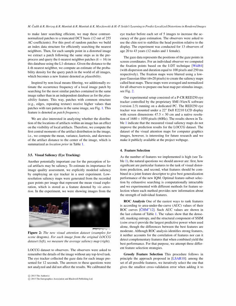
3.5. Visual Saliency (Eye Tracking)

Another potentially important cue for the perception of lo-cal artifacts may be saliency. To estimate its importance forimage quality assessment, we explicitly modeled saliencyby employing an eye tracker in a user experiment. Low-resolution saliency maps were generated from the recordedgaze points per image that represent the mean visual explo-ration, which is stored as a feature denoted by vis atten-

tion. In the experiment, we were showing images from the

0.2 0.4 0.6 0.8 10

Figure 2: The new visual attention dataset (examples for

scene dragons). For each image from the original LOCCG

dataset (left), we measure the average saliency map (right).

LOCCG dataset to observers. The observers were asked toremember the details of the image without any top-level task.The eye tracker collected the gaze data for each image pre-sented for 12 seconds. The answers to these questions werenot analyzed and did not affect the results. We calibrated the

eye tracker before each set of 5 images to increase the ac-curacy of the gaze estimation. The observers were asked touse the chin rest to stabilize the head position relative to thedisplay. The experiment was conducted for 13 observers ofage 20 to 43 years (12 males and 1 female).

The gaze data represents the positions of the gaze points inscreen coordinates. For an individual observer we computedthe fixation points based on the I-DT technique [Wid84](with dispersion and duration equal to 100 pixels and 250 msrespectively). The fixation maps were blurred using a low-pass Gaussian filter (σ=20 pixels) to create the saliency mapscalled heat maps. These maps were averaged and normalizedfor all observers to prepare one heat map per stimulus image,see Fig. 2.

Our experimental setup consisted of a P-CR RED250 eyetracker controlled by the proprietary SMI iViewX software(version 2.5) running on a dedicated PC. The RED250 eyetracker was mounted under a 22" Dell E2210 LCD displaywith screen dimensions 47.5× 30 cm and a native resolu-tion of 1680×1050 pixels (60Hz). The results shown in Ta-ble 1 indicate that the measured visual saliency maps do notimprove the prediction results for the LOCCG dataset. Thedataset of the visual attention maps for computer graphicsimages, however, is interesting for future research and wemake it publicly available at the project webpage.

4. Feature Selection

As the number of features we implemented is high (see Ta-ble 1), the natural questions we should answer are: first, howsignificant are particular features to the task of visual distor-tions prediction, and second, what features should be com-bined in a joint feature descriptor to give best generalizationperformance of the new IQM. Optimal feature-subset selec-tion by exhaustive searching is computationally intractableand we experimented with different methods for feature se-lection where each method provides new information aboutthe strength of individual features.

ROC Analysis One of the easiest ways to rank featuresis according to area-under-the-curve (AUC) values of theirROC curves [CHM∗12]. Such AUC values are shown inthe last column of Table 1. The values show that the dense-sift, masking entropy, and the structural component of SSIM(ssim struct) provide the largest predictive power when usedalone, though the differences between the best features aremoderate. Although ROC analysis identifies strong features,it neither accounts for the correlation of features nor can itdetect complementary features that when combined yield thebest performance. For that purpose, we attempt three differ-ent feature selection strategies.

Greedy Feature Selection This procedure follows inprinciple the approach proposed in [LSAR10]: among theset of all possible features, we iteratively select the one thatgives the smallest cross-validation error when adding it to



the pool of selected features and training a classifier on it.The process is continued until adding new features to thepool does not improve the cross-validation error. Here, forclassification we use a non-linear support vector machine[CL11] with radial basis function (RBF) kernel with hyper-parameters optimized by a grid-search.

Decision Forests Another common approach for featureselection is to analyze decision trees [Bre01], which wealso use for our metric described in Section 5. Ensemblesof decision trees are natural candidates for feature selec-tion [Bre01, TBRT09] since they intrinsically perform fea-ture selection at each node of the tree. The expected fre-quency that a single feature is chosen for a split in a randomtree and the trees impurity reduction due to the node splitindicates the relative importance of that feature to the treemodel [TBRT09]. This type of feature selection differs fromthe others in the sense that it only provides an importanceweight of the scalar components of individual features.

Stacked Classifiers To this end, we also analyzed the im-portance of individual features by an embedded SVM clas-sifier with L1-regularization [BM98]. To analyze the non-linear discriminative power of individual features, we builda 2-level stack of classifiers [Bre96b] where the first levelconsists of k non-linear classifiers (SVM) [CL11], one foreach feature, that compute the artifact probability based ona single feature. These probability values are fed forwardas k independent input features to the second level, whichis a single linear classifier w2 ∈ R

k. The classifier w2 isthen trained on a disjoint training set using a SVM withL1-regularization, which results in a sparse vector w2 thatcan be interpreted as a joint feature importance – the higherthe absolute weight wi = |w2(i)|, i ∈ {1, ..,k} the more dis-criminative the ith feature. Using this procedure the averageweights computed on LOCCG dataset with leave-one-outcross-validation are shown in Table 1.

4.1. Feature Selection Results

All feature selection strategies produce a reasonable featuresub-set that generalizes well when tested with leave-one-outcross-validation on trained decision tree ensembles as shownin the last row of Table 1. Although, the ROC analysis doesnot exploit correlation of features and selects only the best1-dimensional features the resulting combined feature sub-set is still performing well. However, when comparing thefeature scores (last 4 columns in Table 1) one can observesome discrepancies in the selected feature sets, which re-sult from slightly different objectives of the methods andcorrelation among the features. For example decision treescan be considered as ensembles of many weak classifiersbased on scalar features, whereas the greedy and the stack-ing approach operate on multi-dimensional features, and theROC analysis ignores feature combinations altogether. Fur-ther, correlation among individual features can produce dif-ferent sets that, when carefully observed, may actually be

0 20 40 60 80 1000

0.02

0.04

0.06

0.08

number of grown trees

clas

sific

atio

ner

ror

topt

10−1

100

101

0.02

0.04

0.06

0.08

quadratic error tolerance per node

cros

s−va

lidat

eder

ror

qe_opt

Figure 3: Optimal parameters of the decision forest. Left:

classification error versus number of decision trees t. Right:

optimal splitting threshold qe based on cross-validation.

similar. An example are the features hog9 diff and dense-siftdiff, which are highly correlated and chosen mutually exclu-sively by either method. Also, the signed difference (diff )is highly correlated with ad and is also a linear combina-tion of lum test and lum ref and therefore not selected inthe greedy approach but for the stacking and decision forest.Nevertheless, in agreement with the majority of the meth-ods, the SSIM structure component (ssim struc), the bag-of-words (bow), the masking entropy (mask. entropy I/II), andthe signed difference at multiple image scales (diff ) can beconsidered as important features for our task of classifyingdistortions. Further, we can also rule out certain features thateither do not improve performance or are simply redundant.These include absolute difference (ad), global image statis-tics (global stats), location of artifacts (location prior), andvisual attention (vis attention). In particular, all high-leveland global visual features (Section 3.4) perform rather weakin our analysis. However, this does not necessarily concludetheir ineffectiveness but rather our too simplistic modelingof the complex high-level human vision.

5. Data-Driven Metric

We experimented with different classification methods in-cluding Naive Bayes classifiers, linear and non-linear sup-port vector machines [CL11], and decision trees [Bre01].For our data-driven metric we obtained the best results (interms of ROC area-under-curve) with ensembles of baggeddecision trees [Bre01], which we refer to as decision for-

est. Decision forest is a powerful classification and regres-sion tool that is scalable and known for its robustness tonoise. Having constructed several random trees by boot-strapping [Bre96a], an observation is classified by traversingeach tree from root node to a leaf, which contains the pre-dicted label (artifact/no-artifact) that is averaged across alltrees. The path through the tree is determined by comparingsingle sub-features against learned thresholds in each node.The pruned tree depth and the number of trees controls theaccuracy of the classification. Using a cross-validation pro-tocol we empirically set the number of trees to t = 20 and theaverage tree depth to 10 (implicitly controlled by a quadraticerror tolerance threshold qe = 0.25 for the node-splitting),which yields good generalization performance (see Fig. 3).We train our metric using the 10 best features as derived inSection 4 (shown in the last but one column of Table 1).



0 0.1 0.2 0.3 0.4 0.5 0.6 0.7 0.8 0.9 10

0.1

0.2

0.3

0.4

0.5

0.6

0.7

0.8

0.9

1

False positive rate

Tru

e po

sitiv

e ra

te

rand

newMetric

SSIM

HDR−VDP−2

MS−SSIM

AD

sCIE−Lab

sCorrel

NoRM

0 0.1 0.2 0.3 0.4 0.5 0.6 0.7 0.8 0.9 1−0.2

0

0.2

0.4

0.6

0.8

Mat

thew

s co

rrel

atio

n

True positive rate

0.65 0.7 0.75 0.8 0.85 0.9

100% 57%

100%

68%

75%

76%

88%

78%

93%

69%

90%

85%

94%

NoRM

sCIE−Lab

MS−SSIM

HDR−VDP−2

AD

SSIM

sCorrel

newMetric

auc − area under curve

Figure 4: Quantitative results for quality metrics on

LOCCG dataset shown as ROC (top left) and Matthews cor-

relation (top right). The bigger the area under the curve

(AUC), the better. AUCnewMetric=0.916, AUCSSIM=0.858,

AUCHDRVDP2=0.802, AUCMSSSIM=0.786, AUCAD=0.832,

AUCsCIELab= 0.783, AUCsCorrel=0.880, AUCNoRM=0.644.

Bottom: ranking according to AUC (the percentages indi-

cate how often the metric on the right results in higher AUC

when the image set is randomized using a bootstrapping pro-

cedure similar to [CHM∗12]).

5.1. Results

We train our new data-driven metric described above onthe LOCCG dataset, which consists of 35 annotated image-pairs that exhibit a variety of computer graphics distortionsthat are difficult to predict by existing FR IQMs [CHM∗12].Since the size of the LOCCG dataset is rather small and theimages are very diverse showing (combination of) differentartifacts and scenes, we do not split it into a train and test set.We instead evaluate our method in a leave-one-out cross val-idation fashion; i.e., we train it on n− 1 images and test onthe n-th image repeating this process n times. In addition, wevalidate our metric on a new uncorrelated dataset that is de-scribed in Section 5.1.1. We compare the trained metric to 7state-of-the-art and baseline methods as shown in the quan-titative analysis in Fig. 4. Our new metric outperforms allexisting FR IQMs on the LOCCG dataset in terms of AUCin Fig. 4 (the higher the AUC the better). Also, the visual re-sults agree with the ground-truth annotation as shown in thecolor-coded distortion maps for three images of the LOCCGdataset in Fig. 5. Please refer to the supplementary materialfor all results and a more detailed analysis.

For completeness, we include results of the NR metricNoRM. However, this method was not originally intended tobe used for detecting general, mixed image distortions and istuned for only specific artifacts assuming the depth maps andother cues of the scenes to be available for feature computa-tion. Unfortunately, depth and texture maps are not availablein many cases in the LOCCG dataset, and we run NoRMonly with color features rendering its performance poor.

We implemented our new metric and feature computation

in MATLAB for which the code is available at the projectwebpage. Reporting the overall computation time of the un-optimized MATLAB code, the data preprocessing and fea-ture computation time per image (800×600) is in the orderof a few minutes, the time for training the decision forest onour selected feature set based on 100.000 samples takes lessthan 1 minute, whereas the distortion prediction using ourtrained decision forest requires only ≈ 0.5 sec.

5.1.1. Results for New Synthetic Dataset

Even though we report the result for cross validation to avoidover-training, we may expect that some distortions appear-ing in different images are correlated and the metric justlearns the distortions that are specific for that data set. Totest against this possibility, we measured another dataset.

The new Contrast-Luminance-Frequency-Masking(CLFM) dataset was measured using a similar procedureas in [CHM∗12]. 13 observers provided localized markingsfor the visible differences in 14 image pairs. The datasetwas designed to cover a wide range of problematic casesfor image quality assessment in possibly few images. Suchproblematic cases included increments of different sizeand contrast, edges shown at different luminance levels,random noise patterns of different frequency and contrast,several cases of contrast masking, image pairs with pixelmisalignment and noise patterns generated with a differentseed for the test and reference image (see example stimuliin Fig. 6). The CLFM dataset is available at the projectwebpage.

Fig. 7 shows the result of the tested metrics for the newdataset. Note that our new metric was trained on the LOCCGdataset and none of the new dataset images was used fortraining. From the shape of the ROC curves, it is clear thatthe CLFM dataset is extremely challenging and the metricsmispredict in many cases. But it is interesting to notice that,on average, the proposed metric has the highest AUC value.

Figure 6: CLFM: our synthetic validation dataset for test-

ing of IQMs perceptual-masking prediction. Top row: test

images containing (from left to right) increments of different

size, edges at different luminance levels, and band-limited

noise patterns organized in a CSF-like chart. Bottom: sub-

jective data for the corresponding images. (Best viewed in

electronic version.)



Figure 5: Comparison of distortion maps predicted by the proposed method with the state-of-the-art metrics for the red kitchen,and sponza tree shadows scenes. From left: subjective ground-truth, prediction of the new metric, SSIM, HDR-VDP-2, and

sCorrel. Please see the complete set of results in the supplementary material.

The performance expressed as Matthew’s correlation coef-ficient is very steady throughout the range of true positiverates, while many other metrics exhibit significant “dips”.This means that the new metric is less prone to loss of per-formance in the worst-case scenario.

It is encouraging to observe that learning the “real-world”distortions (e.g. based on the LOCCG dataset) may enabledecent prediction performance even for the synthetic datasetlike CLFM. This is different from the “traditional” approachto modeling quality metrics, where the synthetic cases areused to train the metric and the assumption is made thatthese will generalize for complex “real-world” cases. Inter-estingly, this correlates with our experience – when we usedsynthethic CLFM data for training, it did not lead to betterpredictions of LOCCG than traditional metrics.

6. Optimizing Existing Metrics

The stack of classifiers described in the last paragraph ofSection 4 can be used to optimize the parameters of tradi-tional metrics for the testing datasets. We show the resultsfor two metrics (SSIM and HDR-VDP-2) on the LOCCGdataset as an illustration of this approach.

0 0.1 0.2 0.3 0.4 0.5 0.6 0.7 0.8 0.9 10

0.1

0.2

0.3

0.4

0.5

0.6

0.7

0.8

0.9

1

False positive rate

Tru

e po

sitiv

e ra

te

rand

newMetric

SSIM

HDR−VDP−2

MS−SSIM

AD

sCIE−Lab

sCorrel

0 0.1 0.2 0.3 0.4 0.5 0.6 0.7 0.8 0.9 1−0.2

0

0.2

0.4

0.6

0.8

Mat

thew

s co

rrel

atio

n

True positive rate

Figure 7: Quantitative results for the new syn-

thetic dataset (CLFM) for our metric trained on the

LOCCG dataset. AUCnewMetric=0.805, AUCSSIM=0.695,

AUCHDRVDP2=0.772, AUCMSSSIM=0.714, AUCAD=0.733,

AUCsCIELab=0.763, AUCsCorrel=0.624.

6.1. Training SSIM

The stucture similarity metric (SSIM) consists of 3 termsthat were introduced in Eq. (1). The sensitivity or importanceof the individual terms is controlled by the parameters α, β,and γ, which are set to 1 by default.

We optimize those 3 parameters on the LOCCG datasetwith cross-validation to give the best possible prediction byemploying a linear support vector machine [CL11] that com-putes the optimal 3D weight vector w= [α∗

,β∗,γ∗]T for the

3 SSIM terms in the log domain log(SSIM∗)= α∗ · log(l)+β∗ · log(c)+γ∗ · log(s) =wT ·dlcs by minimizing the convexobjective function:

argminw

∑i

max(0,1− yi ·wT ·dlcsi )2+λ‖w‖22, (3)

where yi are the ground-truth labels in the dataset that are setto−1 or 1 if the distortion for the i-th training sample is vis-ible or not, respectively, and dlcsi ∈ R

3 is the correspondingprecomputed vector of the SSIM terms. The regularizationis controlled with λ = 1.

0.2 0.4 0.6 0.8 10

Figure 8: An illustration of the features of SSIM for the salascene where darker pixels represent more visible distortions.

From left: luminance, contrast, and structure term.

We run this optimization 35 times with randomized setof input images to assess the stability and quality of thecoefficients obtained. Interestingly, the results (Fig. 9, left)show a clear tendency towards higher weighting of the struc-ture and contrast components than the luminance compo-nent (α = 0.2, β = 2.8, γ = 3.5). This implies that thestructural and contrast components are more important thanthe luminance for computer graphics artifacts, which agrees



with the results presented in Section 4. Please notice thatthe performance improvement of the new weighted metric(SSIMlearned) compared to the original SSIM in Fig. 10. Anillustration of improvement of the distortion maps is shownin Fig. 11.

Figure 9: The results of the optimization of SSIM (left) and

HDR-VDP-2 (right) metric parameters. The red mark is the

median, the edges of the box are the 25th and 75th per-

centiles, the whiskers extend to extreme data points not con-

sidered outliers, and outliers are plotted individually. The

notches show 5% level intervals of the median significance.

6.2. Training HDR-VDP-2

Visible differences predictor for high-dynamic-range images(HDR-VDP-2) [MKRH11] is a perceptual metric that mod-els low-level human vision mechanisms, such as light adap-tation, spatial contrast sensitivity and contrast masking. Thepredicted probability of detecting differences between testand reference images is modeled as psychophysical detec-tion task separately for each spatial frequency band. Thecumulative probability is computed as probability summa-tion, which corresponds to summing logarithms of probabil-ity values from all bands. To introduce learning componentto the HDR-VDP-2, we weighted the logarithmic probabili-ties before summation. After learning, which used the identi-cal method as for the SSIM (Section 6.1), we found the opti-mum band weights to be (in decreasing frequency): w1=6.2,w2=12.1, w3=14.2, w4=9.6, w5=1.7, w6=10.2 (Fig. 9, right).Please notice the significant performance gain of the newweighted metric (HDR-VDP-2learned) compared to the orig-inal HDR-VDP-2 in Fig. 10. The improved distortion mapscan be found in Fig. 11.

7. Conclusions and Future Work

In this work we proposed a novel data-driven full-referenceimage quality metric, which outperforms existing IQMs indetecting perceivable rendering artifacts and reporting theirlocation in a distortion map. The key element of our met-ric is a carefully designed set of features, which general-ize over distortion types, image content, and superpositionof multiple distortions in a single image. We also proposeeasy to use customizations of existing metrics SSIM andHDR-VDP-2 that improve their performance in predictingrendering artifacts. Finally, as the outcome of this worktwo new datasets have been created, which are potentially

0 0.1 0.2 0.3 0.4 0.5 0.6 0.7 0.8 0.9 10

0.1

0.2

0.3

0.4

0.5

0.6

0.7

0.8

0.9

1

False positive rate

Tru

e po

sitiv

e ra

te

rand

newMetric

SSIM

HDR−VDP−2

SSIM_learned

HDR−VDP−2_learned

0 0.1 0.2 0.3 0.4 0.5 0.6 0.7 0.8 0.9 1−0.2

0

0.2

0.4

0.6

0.8

Mat

thew

s co

rrel

atio

n

True positive rate

Figure 10: Comparison of the overall results of op-

timized and original SSIM and HDR-VDP-2 met-

rics. Left: ROC, right: Matthews correlations. The

bigger the area under the ROC curve (AUC),

the better. AUCSSIM=0.858, AUCSSIMlearned=0.872,

AUCHDRVDP2=0.802, AUCHDRVDP2learned=0.883. The

result of newMetric (red) is shown here for comparison.

useful for the imaging and computer graphics communi-ties. The Contrast-Luminance-Frequency-Masking (CLFM)dataset contains a continuous range of basic distortions en-capsulated in a few images, with the distortion visibility an-notated in a perceptual experiment. The distortion saliencymaps captured in the eye tracking experiment could be usedfor further studies on visual attention, for example as a func-tion of rendering distortion type and its magnitude.

The main limitation of our work is the size of the trainingdataset, and we expect that the performance of our metriccan be still improved when a larger dataset is available. Fur-thermore, it would be interesting to explore other supervisedlearning techniques, e.g. [GRHS04], both for feature selec-tion and for FR metric prediction. The eye-tracking featuresdeserve further exploration too: for example the combinationof eye-tracking data with other features like absolute differ-ence could indicate where people gaze due to severe artifact.

Acknowledgements

This work was partially supported by the Polish Ministry of Scienceand Higher Education through the grant no. N N516 508539, and bythe COST Action IC1005 on “HDRi: The digital capture, storage,transmission and display of real-world lighting”.

References

[BM98] BRADLEY P. S., MANGASARIAN O. L.: Feature se-lection via concave minimization and support vector machines.In Proc. of 13th International Conference on Machine Learning

(1998), pp. 82–90. 6

[Bre96a] BREIMAN L.: Bagging Predictors. Machine Learning

24, 2 (Aug. 1996), 123–140. 6

[Bre96b] BREIMAN L.: Stacked regressions. Machine Learning

24 (1996), 49–64. 6

[Bre01] BREIMAN L.: Random forests. Machine Learning 45, 1(2001), 5–32. 6



Figure 11: An example of the improved predictions of SSIM and HDR-VDP-2 for the sponza above tree scene after the param-eter optimization. From left: subjective ground-truth, prediction of SSIM, SSIMlearned, HDR-VDP-2, HDR-VDP-2learned.

[BZM07] BOSCH A., ZISSERMAN A., MUNOZ X.: Image clas-sifcation using random forests and ferns. In Proc. of ICCV

(2007), 1–8. 3, 4

[CHM∗12] CADÍK M., HERZOG R., MANTIUK R.,MYSZKOWSKI K., SEIDEL H.-P.: New measurements re-veal weaknesses of image quality metrics in evaluating graphicsartifacts. ACM TOG (Proc. of SIGGRAPH 2012) (2012). Article147. 1, 2, 3, 4, 5, 7

[CL11] CHANG C.-C., LIN C.-J.: LIBSVM: A library for sup-port vector machines. ACM Transactions on Intelligent Systems

and Technology 2 (2011), 27:1–27:27. 6, 8

[DT05] DALAL N., TRIGGS B.: Histograms of oriented gradientsfor human detection. Proc. of IEEE Computer Vision and Pattern

Recognition (2005), 886–893. 3, 4

[FFP05] FEI-FEI L., PERONA P.: A bayesian hierarchical modelfor learning natural scene categories. Proc. of IEEE Computer

Vision and Pattern Recognition (2005), 524–531. 4

[GRHS04] GOLDBERGER J., ROWEIS S., HINTON G.,SALAKHUTDINOV R.: Neighbourhood components analy-sis. In Advances in Neural Information Processing Systems 17

(2004), MIT Press, pp. 513–520. 9

[HCA∗12] HERZOG R., CADÍK M., AYDIN T. O., KIM K. I.,MYSZKOWSKI K., SEIDEL H.-P.: NoRM: no-reference imagequality metric for realistic image synthesis. Computer GraphicsForum 31, 2 (2012), 545–554. 2

[HS88] HARRIS C., STEPHENS M.: A combined corner and edgedetector. Proc. of the 4th Alvey Vision Conference (1988), 147–151. 3, 4

[Kov99] KOVESI P.: Image features from phase congruency.Videre: A Journal of Computer Vision Research 1, 3 (1999). 3, 4

[LBW11] LI C., BOVIK A. C., WU X.: Blind image quality as-sessment using a general regression neural network. IEEE Trans-

actions on Neural Networks 22, 5 (2011), 793–9. 2

[LSAR10] LIU C., SHARAN L., ADELSON E., ROSENHOLTZ

R.: Exploring features in a bayesian framework for materialrecognition. Proc. of IEEE Computer Vision and Pattern Recog-

nition (2010), 239–246. 5

[Lub95] LUBIN J.: Vision Models for Target Detection and

Recognition. ed. E. Peli. World Scientific, 1995, ch. A VisualDiscrimination Model for Imaging System Design and Evalua-tion, pp. 245–283. 1

[MB10] MOORTHY A., BOVIK A.: A two-step framework forconstructing blind image quality indices. IEEE Signal Processing

Letters 17, 5 (2010), 513 –516. 2

[MKRH11] MANTIUK R., KIM K. J., REMPEL A. G., HEI-DRICH W.: HDR-VDP-2: a calibrated visual metric for visibilityand quality predictions in all luminance conditions. ACM TOG

(Proc. of SIGGRAPH 2011) (2011). Article 40. 1, 2, 3, 9

[NL10] NARWARIA M., LIN W.: Objective image quality assess-ment based on support vector regression. IEEE Transactions on

Neural Networks 21, 3 (2010), 515–9. 2

[PH11] PEDERSEN M., HARDEBERG J.: Full-reference imagequality metrics: Classification and evaluation. Found. Trends.

Comput. Graph. Vis. 7, 1 (2011), 1–80. 1, 2

[RFWB07] RAMANARAYANAN G., FERWERDA J., WALTER B.,BALA K.: Visual equivalence: towards a new standard for imagefidelity. ACM TOG (Proc. of SIGGRAPH 2007) (2007). 2

[RGHZ10] REDI J. A., GASTALDO P., HEYNDERICKX I.,ZUNINO R.: Color distribution information for the reduced-reference assessment of perceived image quality. IEEE Trans. on

Circuits and Systems for Video Techn. 20, 12 (2010), 1757–69. 2

[RTMF07] RUSSELL B., TORRALBA A., MURPHY K., FREE-MAN W. T.: Labelme: a database and web-based tool for imageannotation. International Journal of Computer Vision (2007). 4

[SBC05] SHEIKH H., BOVIK A., CORMACK L.: No-referencequality assessment using natural scene statistics: JPEG2000.IEEE Trans. on Image Processing 14, 11 (2005), 1918–1927. 2

[SBC10] SAAD M., BOVIK A., CHARRIER C.: A DCT statistics-based blind image quality index. IEEE Signal Processing Letters

17, 6 (2010), 583 –586. 2

[SSB06] SHEIKH H., SABIR M., BOVIK A.: A statistical evalua-tion of recent full reference image quality assessment algorithms.IEEE Trans. on Image Processing 15, 11 (2006), 3440–3451. 1

[SWCB06] SHEIKH H. R., WANG Z., CORMACK L., BOVIK

A. C.: LIVE image quality assessment database RLS 2, 2006.2, 4

[TBRT09] TUV E., BORISOV A., RUNGER G., TORKKOLA K.:Feature selection with ensembles, artificial variables, and redun-dancy elimination. Journal of Machine Learning Research 10

(2009), 1341–1366. 6

[TJK11] TANG H., JOSHI N., KAPOOR A.: Learning a blindmeasure of perceptual image quality. Proc. of IEEE Computer

Vision and Pattern Recognition (2011), 305–312. 2

[TM08] TUYTELAARS T., MIKOLAJCZYK K.: Local invariantfeature detectors: a survey. Found. Trends. Comput. Graph. Vis.3, 3 (2008), 177–280. 2, 3

[WB06] WANG Z., BOVIK A. C.: Modern Image Quality Assess-

ment. Morgan & Claypool Publishers, 2006. 1, 2, 3

[WBSS04] WANG Z., BOVIK A. C., SHEIKH H. R., SIMON-CELLI E. P.: Image quality assessment: From error visibilityto structural similarity. IEEE Trans. on Image Processing 13, 4(2004), 600–612. 3, 4

[Wid84] WIDDEL H.: Operational problems in analysing eyemovements. In A.G. Gale & F. Johnson (Eds.), Theoretical and

Applied Aspects of Eye Movement Research. 1 (1984), 21–29. 5

[ZW97] ZHANG X., WANDELL B. A.: A spatial extension ofCIELAB for digital color-image reproduction. Journal of the So-ciety for Information Display 5, 1 (1997), 61. 3


learning to predict localized distortions in rendered …rkm38/pdfs/cadik13learning.pdf · learning...

Documents