learning to adapt structured output space for semantic ... · learning to adapt structured output...

Learning to Adapt Structured Output Space for Semantic Segmentation

Yi-Hsuan Tsai1∗ Wei-Chih Hung2∗ Samuel Schulter1 Kihyuk Sohn1

Ming-Hsuan Yang2 Manmohan Chandraker11NEC Laboratories America 2University of California, Merced

Abstract

Convolutional neural network-based approaches for se-mantic segmentation rely on supervision with pixel-levelground truth, but may not generalize well to unseen imagedomains. As the labeling process is tedious and labor inten-sive, developing algorithms that can adapt source groundtruth labels to the target domain is of great interest. In thispaper, we propose an adversarial learning method for do-main adaptation in the context of semantic segmentation.Considering semantic segmentations as structured outputsthat contain spatial similarities between the source and tar-get domains, we adopt adversarial learning in the outputspace. To further enhance the adapted model, we con-struct a multi-level adversarial network to effectively per-form output space domain adaptation at different featurelevels. Extensive experiments and ablation study are con-ducted under various domain adaptation settings, includ-ing synthetic-to-real and cross-city scenarios. We show thatthe proposed method performs favorably against the state-of-the-art methods in terms of accuracy and visual quality.

1. IntroductionSemantic segmentation aims to assign each pixel a se-

mantic label, e.g., person, car, road or tree, in an image.Recently, methods based on convolutional neural networks(CNNs) have achieved significant progress in semantic seg-mentation [2, 21, 23, 24, 40, 42, 43] with applications forautonomous driving [9] and image editing [36]. The cruxof CNN-based approaches is to annotate a large number ofimages that cover possible scene variations. However, thistrained model may not generalize well to unseen images,especially when there is a domain gap between the training(source) and test (target) images. For instance, the distribu-tion of appearance for objects and scenes may vary in dif-ferent cities, and even weather and lighting conditions canchange significantly in the same city. In such cases, rely-

∗Both authors contribute equally to this work.

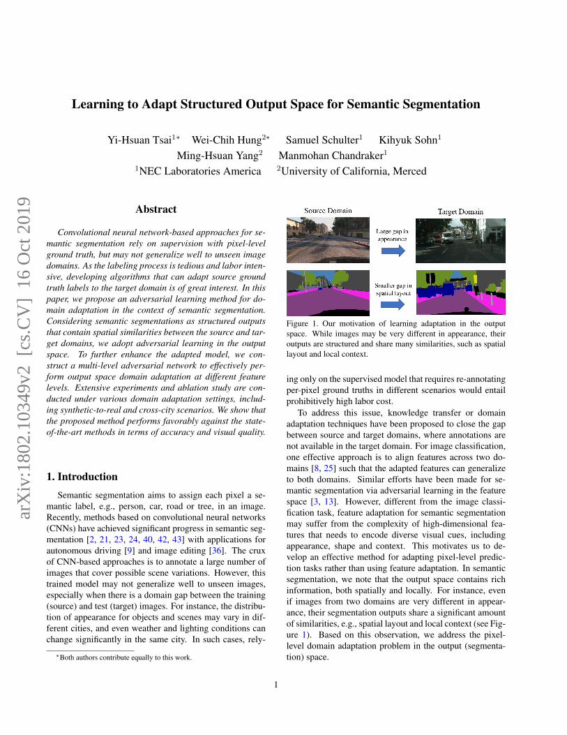
Figure 1. Our motivation of learning adaptation in the outputspace. While images may be very different in appearance, theiroutputs are structured and share many similarities, such as spatiallayout and local context.

ing only on the supervised model that requires re-annotatingper-pixel ground truths in different scenarios would entailprohibitively high labor cost.

To address this issue, knowledge transfer or domainadaptation techniques have been proposed to close the gapbetween source and target domains, where annotations arenot available in the target domain. For image classification,one effective approach is to align features across two do-mains [8, 25] such that the adapted features can generalizeto both domains. Similar efforts have been made for se-mantic segmentation via adversarial learning in the featurespace [3, 13]. However, different from the image classi-fication task, feature adaptation for semantic segmentationmay suffer from the complexity of high-dimensional fea-tures that needs to encode diverse visual cues, includingappearance, shape and context. This motivates us to de-velop an effective method for adapting pixel-level predic-tion tasks rather than using feature adaptation. In semanticsegmentation, we note that the output space contains richinformation, both spatially and locally. For instance, evenif images from two domains are very different in appear-ance, their segmentation outputs share a significant amountof similarities, e.g., spatial layout and local context (see Fig-ure 1). Based on this observation, we address the pixel-level domain adaptation problem in the output (segmenta-tion) space.

1

arX

iv:1

802.

1034

9v2

[cs

.CV

] 1

6 O

ct 2

019

In this paper, we propose an end-to-end CNN-based do-main adaptation algorithm for semantic segmentation. Ourformulation is based on adversarial learning in the outputspace, where the intuition is to directly make the predictedlabel distributions close to each other across source and tar-get domains. Based on the generative adversarial network(GAN) [10, 31, 22], the proposed model consists of twoparts: 1) a segmentation model to predict output results, and2) a discriminator to distinguish whether the input is fromthe source or target segmentation output. With an adversar-ial loss, the proposed segmentation model aims to fool thediscriminator, with the goal of generating similar distribu-tions in the output space for either source or target images.

The proposed method also adapts features as the errorsare back-propagated to the feature level from the output la-bels. However, one concern is that lower-level features maynot be adapted well as they are far away from the high-leveloutput labels. To address this issue, we develop a multi-level strategy by incorporating adversarial learning at differ-ent feature levels of the segmentation model. For instance,we can use both conv5 and conv4 features to predict seg-mentation results in the output space. Then two discrimi-nators can be connected to each of the predicted output formulti-level adversarial learning. We perform one-stage end-to-end training for the segmentation model and discrimina-tors jointly, without using any prior knowledge of the data inthe target domain. In the testing phase, we can simply dis-card discriminators and use the adapted segmentation modelon target images, with no extra computational requirements.

Due to the high labor cost of annotating segmentationground truth, there has been great interest in large-scale syn-thetic datasets with annotations, e.g., GTA5 [32] and SYN-THIA [33]. As a result, one critical setting is to adapt themodel trained on synthetic data to real-world datasets, suchas Cityscapes [4]. We follow this setting and conduct ex-tensive experiments to validate the proposed domain adap-tation method. First, we use a strong baseline model thatis able to generalize to different domains. We note that astrong baseline facilitates real-world applications and canevaluate the limitation of the proposed adaptation approach.Based on this baseline model, we show comparisons usingadversarial adaptation in the feature and output spaces. Fur-thermore, we show that the multi-level adversarial learningimproves the results over single-level adaptation. In addi-tion to the synthetic-to-real setting, we show experimentalresults on the Cross-City dataset [3], where annotations areprovided in one city (source), while testing the model onanother unseen city (target). Overall, our method performsfavorably against state-of-the-art algorithms on numerousbenchmark datasets under different settings.

The contributions of this work are as follows. First,we propose a domain adaptation method for pixel-level se-mantic segmentation via adversarial learning. Second, we

demonstrate that adaptation in the output (segmentation)space can effectively align scene layout and local contextbetween source and target images. Third, a multi-level ad-versarial learning scheme is developed to adapt features atdifferent levels of the segmentation model, which leads toimproved performance.

2. Related WorkSemantic Segmentation. State-of-the-art semantic seg-mentation methods are mainly based on the recent advancesof deep neural networks. As proposed by Long et al. [24],one can transform a classification CNN (e.g., AlexNet [19],VGG [34], or ResNet [11]) to a fully-convolutional net-work (FCN) for semantic segmentation. Numerous meth-ods have since been developed to improve this model byutilizing context information [15, 42] or enlarging receptivefields [2, 40]. To train these advanced networks, a substan-tial amount of dense pixel annotations must be collected inorder to match the model capacity of deep CNNs. As a re-sult, weakly and semi-supervised approaches [5, 14, 17, 29,30] are proposed in recent years to reduce the heavy label-ing cost of collecting segmentation ground truths. However,in most real-world applications, it is difficult to obtain weakannotations and the trained model may not generalize wellto unseen image domains.

Another approach to tackle the annotation problem isto construct synthetic datasets based on rendering, e.g.,GTA5 [32] and SYNTHIA [33]. While the data collectionis less costly since the pixel-level annotation can be donewith a partially automated process, these datasets are usu-ally used in conjunction with real-world datasets for jointlearning to improve the performance. However, when train-ing solely on the synthetic dataset, the model does not gen-eralize well to real-world data, mainly due to the large do-main shift between synthetic images and real-world images,i.e., appearance differences are still significant with currentrendering techniques. Although synthesizing more realisticimages can decrease the domain shift, it is necessary to usedomain adaptation to narrow the performance gap.

Domain Adaptation. Domain adaptation methods forimage classification have been developed to address thedomain-shift problem between the source and target do-mains. Numerous methods [7, 8, 25, 26, 35, 37, 38] are de-veloped based on CNN classifiers due to performance gain.The main insight behind these approaches is to tackle theproblem by aligning the feature distribution between sourceand target images. Ganin et al. [7, 8] propose the Domain-Adversarial Neural Network (DANN) to transfer the featuredistribution. A number of variants have since been proposedwith different loss functions [25, 37, 38] or classifiers [26].Recently, the PixelDA method [1] addresses domain adap-tation for image classification by transferring the source im-

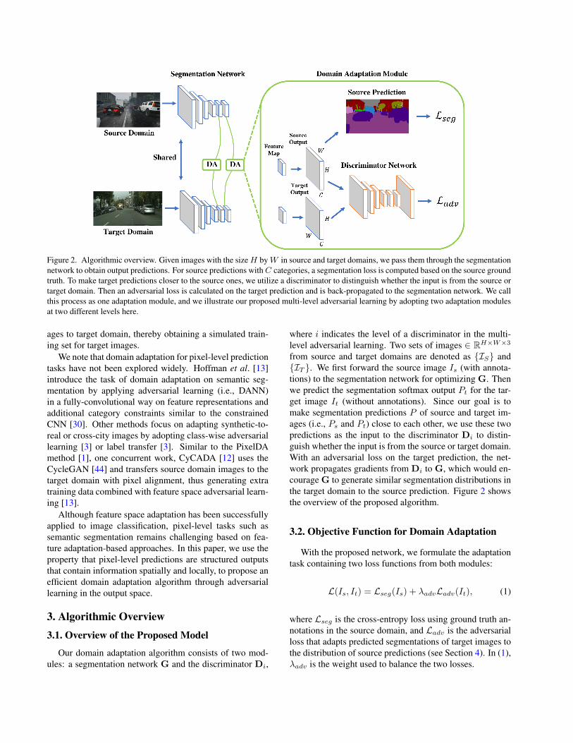
Figure 2. Algorithmic overview. Given images with the sizeH byW in source and target domains, we pass them through the segmentationnetwork to obtain output predictions. For source predictions withC categories, a segmentation loss is computed based on the source groundtruth. To make target predictions closer to the source ones, we utilize a discriminator to distinguish whether the input is from the source ortarget domain. Then an adversarial loss is calculated on the target prediction and is back-propagated to the segmentation network. We callthis process as one adaptation module, and we illustrate our proposed multi-level adversarial learning by adopting two adaptation modulesat two different levels here.

ages to target domain, thereby obtaining a simulated train-ing set for target images.

We note that domain adaptation for pixel-level predictiontasks have not been explored widely. Hoffman et al. [13]introduce the task of domain adaptation on semantic seg-mentation by applying adversarial learning (i.e., DANN)in a fully-convolutional way on feature representations andadditional category constraints similar to the constrainedCNN [30]. Other methods focus on adapting synthetic-to-real or cross-city images by adopting class-wise adversariallearning [3] or label transfer [3]. Similar to the PixelDAmethod [1], one concurrent work, CyCADA [12] uses theCycleGAN [44] and transfers source domain images to thetarget domain with pixel alignment, thus generating extratraining data combined with feature space adversarial learn-ing [13].

Although feature space adaptation has been successfullyapplied to image classification, pixel-level tasks such assemantic segmentation remains challenging based on fea-ture adaptation-based approaches. In this paper, we use theproperty that pixel-level predictions are structured outputsthat contain information spatially and locally, to propose anefficient domain adaptation algorithm through adversariallearning in the output space.

3. Algorithmic Overview

3.1. Overview of the Proposed Model

Our domain adaptation algorithm consists of two mod-ules: a segmentation network G and the discriminator Di,

where i indicates the level of a discriminator in the multi-level adversarial learning. Two sets of images ∈ RH×W×3

from source and target domains are denoted as {IS} and{IT }. We first forward the source image Is (with annota-tions) to the segmentation network for optimizing G. Thenwe predict the segmentation softmax output Pt for the tar-get image It (without annotations). Since our goal is tomake segmentation predictions P of source and target im-ages (i.e., Ps and Pt) close to each other, we use these twopredictions as the input to the discriminator Di to distin-guish whether the input is from the source or target domain.With an adversarial loss on the target prediction, the net-work propagates gradients from Di to G, which would en-courage G to generate similar segmentation distributions inthe target domain to the source prediction. Figure 2 showsthe overview of the proposed algorithm.

3.2. Objective Function for Domain Adaptation

With the proposed network, we formulate the adaptationtask containing two loss functions from both modules:

L(Is, It) = Lseg(Is) + λadvLadv(It), (1)

where Lseg is the cross-entropy loss using ground truth an-notations in the source domain, and Ladv is the adversarialloss that adapts predicted segmentations of target images tothe distribution of source predictions (see Section 4). In (1),λadv is the weight used to balance the two losses.

4. Output Space AdaptationDifferent from image classification based on features

[8, 25] that describe the global visual information of theimage, high-dimensional features learned for semantic seg-mentation encodes complex representations. As a result,adaptation in the feature space may not be the best choicefor semantic segmentation. On the other hand, althoughsegmentation outputs are in the low-dimensional space, theycontain rich information, e.g., scene layout and context. Ourintuition is that no matter images are from the source or tar-get domain, their segmentations should share strong simi-larities, spatially and locally. Thus, we utilize this propertyto adapt low-dimensional softmax outputs of segmentationpredictions via an adversarial learning scheme.

4.1. Single-level Adversarial LearningDiscriminator Training. Before introducing how to adaptthe segmentation network via adversarial learning, we firstdescribe the training objective for the discriminator. Giventhe segmentation softmax output P = G(I) ∈ RH×W×C ,where C is the number of categories, we forward P to afully-convolutional discriminator D using a cross-entropyloss Ld for the two classes (i.e., source and target). The losscan be written as:

Ld(P ) = −∑h,w

(1− z) log(D(P )(h,w,0)) (2)

+z log(D(P )(h,w,1)),

where z = 0 if the sample is drawn from the target domain,and z = 1 for the sample from the source domain.Segmentation Network Training. First, we define the seg-mentation loss in (1) as the cross-entropy loss for imagesfrom the source domain:

Lseg(Is) = −∑h,w

∑c∈C

Y (h,w,c)s log(P (h,w,c)

s ), (3)

where Ys is the ground truth annotations for source imagesand Ps = G(Is) is the segmentation output.

Second, for images in the target domain, we forwardthem to G and obtain the prediction Pt = G(It). To makethe distribution of Pt closer to Ps, we use an adversarial lossLadv in (1) as:

Ladv(It) = −∑h,w

log(D(Pt)(h,w,1)). (4)

This loss is designed to train the segmentation network andfool the discriminator by maximizing the probability of thetarget prediction being considered as the source prediction.

4.2. Multi-level Adversarial Learning

Although performing adversarial learning in the outputspace directly adapts predictions, low-level features may

not be adapted well as they are far away from the output.Similar to the deep supervision method [20] that uses aux-iliary loss for semantic segmentation [42], we incorporateadditional adversarial module in the low-level feature spaceto enhance the adaptation. The training objective for thesegmentation network can be extended from (1) as:

L(Is, It) =∑i

λisegLiseg(Is) +

∑i

λiadvLiadv(It), (5)

where i indicates the level used for predicting the segmen-tation output. We note that, the segmentation output isstill predicted in each feature space, before passing throughindividual discriminators for adversarial learning. Hence,Liseg(Is) and Li

adv(It) remain in the same form as in (3)and (4), respectively. Based on (5), we optimize the follow-ing min-max criterion:

maxD

minGL(Is, It). (6)

The ultimate goal is to minimize the segmentation loss inG for source images, while maximizing the probability oftarget predictions being considered as source predictions.

5. Network Architecture and TrainingDiscriminator. For the discriminator, we use an architec-ture similar to [31] but utilize all fully-convolutional lay-ers to retain the spatial information. The network consistsof 5 convolution layers with kernel 4 × 4 and stride of 2,where the channel number is {64, 128, 256, 512, 1}, re-spectively. Except for the last layer, each convolution layeris followed by a leaky ReLU [27] parameterized by 0.2. Anup-sampling layer is added to the last convolution layer forre-scaling the output to the size of the input. We do not useany batch-normalization layers [16] as we jointly train thediscriminator with the segmentation network using a smallbatch size.Segmentation Network. It is essential to build upon a goodbaseline model to achieve high-quality segmentation results[2, 40, 42]. We adopt the DeepLab-v2 [2] framework withResNet-101 [11] model pre-trained on ImageNet [6] as oursegmentation baseline network. However, we do not usethe multi-scale fusion strategy [2] due to the memory issue.Similar to the recent work on semantic segmentation [2, 40],we remove the last classification layer and modify the strideof the last two convolution layers from 2 to 1, making theresolution of the output feature maps effectively 1/8 timesthe input image size. To enlarge the receptive field, we ap-ply dilated convolution layers [40] in conv4 and conv5 lay-ers with a stride of 2 and 4, respectively. After the last layer,we use the Atrous Spatial Pyramid Pooling (ASPP) [2] asthe final classifier. Finally, we apply an up-sampling layeralong with the softmax output to match the size of the inputimage. Based on this architecture, our segmentation model

Table 1. Results of adapting GTA5 to Cityscapes. We first compare our results using single-level adversarial learning in the output spacewith other state-of-the-art algorithms with the VGG-16 based model. Then we adopt the ResNet-101 based model and present ablationstudy on different components of our proposed method.

GTA5 → Cityscapes

Method road

side

wal

k

build

ing

wal

l

fenc

e

pole

light

sign

veg

terr

ain

sky

pers

on

ride

r

car

truc

k

bus

trai

n

mbi

ke

bike

mIoU

FCNs in the Wild [13] 70.4 32.4 62.1 14.9 5.4 10.9 14.2 2.7 79.2 21.3 64.6 44.1 4.2 70.4 8.0 7.3 0.0 3.5 0.0 27.1CDA [41] 74.9 22.0 71.7 6.0 11.9 8.4 16.3 11.1 75.7 13.3 66.5 38.0 9.3 55.2 18.8 18.9 0.0 16.8 14.6 28.9CyCADA (feature) [12] 85.6 30.7 74.7 14.4 13.0 17.6 13.7 5.8 74.6 15.8 69.9 38.2 3.5 72.3 16.0 5.0 0.1 3.6 0.0 29.2CyCADA (pixel) [12] 83.5 38.3 76.4 20.6 16.5 22.2 26.2 21.9 80.4 28.7 65.7 49.4 4.2 74.6 16.0 26.6 2.0 8.0 0.0 34.8Ours (singel-level) 87.3 29.8 78.6 21.1 18.2 22.5 21.5 11.0 79.7 29.6 71.3 46.8 6.5 80.1 23.0 26.9 0.0 10.6 0.3 35.0

Baseline (ResNet) 75.8 16.8 77.2 12.5 21.0 25.5 30.1 20.1 81.3 24.6 70.3 53.8 26.4 49.9 17.2 25.9 6.5 25.3 36.0 36.6Ours (feature) 83.7 27.6 75.5 20.3 19.9 27.4 28.3 27.4 79.0 28.4 70.1 55.1 20.2 72.9 22.5 35.7 8.3 20.6 23.0 39.3Ours (single-level) 86.5 25.9 79.8 22.1 20.0 23.6 33.1 21.8 81.8 25.9 75.9 57.3 26.2 76.3 29.8 32.1 7.2 29.5 32.5 41.4Ours (multi-level) 86.5 36.0 79.9 23.4 23.3 23.9 35.2 14.8 83.4 33.3 75.6 58.5 27.6 73.7 32.5 35.4 3.9 30.1 28.1 42.4

achieves 65.1% mean intersection-over-union (IoU) whentrained on the Cityscapes [4] training set and tested on theCityscapes validation set.

Multi-level Adaptation Model. We construct the above-mentioned discriminator and segmentation network as oursingle-level adaptation model. For the multi-level structure,we extract feature maps from the conv4 layer and add anASPP module as the auxiliary classifier. Similarly, a dis-criminator with the same architecture is added for adversar-ial learning. Figure 2 shows the proposed multi-level adap-tation model. In this paper, we use two levels due to thebalance of its efficiency and accuracy.Network Training. To train the proposed single/multi-leveladaptation model, we find that jointly training the segmen-tation network and discriminators in one stage is effective.In each training batch, we first forward the source image Isto optimize the segmentation network for Lseg in (3) andgenerate the output Ps. For the target image It, we obtainthe segmentation output Pt, and pass it along with Ps to thediscriminator for optimizingLd in (2). In addition, we com-pute the adversarial loss Ladv in (4) for the target predictionPt. For the multi-level training objective in (5), we simplyrepeat the same procedure for each adaptation module.

We implement our network using the PyTorch toolboxon a single Titan X GPU with 12 GB memory. To trainthe segmentation network, we use the Stochastic GradientDescent (SGD) optimizer with Nesterov acceleration wherethe momentum is 0.9 and the weight decay is 10−4. Theinitial learning rate is set as 2.5 × 10−4 and is decreasedusing the polynomial decay with power of 0.9 as mentionedin [2]. For training the discriminator, we use the Adam op-timizer [18] with the learning rate as 10−4 and the samepolynomial decay as the segmentation network. The mo-mentum is set as 0.9 and 0.99.

Table 2. Performance gap between the adapted model and thefully-supervised (oracle) model. We first compare results withstate-of-the-art methods using the VGG based model, and thenshow our result using the ResNet one.

GTA5 → Cityscapes

method Baseline Adapt Oracle mIoU Gap

FCNs in the Wild [13]

VGG-16

27.1 64.6 -37.5CDA [41] 28.9 60.3 -31.4CyCADA (feature) [12] 29.2 60.3 -30.5CyCADA (pixel) [12] 34.8 60.3 -24.9Ours (single-level) 35.0 61.8 -25.2

Ours (multi-level) ResNet-101 42.4 65.1 -22.7

6. Experimental ResultsIn this section, we present experimental results to val-

idate the proposed domain adaptation method for seman-tic segmentation under different settings. First, we showevaluations of the model trained on synthetic datasets (i.e.,GTA5 [32] and SYNTHIA [33]) and test the adapted modelon real-world images from the Cityscapes [4] dataset. Ex-tensive experiments including comparisons to the state-of-the-art methods and ablation study are also conducted, e.g.,adaptation in the feature/output spaces and single/multi-level adversarial learning. Second, we carry out experi-ments on the Cross-City dataset [3], where the model istrained on one city and adapted to another city withoutusing annotations. In all the experiments, the IoU met-ric is used. The code and model are available at https://github.com/wasidennis/AdaptSegNet.

6.1. GTA5

The GTA5 dataset [32] consists of 24966 images withthe resolution of 1914 × 1052 synthesized from the video

https://github.com/wasidennis/AdaptSegNet

https://github.com/wasidennis/AdaptSegNet

game based on the city of Los Angeles. The ground truthannotations are compatible with the Cityscapes dataset [4]that contains 19 categories. Following [13], we use the fullset of GTA5 and adapt the model to the Cityscapes trainingset with 2975 images. During testing, we evaluate on theCityscapes validation set with 500 images.

Overall Results. We present adaptation results in Table 1with comparisons to the state-of-the-art domain adaptationmethods [12, 13, 41]. For these approaches, the baselinemodel is trained using VGG-based architectures [24, 40].To fairly evaluate our method, we first use the same baselinearchitecture (VGG-16) and train our model with the pro-posed single-level adaptation module. Table 1 shows thatour method performs favorably against the other algorithms.While these methods all have feature adaptation modules,our results show that adapting the model in the output spaceachieves better performance. We note that CyCADA [12]has a pixel adaptation module by transforming source do-main images to the target domain and hence obtains ad-ditional training samples. Although this strategy achievesa similar performance as ours, one can always apply pixeltransformation combined with our output space adaptationto improve the results.

On the other hand, we argue that utilizing a strongerbaseline model is critical for understanding the importanceof different adaptation components as well as for enhancingthe performance to enable real-world applications. Thus,we use the ResNet-101 based network introduced in Sec-tion 5 and train the proposed adaptation model. Table 1shows the baseline results only trained on source imageswithout adaptation, with comparisons to our adapted mod-els under different settings, including feature adaptation andsingle/multi-level adversarial learning in the output space.Figure 3 presents some example results for adapted seg-mentation. We note that for small objects such as poles andtraffic signs, they are harder to adapt since they easily getmerged with background classes.

In addition, another factor to evaluate the adaptation per-formance is to measure how much gap is narrowed be-tween the adaptation model and the fully-supervised model.Hence, we train the model using annotated ground truthsin the Cityscapes dataset as the oracle results. Table 2shows the gap under different baseline models. We observethat, although the oracle result does not differ a lot betweenVGG-16 and ResNet-101 based models, the gap is larger forthe VGG one. It suggests us that to narrow the gap, using adeeper model with larger capacity is more practical.Parameter Analysis. During optimizing the segmentationnetwork G, it is essential to balance the weight betweensegmentation and adversarial losses. We first consider thesingle-level case in (1) and conduct experiments to observethe impact of changing λadv . Table 3 shows that a smallerλadv may not facilitate the training process significantly,

Table 3. Sensitivity analysis of λadv for feature/output space do-main adaptation in the proposed method. We show that outputspace adaptation can tolerate a wide range of λadv , while it is sen-sitive to change λadv for feature adaptation.

GTA5 → Cityscapes

λadv 0.0005 0.001 0.002 0.004

Feature 35.3 39.3 35.9 32.8Output Space 40.2 41.4 40.4 40.1

while a larger λadv may propagate incorrect gradients tothe network. We empirically choose λadv as 0.001 in thesingle-level setting.Feature Level v.s. Output Space Adaptation. In thesingle-level setting in (1), we compare results by usingfeature-level or output space adaptation via adversariallearning. For feature-level adaptation, we adopt a similarstrategy as used in [13, 3] and train our model accordingly.Table 1 shows that the proposed adaptation method in theoutput space performs better than the one in the featurelevel.

In addition, Table 3 shows that adaptation in the featurespace is more sensitive to λadv , which causes the trainingprocess more difficult, while output space adaptation allowsfor a wider range of λadv . One reason is that as featureadaptation is performed in the high-dimensional space, theproblem for the discriminator becomes easier. Thus, suchan adapted model cannot effectively match distributions be-tween source and target domains via adversarial learning.

Single-level v.s. Multi-level Adversarial Learning. Wehave shown the merits of adopting adversarial learning inthe output space. In addition, we present the results of us-ing multi-level adversarial learning in Table 1. Here, weutilize an additional adversarial module (see Figure 2) andjointly optimize (5) for two levels. To properly balance λisegand λiadv , we use the same weight as in the single-level set-ting for the high-level output space (i.e., λ1seg = 1 and λ1adv= 0.001). Since the low-level output carries less informa-tion to predict the segmentation, we use smaller weights forboth the segmentation and adversarial loss (i.e., λ2seg = 0.1and λ2adv = 0.0002). Evaluation results show that our multi-level adversarial adaptation further improves the segmenta-tion accuracy. More results and analysis are presented inthe supplementary material.

6.2. SYNTHIA

To adapt from the SYNTHIA to Cityscapes datasets,we use the SYNTHIA-RAND-CITYSCAPES [33] set asthe source domain which contains 9400 images compati-ble with the cityscapes annotated classes. Similar to [3],we evaluate images on the Cityscapes validation set with 13

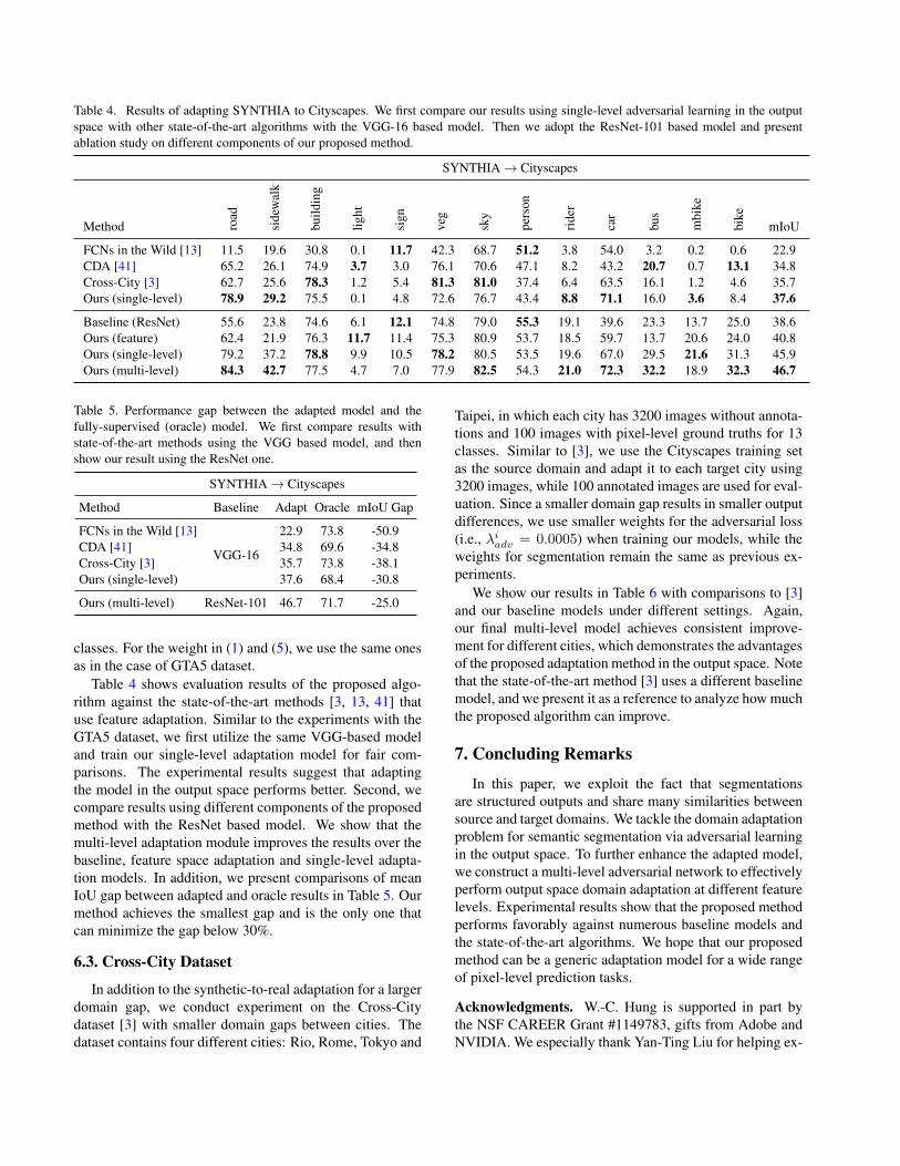
Table 4. Results of adapting SYNTHIA to Cityscapes. We first compare our results using single-level adversarial learning in the outputspace with other state-of-the-art algorithms with the VGG-16 based model. Then we adopt the ResNet-101 based model and presentablation study on different components of our proposed method.

SYNTHIA → Cityscapes

Method road

side

wal

k

build

ing

light

sign

veg

sky

pers

on

ride

r

car

bus

mbi

ke

bike

mIoU

FCNs in the Wild [13] 11.5 19.6 30.8 0.1 11.7 42.3 68.7 51.2 3.8 54.0 3.2 0.2 0.6 22.9CDA [41] 65.2 26.1 74.9 3.7 3.0 76.1 70.6 47.1 8.2 43.2 20.7 0.7 13.1 34.8Cross-City [3] 62.7 25.6 78.3 1.2 5.4 81.3 81.0 37.4 6.4 63.5 16.1 1.2 4.6 35.7Ours (single-level) 78.9 29.2 75.5 0.1 4.8 72.6 76.7 43.4 8.8 71.1 16.0 3.6 8.4 37.6

Baseline (ResNet) 55.6 23.8 74.6 6.1 12.1 74.8 79.0 55.3 19.1 39.6 23.3 13.7 25.0 38.6Ours (feature) 62.4 21.9 76.3 11.7 11.4 75.3 80.9 53.7 18.5 59.7 13.7 20.6 24.0 40.8Ours (single-level) 79.2 37.2 78.8 9.9 10.5 78.2 80.5 53.5 19.6 67.0 29.5 21.6 31.3 45.9Ours (multi-level) 84.3 42.7 77.5 4.7 7.0 77.9 82.5 54.3 21.0 72.3 32.2 18.9 32.3 46.7

Table 5. Performance gap between the adapted model and thefully-supervised (oracle) model. We first compare results withstate-of-the-art methods using the VGG based model, and thenshow our result using the ResNet one.

SYNTHIA → Cityscapes

Method Baseline Adapt Oracle mIoU Gap

FCNs in the Wild [13]

VGG-16

22.9 73.8 -50.9CDA [41] 34.8 69.6 -34.8Cross-City [3] 35.7 73.8 -38.1Ours (single-level) 37.6 68.4 -30.8

Ours (multi-level) ResNet-101 46.7 71.7 -25.0

classes. For the weight in (1) and (5), we use the same onesas in the case of GTA5 dataset.

Table 4 shows evaluation results of the proposed algo-rithm against the state-of-the-art methods [3, 13, 41] thatuse feature adaptation. Similar to the experiments with theGTA5 dataset, we first utilize the same VGG-based modeland train our single-level adaptation model for fair com-parisons. The experimental results suggest that adaptingthe model in the output space performs better. Second, wecompare results using different components of the proposedmethod with the ResNet based model. We show that themulti-level adaptation module improves the results over thebaseline, feature space adaptation and single-level adapta-tion models. In addition, we present comparisons of meanIoU gap between adapted and oracle results in Table 5. Ourmethod achieves the smallest gap and is the only one thatcan minimize the gap below 30%.

6.3. Cross-City Dataset

In addition to the synthetic-to-real adaptation for a largerdomain gap, we conduct experiment on the Cross-Citydataset [3] with smaller domain gaps between cities. Thedataset contains four different cities: Rio, Rome, Tokyo and

Taipei, in which each city has 3200 images without annota-tions and 100 images with pixel-level ground truths for 13classes. Similar to [3], we use the Cityscapes training setas the source domain and adapt it to each target city using3200 images, while 100 annotated images are used for eval-uation. Since a smaller domain gap results in smaller outputdifferences, we use smaller weights for the adversarial loss(i.e., λiadv = 0.0005) when training our models, while theweights for segmentation remain the same as previous ex-periments.

We show our results in Table 6 with comparisons to [3]and our baseline models under different settings. Again,our final multi-level model achieves consistent improve-ment for different cities, which demonstrates the advantagesof the proposed adaptation method in the output space. Notethat the state-of-the-art method [3] uses a different baselinemodel, and we present it as a reference to analyze how muchthe proposed algorithm can improve.

7. Concluding Remarks

In this paper, we exploit the fact that segmentationsare structured outputs and share many similarities betweensource and target domains. We tackle the domain adaptationproblem for semantic segmentation via adversarial learningin the output space. To further enhance the adapted model,we construct a multi-level adversarial network to effectivelyperform output space domain adaptation at different featurelevels. Experimental results show that the proposed methodperforms favorably against numerous baseline models andthe state-of-the-art algorithms. We hope that our proposedmethod can be a generic adaptation model for a wide rangeof pixel-level prediction tasks.

Acknowledgments. W.-C. Hung is supported in part bythe NSF CAREER Grant #1149783, gifts from Adobe andNVIDIA. We especially thank Yan-Ting Liu for helping ex-

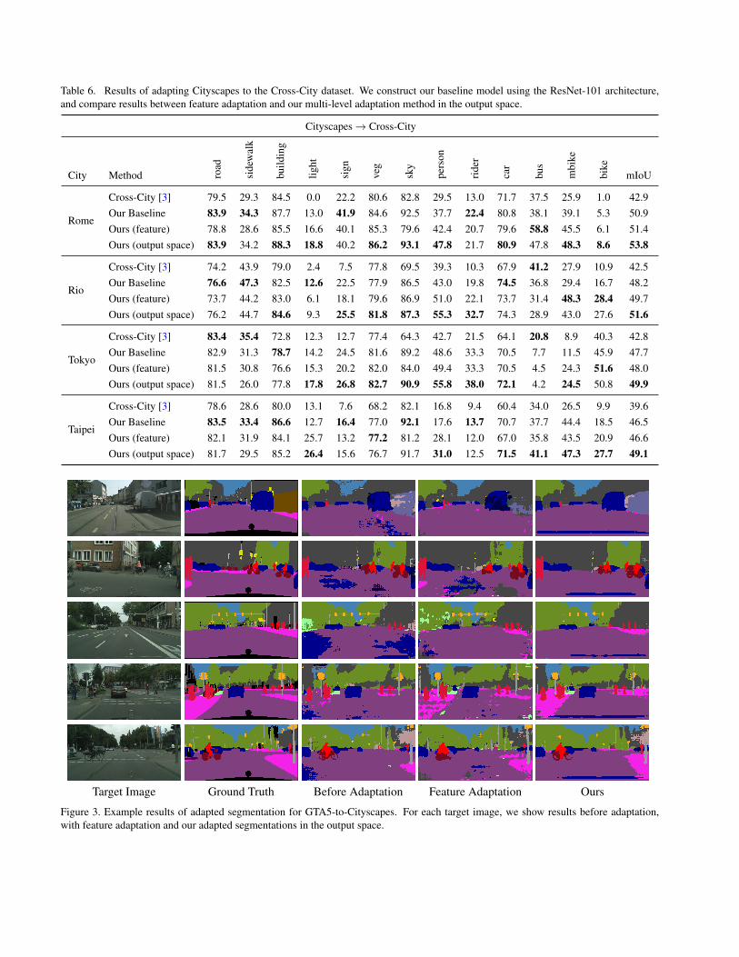
Table 6. Results of adapting Cityscapes to the Cross-City dataset. We construct our baseline model using the ResNet-101 architecture,and compare results between feature adaptation and our multi-level adaptation method in the output space.

Cityscapes → Cross-City

City Method road

side

wal

k

build

ing

light

sign

veg

sky

pers

on

ride

r

car

bus

mbi

ke

bike

mIoU

Rome

Cross-City [3] 79.5 29.3 84.5 0.0 22.2 80.6 82.8 29.5 13.0 71.7 37.5 25.9 1.0 42.9Our Baseline 83.9 34.3 87.7 13.0 41.9 84.6 92.5 37.7 22.4 80.8 38.1 39.1 5.3 50.9Ours (feature) 78.8 28.6 85.5 16.6 40.1 85.3 79.6 42.4 20.7 79.6 58.8 45.5 6.1 51.4Ours (output space) 83.9 34.2 88.3 18.8 40.2 86.2 93.1 47.8 21.7 80.9 47.8 48.3 8.6 53.8

Rio


Tokyo


Taipei


Target Image Ground Truth Before Adaptation Feature Adaptation Ours

Figure 3. Example results of adapted segmentation for GTA5-to-Cityscapes. For each target image, we show results before adaptation,with feature adaptation and our adapted segmentations in the output space.

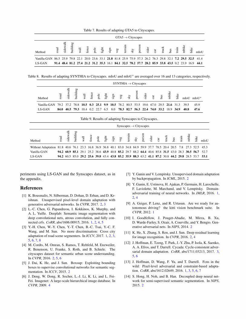
Table 7. Results of adapting GTA5 to Cityscapes.

GTA5→ Cityscapes

Method road

side

wal

k

build

ing

wal

l

fenc

e

pole

light

sign

veg

terr

ain

sky

pers

on

ride

r

car

truc

k

bus

trai

n

mbi

ke

bike

mIoU

Vanilla-GAN 86.5 25.9 79.8 22.1 20.0 23.6 33.1 21.8 81.8 25.9 75.9 57.3 26.2 76.3 29.8 32.1 7.2 29.5 32.5 41.4LS-GAN 91.4 48.4 81.2 27.4 21.2 31.2 35.3 16.1 84.1 32.5 78.2 57.7 28.2 85.9 33.8 43.5 0.2 23.9 16.9 44.1

Table 8. Results of adapting SYNTHIA to Cityscapes. mIoU and mIoU∗ are averaged over 16 and 13 categories, respectively.

SYNTHIA→ Cityscapes

Method road

side

wal

k

build

ing

wal

l

fenc

e

pole

light

sign

veg

sky

pers

on

ride

r

car

bus

mbi

ke

bike

mIoU mIoU∗

Vanilla-GAN 79.2 37.2 78.8 10.5 0.3 25.1 9.9 10.5 78.2 80.5 53.5 19.6 67.0 29.5 21.6 31.3 39.5 45.9LS-GAN 84.0 40.5 79.3 10.4 0.2 22.7 6.5 8.0 78.3 82.7 56.3 22.4 74.0 33.2 18.9 34.9 40.8 47.6

Table 9. Results of adapting Synscapes to Cityscapes.

Synscapes→ Cityscapes

Method road

side

wal

k

build

ing

wal

l

fenc

e

pole

light

sign

veg

terr

ain

sky

pers

on

ride

r

car

truc

k

bus

trai

n

mbi

ke

bike

mIoU

Without Adaptation 81.8 40.6 76.1 23.3 16.8 36.9 36.8 40.1 83.0 34.8 84.9 59.9 37.7 78.5 20.4 20.5 7.8 27.3 52.5 45.3Vanilla-GAN 94.2 60.9 85.1 29.1 25.2 38.6 43.9 40.8 85.2 29.7 88.2 64.4 40.6 85.8 31.5 43.0 28.3 30.5 56.7 52.7LS-GAN 94.2 60.5 85.0 29.2 25.6 39.8 43.4 43.8 85.2 35.9 88.3 63.2 41.1 87.2 30.8 44.2 29.8 28.5 53.7 53.1

periments using LS-GAN and the Synscapes dataset, as inthe appendix.

References[1] K. Bousmalis, N. Silberman, D. Dohan, D. Erhan, and D. Kr-

ishnan. Unsupervised pixel-level domain adaptation withgenerative adversarial networks. In CVPR, 2017. 2, 3

[2] L.-C. Chen, G. Papandreou, I. Kokkinos, K. Murphy, andA. L. Yuille. Deeplab: Semantic image segmentation withdeep convolutional nets, atrous convolution, and fully con-nected crfs. CoRR, abs/1606.00915, 2016. 1, 2, 4, 5

[3] Y.-H. Chen, W.-Y. Chen, Y.-T. Chen, B.-C. Tsai, Y.-C. F.Wang, and M. Sun. No more discrimination: Cross cityadaptation of road scene segmenters. In ICCV, 2017. 1, 2, 3,5, 6, 7, 8

[4] M. Cordts, M. Omran, S. Ramos, T. Rehfeld, M. Enzweiler,R. Benenson, U. Franke, S. Roth, and B. Schiele. Thecityscapes dataset for semantic urban scene understanding.In CVPR, 2016. 2, 5, 6

[5] J. Dai, K. He, and J. Sun. Boxsup: Exploiting boundingboxes to supervise convolutional networks for semantic seg-mentation. In ICCV, 2015. 2

[6] J. Deng, W. Dong, R. Socher, L.-J. Li, K. Li, and L. Fei-Fei. Imagenet: A large-scale hierarchical image database. InCVPR, 2009. 4

[7] Y. Ganin and V. Lempitsky. Unsupervised domain adaptationby backpropagation. In ICML, 2015. 2

[8] Y. Ganin, E. Ustinova, H. Ajakan, P. Germain, H. Larochelle,F. Laviolette, M. Marchand, and V. Lempitsky. Domain-adversarial training of neural networks. In JMLR, 2016. 1,2, 4

[9] A. Geiger, P. Lenz, and R. Urtasun. Are we ready for au-tonomous driving? the kitti vision benchmark suite. InCVPR, 2012. 1

[10] I. Goodfellow, J. Pouget-Abadie, M. Mirza, B. Xu,D. Warde-Farley, S. Ozair, A. Courville, and Y. Bengio. Gen-erative adversarial nets. In NIPS, 2014. 2

[11] K. He, X. Zhang, S. Ren, and J. Sun. Deep residual learningfor image recognition. In CVPR, 2016. 2, 4

[12] J. Hoffman, E. Tzeng, T. Park, J.-Y. Zhu, P. Isola, K. Saenko,A. A. Efros, and T. Darrell. Cycada: Cycle-consistent adver-sarial domain adaptation. CoRR, abs/1711.03213, 2017. 3,5, 6

[13] J. Hoffman, D. Wang, F. Yu, and T. Darrell. Fcns in thewild: Pixel-level adversarial and constraint-based adapta-tion. CoRR, abs/1612.02649, 2016. 1, 3, 5, 6, 7

[14] S. Hong, H. Noh, and B. Han. Decoupled deep neural net-work for semi-supervised semantic segmentation. In NIPS,2015. 2

[15] W.-C. Hung, Y.-H. Tsai, X. Shen, Z. Lin, K. Sunkavalli,X. Lu, and M.-H. Yang. Scene parsing with global contextembedding. In ICCV, 2017. 2

[16] S. Ioffe and C. Szegedy. Batch normalization: Acceleratingdeep network training by reducing internal covariate shift. InICML, 2015. 4

[17] A. Khoreva, R. Benenson, J. Hosang, M. Hein, andB. Schiele. Simple does it: Weakly supervised instance andsemantic segmentation. In CVPR, 2017. 2

[18] D. P. Kingma and J. Ba. Adam: A method for stochasticoptimization. In ICLR, 2015. 5

[19] A. Krizhevsky, I. Sutskever, and G. E. Hinton. Imagenetclassification with deep convolutional neural networks. InNIPS, 2012. 2

[20] C. Lee, S. Xie, P. W. Gallagher, Z. Zhang, and Z. Tu. Deeply-supervised nets. In AISTATS, 2015. 4

[21] G. Lin, C. Shen, A. van dan Hengel, and I. Reid. Efficientpiecewise training of deep structured models for semanticsegmentation. In CVPR, 2016. 1

[22] M.-Y. Liu and O. Tuzel. Coupled generative adversarial net-works. In NIPS, 2016. 2

[23] Z. Liu, X. Li, P. Luo, C. C. Loy, and X. Tang. Semantic im-age segmentation via deep parsing network. In ICCV, 2015.1

[24] J. Long, E. Shelhamer, and T. Darrell. Fully convolutionalnetworks for semantic segmentation. In CVPR, 2015. 1, 2, 6

[25] M. Long, Y. Cao, J. Wang, and M. Jordan. Learning transfer-able features with deep adaptation networks. In ICML, 2015.1, 2, 4

[26] M. Long, H. Zhu, J. Wang, and M. I. Jordan. Unsuperviseddomain adaptation with residual transfer networks. In NIPS,2016. 2

[27] A. L. Maas, A. Y. Hannun, and A. Y. Ng. Rectifier nonlin-earities improve neural network acoustic models. In ICML,2013. 4

[28] X. Mao, Q. Li, H. Xie, R. Y. Lau, Z. Wang, and S. Paul Smol-ley. Least squares generative adversarial networks. In ICCV,2017. 10

[29] G. Papandreou, L.-C. Chen, K. Murphy, and A. L. Yuille.Weakly-and semi-supervised learning of a dcnn for semanticimage segmentation. In ICCV, 2015. 2

[30] D. Pathak, P. Krahenbuhl, and T. Darrell. Constrained con-volutional neural networks for weakly supervised segmenta-tion. In ICCV, 2015. 2, 3

[31] A. Radford, L. Metz, and S. Chintala. Unsupervised repre-sentation learning with deep convolutional generative adver-sarial networks. In ICLR, 2016. 2, 4

[32] S. R. Richter, V. Vineet, S. Roth, and V. Koltun. Playing fordata: Ground truth from computer games. In ECCV, 2016.2, 5

[33] G. Ros, L. Sellart, J. Materzynska, D. Vazquez, andA. Lopez. The SYNTHIA Dataset: A large collection ofsynthetic images for semantic segmentation of urban scenes.In CVPR, 2016. 2, 5, 6

[34] K. Simonyan and A. Zisserman. Very deep convolutionalnetworks for large-scale image recognition. In ICLR, 2015.2

[35] K. Sohn, S. Liu, G. Zhong, X. Yu, M.-H. Yang, and M. Chan-draker. Unsupervised domain adaptation for face recognitionin unlabeled videos. In ICCV, 2017. 2

[36] Y.-H. Tsai, X. Shen, Z. Lin, K. Sunkavalli, X. Lu, and M.-H.Yang. Deep image harmonization. In CVPR, 2017. 1

[37] E. Tzeng, J. Hoffman, T. Darrell, and K. Saenko. Simultane-ous deep transfer across domains and tasks. In ICCV, 2015.2

[38] E. Tzeng, J. Hoffman, K. Saenko, and T. Darrell. Adversarialdiscriminative domain adaptation. In CVPR, 2017. 2

[39] M. Wrenninge and J. Unger. Synscapes: A photoreal-istic synthetic dataset for street scene parsing. CoRR,abs/1810.08705, 2018. 10

[40] F. Yu and V. Koltun. Multi-scale context aggregation by di-lated convolutions. In ICLR, 2016. 1, 2, 4, 6

[41] Y. Zhang, P. David, and B. Gong. Curriculum domain adap-tation for semantic segmentation of urban scenes. In ICCV,2017. 5, 6, 7

[42] H. Zhao, J. Shi, X. Qi, X. Wang, and J. Jia. Pyramid sceneparsing network. In CVPR, 2017. 1, 2, 4

[43] S. Zheng, S. Jayasumana, B. Romera-Paredes, V. Vineet,Z. Su, D. Du, C. Huang, and P. Torr. Conditional randomfields as recurrent neural networks. In ICCV, 2015. 1

[44] J.-Y. Zhu, T. Park, P. Isola, and A. A. Efros. Unpaired image-to-image translation using cycle-consistent adversarial net-works. ICCV, 2017. 3

A. Least Squares ObjectiveTo analyze the impact of different type of GANs in our

framework, we adopt the least-squares loss function in [28]that claims to generate higher-quality results and performmore stably during GAN training. The loss for discrimina-tor training, similar to (2), can be written as:

LLSd (P ) =

∑h,w

z(D(P )(h,w,1) − 1

)2(7)

+(1− z)(D(P )(h,w,0)

)2,

where z = 0 if the sample is drawn from the target domain,and z = 1 for the sample from the source domain. Similarto (4), the adversarial loss can be written as:

LLSadv(It) =

∑h,w

(D(Pt)

(h,w,1) − 1)2. (8)

We use the single-level adaptation network and the ResNet-101 backbone as in the main paper, and all the other detailsare the same. Results on Cityscapes using GTA5 and SYN-THIA as the source domain are presented in Table 7 andTable 8, respectively. We compare the performance of thevanilla GAN (as in the main paper) and the least-squares(LS) GAN. Both tables show that using the LS-GAN objec-tive achieves a higher mean IoU.

B. SynscapesThe Synscapes dataset [39] is a photorealistic synthetic

dataset for street scene parsing. It consists of 25, 000 RGBimages at 1440× 720 resolution. The ground truth annota-tion adopts the Cityscapes convention that contains 19 cat-egories. To adapt from Synscapes to Cityscapes, we use theentire Synsacpes dataset as the source domain. In Table 9,we show results without adaptation, with vanilla GAN, andLS-GAN, using the single-level adaptation network and theResNet-101 backbone.

Since the domain gap between Cityscapes and Synscapesis smaller than the case using either GTA5 or SYNTHIAas the source domain, the performance without adaptationalready achieves a mean IoU of 45.3%. By further usingoutput space adaptation, the vanilla and LS GAN objectivesimprove the results and perform competitively.

learning to adapt structured output space for semantic ... · learning to adapt structured output...

Documents