learning stable multilevel dictionaries for … · learning stable multilevel dictionaries for...

LEARNING STABLE MULTILEVEL DICTIONARIES FOR SPARSE REPRESENTATIONS 1

Learning Stable Multilevel Dictionaries forSparse Representations

Jayaraman J. Thiagarajan, Karthikeyan Natesan Ramamurthy and Andreas SpaniasE-mail: jjayaram,knatesan,[email protected].

Abstract—Sparse representations using learned dictionariesare being increasingly used with success in several data processingand machine learning applications. The availability of abundanttraining data necessitates the development of efficient, robustand provably good dictionary learning algorithms. Algorith-mic stability and generalization are desirable characteristicsfor dictionary learning algorithms that aim to build globaldictionaries which can efficiently model any test data similarto the training samples. In this paper, we propose an algorithmto learn dictionaries for sparse representations from large scaledata, and prove that the proposed learning algorithm is stableand generalizable asymptotically. The algorithm employs a 1-D subspace clustering procedure, the K-hyperline clustering, inorder to learn a hierarchical dictionary with multiple levels. Wealso propose an information-theoretic scheme to estimate thenumber of atoms needed in each level of learning and developan ensemble approach to learn robust dictionaries. Using theproposed dictionaries, the sparse code for novel test data canbe computed using a low-complexity pursuit procedure. Wedemonstrate the stability and generalization characteristics ofthe proposed algorithm using simulations. We also evaluate theutility of the multilevel dictionaries in compressed recovery andsubspace learning applications.

I. INTRODUCTION

A. Dictionary Learning for Sparse Representations

SEVERAL types of naturally occurring data have most oftheir energy concentrated in a small number of features

when represented using an linear model. In particular, it hasbeen shown that the statistical structure of naturally occurringsignals and images allows for their efficient representation as asparse linear combination of elementary features [1]. A finitecollection of normalized features is referred to as a dictionary.The linear model used for general sparse coding is given by

y = Ψa + n, (1)

where y ∈ RM is the data vector and Ψ = [ψ1ψ2 . . .ψK ] ∈RM×K is the dictionary. Each column of the dictionary,referred to as an atom, is a representative pattern normalizedto unit `2 norm. a ∈ RK is the sparse coefficient vector and nis a noise vector whose elements are independent realizationsfrom the Gaussian distribution N (0, σ2).

The sparse coding problem is usually solved as

a = argmina‖a‖0 subj. to ‖y −Ψa‖22 ≤ ε, (2)

where ‖.‖0 indicates the `0 sparsity measure which counts thenumber of non-zero elements, ‖.‖2 denotes the `2 norm and ε

The authors are with the SenSIP Center, School of Electrical, Computerand Energy Engineering, Arizona State University, Tempe, AZ, 85287.

is the error goal for the representation. The `1 norm, denotedby ‖.‖1, can be used instead of `0 measure to convexify (2).A variety of methods can be found in the literature to obtainsparse representations efficiently [2]–[5]. The sparse codingmodel has been successfully used for inverse problems inimages [6], and also in machine learning applications suchas classification, clustering, and subspace learning to name afew [7]–[16].

The dictionary Ψ used in (2) can be obtained from pre-defined bases, designed from a union of orthonormal bases[17], or structured as an overcomplete set of individual vectorsoptimized to the data [18]. A wide range of batch and onlinedictionary learning algorithms have been proposed in the liter-ature [19]–[27], some of which are tailored for specific tasks.The conditions under which a dictionary can be identifiedfrom the training data using an `1 minimization approach arederived in [28]. The joint optimization problem for dictionarylearning and sparse coding can be expressed as [6]

minΨ,A‖Y −ΨA‖2F subj. to ‖ai‖0 ≤ S, ∀i, ‖ψj‖2 = 1,∀j,

(3)where Y = [y1y2 . . .yT ] is a matrix of T training vectors,A = [a1a2 . . .aT ] is the coefficient matrix, S is the sparsityof the coefficient vector and ‖.‖F denotes the Frobenius norm.

B. Multilevel Learning

In this paper, we propose a hierarchical multilevel dictionarylearning algorithm that is implicitly regularized to aid in sparseapproximation of data. The proposed multilevel dictionary(MLD) learning algorithm is geared towards obtaining globaldictionaries for the entire probability space of the data, whichare provably stable, and generalizable to novel test data. Inaddition, our algorithm involves simple schemes for learningand representation: a 1-D subspace clustering algorithm (K-hyperline clustering [29]) is used to infer atoms in eachlevel, and 1−sparse representations are obtained in each levelusing a pursuit scheme that employs just correlate-and-maxoperations. In summary, the algorithm creates a sub-dictionaryfor each level and obtains a residual which is used as thetraining data for the next level, and this process is continueduntil a pre-defined stopping criterion is reached.

The primary utility of sparse models with learned dictionar-ies in data processing and machine learning applications stemsfrom the fact that the dictionary atoms serve as predictivefeatures, capable of providing a good representation for someaspect of the test data. From the viewpoint of statistical

arX

iv:1

303.

0448

v2 [

cs.C

V]

25

Sep

2013


learning theory [30], a good predictive model is one thatis stable and generalizable, and MLD learning satisfies boththese properties. To the best of our knowledge, there is noother dictionary learning method which has been proven tosatisfy these properties. Generalization ensures that the learneddictionary can successfully represent test data drawn fromthe same probability space as the training data, and stabilityguarantees that it is possible to reliably learn such a dictionaryfrom an arbitrary training set. In other words, the asymp-totic stability and generalization of MLD provides theoreticaljustification for the uniformly good performance of globalmultilevel dictionaries. We can minimize the risk of overfittingfurther by choosing a proper model order. We propose amethod based on the minimum description length (MDL)principle [31] to choose the optimal model order, which inour case corresponds to the number of dictionary elements ineach level. Recently, other approaches have been proposed tochoose the best order for a given sparse model using MDL[27], so that the generalization error is minimized. However,the difference in our case is that, in addition to optimizing themodel order for a given training set using MDL, we provethat any dictionary learned using MLD is generalizable andstable. Since both generalization and stability are asymptoticproperties, we also propose a robust variant of our MLDalgorithm using randomized ensemble methods, to obtain animproved performance with test data. Note that our goal is notto obtain dictionaries optimized for a specific task [24], but topropose a general predictive sparse modeling framework thatcan be suitably adapted for any task.

The dictionary atoms in MLD are structurally regularized,and therefore the hierarchy in representation is imposed im-plicitly for the novel test data, leading to improved recoveryin ill-posed and noise-corrupted problems. Considering dic-tionary learning with image patches as an example, in MLDthe predominant atoms in the first few levels (see Figure 1)always contribute the highest energy to the representation. Fornatural image data, it is known that the patches are comprisedof geometric patterns or stochastic textures or a combinationof both [32]. Since the geometric patterns usually are ofhigher energy when compared to stochastic textures in images,MLD learns the geometric patterns in the first few levels andstochastic textures in the last few levels, thereby adhering tothe natural hierarchy in image data. The hierarchical multistagevector quantization (MVQ) [33] is related to MLD learning.The important difference, however, is that dictionaries obtainedfor sparse representations must assume that the data lies in aunion-of-subspaces, and the MVQ does not incorporate thisassumption. Note that multilevel learning is also different fromthe work in [34], where multiple sub-dictionaries are designedand one of them is chosen for representing a group of patches.

C. Stability and Generalization in Learning

A learning algorithm is a map from the space of trainingexamples to the hypothesis space of functional solutions. Inclustering, the learned function is completely characterized bythe cluster centers. Stability of a clustering algorithm impliesthat the cluster centroids learned by the algorithm are not

significantly different when different sets of i.i.d. samplesfrom the same probability space are used for training [35].When there is a unique minimizer to the clustering objectivewith respect to the underlying data distribution, stability ofa clustering algorithm is guaranteed [36] and this analysishas been extended to characterize the stability of K-meansclustering in terms of the number of minimizers [37]. In[38], the stability properties of the K-hyperline clusteringalgorithm have been analyzed and they have been shown tobe similar to those of K-means clustering. Note that all thestability characterizations depend only on the underlying datadistribution and the number of clusters, and not on the actualtraining data itself. Generalization implies that the averageempirical training error becomes asymptotically close to theexpected error with respect to the probability space of data. In[39], the generalization bound for sparse coding in terms of thenumber of samples T , also referred to as sample complexity,is derived and in [40] the bound is improved by assuminga class of dictionaries that are nearly orthogonal. Clusteringalgorithms such as the K-means and the K-hyperline can beobtained by constraining the desired sparsity in (3) to be 1.Since the stability characteristics of clustering algorithms arewell understood, employing similar tools to analyze a generaldictionary learning framework such as MLD can be beneficial.

D. ContributionsIn this paper, we propose the MLD learning algorithm to

design global representative dictionaries for image patches.We show that, for a sufficient number of levels, the proposedalgorithm converges, and also demonstrate that a multileveldictionary with a sufficient number of atoms per level exhibitsenergy hierarchy (Section III-B). Furthermore, in order toestimate the number of atoms in each level of MLD, weprovide an information-theoretic approach based on the MDLprinciple (Section III-C). In order to compute sparse codesfor test data using the proposed dictionary, we develop thesimple Multilevel Pursuit (MulP) procedure and quantify itscomputational complexity (Section III-D). We also propose amethod to obtain robust dictionaries with limited training datausing ensemble methods (Section III-E). Some preliminaryalgorithmic details and results obtained using MLD have beenreported in [41].

Using the fact that the K-hyperline clustering algorithm isstable, we perform stability analysis of the MLD algorithm.For any two sets of i.i.d. training samples from the sameprobability space, as the number of training samples T →∞,we show that the dictionaries learned become close to eachother asymptotically. When there is a unique minimizer tothe objective in each level of learning, this holds true evenif the training sets are completely disjoint. However, whenthere are multiple minimizers for the objective in at least onelevel, we prove that the learned dictionaries are asymptoticallyclose when the difference between their corresponding trainingsets is o(

√T ). Instability of the algorithm when the difference

between two training sets is Ω(√T ), is also shown for the

case of multiple minimizers (Section IV-C). Furthermore, weprove the asymptotic generalization of the learning algorithm(Section IV-D).


In addition to demonstrating the stability and the general-ization behavior of MLD learning with image data (SectionsV-A and V-B), we evaluate its performance in compressedrecovery of images (Section V-C). Due to its theoreticalguarantees, the proposed MLD effectively recovers novel testimages from severe degradation (random projection). Inter-estingly, the proposed greedy pursuit with robust multileveldictionaries results in improved recovery performance whencompared to `1 minimization with online dictionaries, partic-ularly at reduced number of measurements and in presence ofnoise. Furthermore, we perform subspace learning with graphsconstructed using sparse codes from MLD and evaluate itsperformance in classification (Section V-D). We show thatthe proposed approach outperforms subspace learning withneighborhood graphs as well as graphs based on sparse codesfrom conventional dictionaries.

II. BACKGROUND

In this section, we describe the K-hyperline clustering, a 1-Dsubspace clustering procedure proposed in [29], which forms abuilding block of the proposed dictionary learning algorithm.Furthermore, we briefly discuss the results for stability analysisof K-means and K-hyperline algorithms reported in [35] and[38] respectively. The ideas described in this section will beused in Section IV to study the stability characteristics of theproposed dictionary learning procedure.

A. K-hyperline Clustering AlgorithmThe K-hyperline clustering algorithm is an iterative proce-

dure that performs a least squares fit of K 1-D linear subspacesto the training data [29]. Note that the K-hyperline clustering isa special case of general subspace clustering methods proposedin [42], [43], when the subspaces are 1−dimensional andconstrained to pass through the origin. In contrast with K-means, K-hyperline clustering allows each data sample to havean arbitrary coefficient value corresponding to the centroid ofthe cluster it belongs to. Furthermore, the cluster centroidsare normalized to unit `2 norm. Given the set of T datasamples Y = yiTi=1 and the number of clusters K, K-hyperline clustering proceeds in two stages after initialization:the cluster assignment and the cluster centroid update. Inthe cluster assignment stage, training vector yi is assignedto a cluster j based on the minimum distortion criteria,H(yi) = argminj d(yi,ψj), where the distortion measure is

d(y,ψ) = ‖y −ψ(yTψ)‖22. (4)

In the cluster centroid update stage, we perform singularvalue decomposition (SVD) of Yj = [yi]i∈Cj , where Cj =i|H(yi) = j contains indices of training vectors assignedto the cluster j. The cluster centroid is updated as the leftsingular vector corresponding to the largest singular value ofthe decomposition. This can also be computed using a lineariterative procedure. At iteration t+ 1, the jth cluster centroidis given by

ψ(t+1)j = YjY

Tj ψ

(t)j /‖YjY

Tj ψ

(t)j ‖2. (5)

Usually a few iterations are sufficient to obtain the centroidswith good accuracy.

B. Stability Analysis of Clustering Algorithms

Analyzing the stability of unsupervised clustering algo-rithms can be valuable in terms of understanding their behaviorwith respect to perturbations in the training set. These algo-rithms extract the underlying structure in the training data andthe quality of clustering is determined by an accompanyingcost function. As a result, any clustering algorithm can beposed as an Empirical Risk Minimization (ERM) procedure,by defining a hypothesis class of loss functions to evaluatethe possible cluster configurations and to measure their quality[44]. For example, K-hyperline clustering can be posed as anERM problem over the distortion function class

GK =

gΨ(y) = d(y,ψj), j = argmax

l∈1,··· ,K|yTψl|

. (6)

The class GK is constructed with functions gΨ correspondingto all possible combinations of K unit length vectors from theRM space for the set Ψ. Let us define the probability space forthe data in RM as (Y,Σ, P ), where Y is the sample space andΣ is a sigma-algebra on Y , i.e., the collection of subsets of Yover which the probability measure P is defined. The trainingsamples, yiTi=1, are i.i.d. realizations from this space.

Ideally, we are interested in computing the cluster centroidsΨ that minimize the expected distortion E[gΨ] with respectto the probability measure P . However, the underlying distri-bution of the data samples is not known and hence we resortto minimizing the average empirical distortion with respect tothe training samples yiTi=1 as

gΨ = argming∈GK

1

T

T∑i=1

gΨ(yi). (7)

When the empirical averages of the distortion functions in GKuniformly converge to the expected values over all probabilitymeasures P ,

limT→∞

supP

P

(sup

gΨ∈GK

∣∣∣∣∣E[gΨ]− 1

T

T∑i=1

gΨ(yi)

∣∣∣∣∣ > δ

)= 0,

(8)for any δ > 0, we refer to the class GK as uniform Glivenko-Cantelli (uGC). In addition, if the class also satisfies a versionof the central limit theorem, it is defined as uniform Donsker[44]. In order to determine if GK is uniform Donsker, wehave to verify if the covering number of GK with respectto the supremum norm, N∞(γ,GK), grows polynomially inthe dimensions M [35]. Here, γ denotes the maximum L∞distance between an arbitrary distortion function in GK , andthe function that covers it. For K-hyperline clustering, thecovering number is upper bounded by [38, Lemma 2.1]

N∞(γ,GK) ≤(

8R3K + γ

γ

)MK

, (9)

where we assume that the data lies in an M -dimensional `2ball of radius R centered at the origin. Therefore, GK belongsto the uniform Donsker class.

Stability implies that the algorithm should produce clustercentroids that are not significantly different when differenti.i.d. sets from the same probability space are used for training


[35]–[37]. Stability is characterized based on the number ofminimizers to the clustering objective with respect to theunderlying data distribution. A minimizer corresponds to afunction gΨ ∈ GK with the minimum expectation E[gΨ].Stability analysis of K-means clustering has been reported in[35], [37]. Though the geometry of K-hyperline clustering isdifferent from that of K-means, the stability characteristics ofthe two algorithms have been found to be similar [38].

Given two sets of cluster centroids Ψ = ψ1, . . . ,ψKand Λ = λ1, . . . ,λK learned from training sets of T i.i.d.samples each realized from the same probability space, let usdefine the L1(P ) distance between the clusterings as

‖gΨ − gΛ‖L1(P ) =

∫|gΨ(y)− gΛ(y)|dP (y). (10)

When T →∞, and GK is uniform Donsker, stability in termsof the distortion functions is expressed as

‖gΨ − gΛ‖L1(P )P−→ 0, (11)

where P−→ denotes convergence in probability. This holds trueeven for Ψ and Λ learned from completely disjoint trainingsets, when there is a unique minimizer to the clusteringobjective. When there are multiple minimizers, (11) holdstrue with respect to a change in o(

√T ) samples between

two training sets and fails to hold with respect to a changein Ω(

√T ) samples [38]. The distance between the cluster

centroids themselves is defined as [35]

∆(Ψ,Λ) = max1≤j≤K

min1≤l≤K

[(d(ψj ,λl))

1/2 + (d(ψl,λj))1/2].

(12)

Lemma 2.1 ( [38]): If the L1(P ) distance between the dis-tortion functions for the clusterings Ψ and Λ is bounded as‖gΨ − gΛ‖L1(P ) < µ, for some µ > 0, and dP (y)/dy > C,for some C > 0, then ∆(Ψ,Λ) ≤ 2 sin(ρ) where

ρ ≤ 2 sin−1

1

r

(µ

CC,M

) 1M+1

. (13)

Here the training data is assumed to lie outside an M -dimensional `2 ball of radius r centered at the origin, andthe constant CC,M depends only on C and M .When the clustering algorithm is stable according to (11),for admissible values of r, Lemma 2.1 shows that the clustercentroids become arbitrarily close to each other.

III. MULTILEVEL DICTIONARY LEARNING

In this section, we develop the multilevel dictionary learningalgorithm, whose algorithmic stability and generalizability willbe proved in Section IV. Furthermore, we propose strategiesto estimate the number of atoms in each level and make thelearning process robust for improved generalization. We alsopresent a simple pursuit scheme to compute representationsfor novel test data using the MLD.

TABLE IALGORITHM FOR BUILDING A MULTILEVEL DICTIONARY.

InputY = [yi]

Ti=1, M × T matrix of training vectors.

L, maximum number of levels of the dictionary.Kl, number of dictionary elements in level l, l = 1, 2, ..., L.ε, error goal of the representation.

OutputΨl, adapted sub-dictionary for level l.

AlgorithmInitialize: l = 1 and R0 = Y.Λ0 = i | ‖r0,i‖22 > ε, 1 ≤ i ≤ T, index of training vectors withsquared norm greater than error goal.R0 = [r0,i]i∈Λ0

.

while Λl−1 6= ∅ and l ≤ LInitialize:

Al, coefficient matrix, size Kl ×M , all zeros.Rl, residual matrix for level l, size M × T , all zeros.Ψl, Al = KLC(Rl−1,Kl).Rtl = Rl−1 −ΨlAl.

rl,i = rtl,j where i = Λl−1(j), ∀j = 1, ..., |Λl−1|.al,i = al,j where i = Λl−1(j), ∀j = 1, ..., |Λl−1|.Λl = i | ‖rl,i‖22 > ε, 1 ≤ i ≤ T.Rl =

[rl,i

]i∈Λl

.l← l + 1.

end

A. Algorithm

We denote the MLD as Ψ = [Ψ1Ψ2...ΨL], and thecoefficient matrix as A = [AT

1 AT2 ...A

TL]T . Here, Ψl is the

sub-dictionary and Al is the coefficient matrix for level l. Theapproximation in level l is expressed as

Rl−1 = ΨlAl + Rl, for l = 1, ..., L, (14)

where Rl−1, Rl are the residuals for the levels l − 1 andl respectively and R0 = Y, the matrix of training imagepatches. This implies that the residual matrix in level l − 1serves as the training data for level l. Note that the sparsityof the representation in each level is fixed at 1. Hence, theoverall approximation for all levels is

Y =

L∑l=1

ΨlAl + RL. (15)

MLD learning can be interpreted as a block-based dictio-nary learning problem with unit sparsity per block, wherethe sub-dictionary in each block can allow only a 1-sparserepresentation and each block corresponds to a level. Thesub-dictionary for level l, Ψl, is the set of cluster centroidslearned from the training matrix for that level, Rl−1, usingK-hyperline clustering. MLD learning can be formally statedas an optimization problem that proceeds from the first leveluntil the stopping criteria is reached. For level l, we solve

argminΨl,Al

‖Rl−1 −ΨlAl‖2F subject to ‖al,i‖0 ≤ 1,

for i = 1, ..., T, (16)

along with the constraint that the columns of Ψl have unit`2 norm, where al,i is the ith column of Al and T is the


number of columns in Al. We adopt the notation Ψl,Al =KLC(Rl−1,Kl) to denote the problem in (16) where Kl isthe number of atoms in Ψl. The stopping criteria is providedeither by imposing a limit on the residual representation erroror the maximum number of levels (L). Note that the totalnumber of levels is the same as the maximum number ofnon-zero coefficients (sparsity) of the representation. The errorconstraint can be stated as, ‖rl,i‖22 ≤ ε,∀i = 1, ..., T , whererl,i is the ith column in Rl, and ε is the error goal.

Table I lists the MLD learning algorithm with a fixed L. Weuse the notation Λl(j) to denote the jth element of the set Λl.The set Λl contains the indices of the residual vectors of level lwhose norm is greater than the error goal. The residual vectorsindexed by Λl are stacked in the matrix, Rl, which in turnserves as the training matrix for the next level, l+ 1. In MLDlearning, for a given level l, the residual rl,i is orthogonal tothe representation Ψlal,i. This implies that

‖rl−1,i‖22 = ‖Ψlal,i‖22 + ‖rl,i‖22. (17)

Combining this with the fact that yi =∑Ll=1 Ψlal,i + rL,i,

al,i is 1−sparse, and the columns of Ψl are of unit `2 norm,we obtain the relation

‖yi‖22 =

L∑l=1

‖al,i‖22 + ‖rL,i‖22. (18)

Equation (18) states that the energy of any training vector isequal to the sum of squares of its coefficients and the energyof its residual. From (17), we also have that,

‖Rl−1‖2F = ‖ΨlAl‖2F + ‖Rl‖2F . (19)

The training vectors for the first level of the algorithm, r0,i liein the ambient RM space and the residuals, r1,i, lie in a finiteunion of RM−1 subspaces. This is because, for each dictionaryatom in the first level, its residual lies in an M − 1 dimensionalspace orthogonal to it. In the second level, the dictionary atomscan possibly lie anywhere in RM , and hence the residualscan lie in a finite union of RM−1 and RM−2 dimensionalsubspaces. Hence, we can generalize that the dictionary atomsfor all levels lie in RM , whereas the training vectors of levell ≥ 2, lie in finite unions of RM−1, . . . ,RM−l+1 dimensionalsubspaces of the RM space.

B. Convergence

The convergence of MLD learning and the energy hierarchyin the representation obtained using an MLD can be shown byproviding two guarantees. The first guarantee is that for a fixednumber of atoms per level, the algorithm will converge to therequired error within a sufficient number of levels. This isbecause the K-hyperline clustering makes the residual energyof the representation smaller than the energy of the trainingmatrix at each level (i.e.) ‖Rl‖2F < ‖Rl−1‖2F . This followsfrom (19) and the fact that ‖ΨlAl‖2F > 0.

The second guarantee is that for a sufficient number ofatoms per level, the representation energy in level l will beless than the representation energy in level l − 1. To showthis, we first state that for a sufficient number of dictionary

atoms per level, ‖ΨlAl‖2F > ‖Rl‖2F . This means that forevery l

‖Rl‖2F < ‖ΨlAl‖2F < ‖Rl−1‖2F , (20)

because of (19). This implies that ‖ΨlAl‖2F <‖Ψl−1Al−1‖2F , i.e., the energy of the representation ineach level reduces progressively from l = 1 to l = L, therebyexhibiting energy hierarchy.

C. Estimating Number of Atoms in Each Level

The number of atoms in each level of an MLD can beoptimally estimated using an information theoretic criteriasuch as minimum description length (MDL) [31]. The broadidea is that the model order, which is the number of dictionaryatoms here, is chosen to minimize the total description lengthneeded for representing the model and the data given themodel. The codelength for encoding the data Y given themodel Θ is given as the negative log likelihood − log p(Y|Θ).The description length for the model is the number of bitsneeded to code the model parameters.

In order to estimate the number of atoms in each levelusing the MDL principle, we need to make some assumptionson the residual obtained in each level. Our first assumptionwill be that the a fraction α of the total energy in eachlevel El will be represented at that level and the remainingenergy (1 − α)El will be the residual energy. The residualand the representation energy sum up to the total energyin each level because, the residual in any level of MLD isorthogonal to the representation in that level. Therefore, atany level l, the represented energy will be α(1−α)l−1E andthe residual energy will be (1 − α)lE, where E is the totalenergy of training data at the first level. For simplicity, we alsoassume that the residual at each level follows the zero-meanmultinormal distribution N (0, σ2

l IM ). Combining these twoassumptions, the variance is estimated as σ2

l = 1MT (1−α)lE.

The total MDL score, which is an indicator of theinformation-theoretic complexity, is the sum of the negativelog likelihood and the number of bits needed to encodethe model. Encoding the model includes encoding the non-zero coefficients, their location, and the dictionary elementsthemselves. The MDL score for level l with the data Rl−1,dictionary Ψl ∈ RM×Kl , and the coefficient matrix Al is

MDL(Rl−1|Ψl,Al,Kl) =1

2σ2l

T∑i=1

‖rl−1,i −Ψlal,i‖22

+1

2T log(MT ) + T log(TKl) +

1

2KlM log(MT ). (21)

Here, the first term in the sum represents the data descriptionlength, which is also the negative log-likelihood of the dataafter ignoring the constant term. The second term is thenumber of bits needed to code the T non-zero coefficientsas reals where each coefficient is coded using 0.5 log(MT )bits [45]. The third term denotes the bits needed to codetheir locations which are integers between 1 and TKl, andthe fourth term represents the total bits needed to code all thedictionary elements as reals. The optimal model order Kl isthe number of dictionary atoms that results in the least MDL


Fig. 1. The top 4 levels and the last level of the MLD dictionary wherethe number of atoms are estimated using the MDL procedure. It comprisesof geometric patterns in the first few levels and stochastic textures in the lastlevel. Since each level has a different number of atoms, each sub-dictionaryis padded with zero vectors, which appear as black patches.

score. In practice, we test a finite number of model orders andpick the one which results in the least score. As an example,we train a dictionary using 5000 grayscale patches of size 8×8from the BSDS dataset [46]. We preprocess the patches byvectorizing them and subtracting the mean of each vectorizedpatch from its elements. We perform MLD learning andestimate the estimate the optimal number of dictionary atomsin each level using α = 0.25, for a maximum of 16 levels. Forthe sub-dictionary in each level, the number of atoms werevaried between 10 and 50, and one that provided the leastMDL score was chosen as optimal. The first few levels and thelast level of the MLD obtained using such procedure is shownin Figure 1. The minimum MDL score obtained in each levelis shown in 2. From these two figures, clearly, the information-theoretic complexity of the sub-dictionaries increase with thenumber of levels, and the atoms themselves progress frombeing simple geometric structures to stochastic textures.

D. Sparse Approximation using an MLD

In order to compute sparse codes for novel test data using amultilevel dictionary, we propose to perform reconstruction us-ing a Multilevel Pursuit (MulP) procedure which evaluates a 1-sparse representation for each level using the dictionary atomsfrom that level. Therefore, the coefficient vector for the ith datasample rl,i in level l is obtained using a simple correlate-and-max operation, whereby we compute the correlations ΨT

l rl,iand pick the coefficient value and index corresponding to themaximum absolute correlation. The computational complexityof a correlate-and-max operation is of order MKl and hencethe complexity of obtaining the full representation using Llevels is of order MK, where K =

∑Li=1Kl is the total

number of atoms in the dictionary. Whereas, the complexityof obtaining an L sparse representation on the full dictionaryusing Orthogonal Matching Pursuit is of order LMK.

E. Robust Multilevel Dictionaries

Although MLD learning is a simple procedure capable ofhandling large scale data with useful asymptotic generalizationproperties as described in Section (IV-D), the procedure canbe made robust and its generalization performance can beimproved using randomization schemes. The Robust MLD(RMLD) learning scheme, which is closely related to Rvotes[47] - a supervised ensemble learning method, improves thegeneralization performance of MLD as evidenced by Figure8. The Rvotes scheme randomly samples the training set tocreate D sets of TD samples each, where TD T . Thefinal prediction is obtained by averaging the predictions from

Fig. 2. The minimum MDL score of each level. The information-theoreticcomplexity of the sub-dictionaries increase with the number of levels.

the multiple hypotheses learned from the training sets. Forlearning level l in RMLD, we draw D subsets of randomlychosen training samples, Y(d)

l Dd=1 from the original trainingset Yl of size T , allowing for overlap across the subsets. Notethat here, Yl = Rl−1. The superscript here denotes the indexof the subset. For each subset Y

(d)l of size TD T , we

learn a sub-dictionary Ψ(d)l with Kl atoms using K-hyperline

clustering. For each training sample in Yl, we compute1−sparse representations using all the D sub-dictionaries,and denote the set of coefficient matrices as A(d)

l Dd=1. Theapproximation for the ith training sample in level l, yl,i, iscomputed as the average of approximations using all D sub-dictionaries, 1

D

∑d Ψ

(d)l a

(d)l,i . The ensemble approximations

for all training samples in the level can be used to computethe set of residuals, and this process is repeated for a desirednumber of levels, to obtain an RMLD.

Reconstruction of test data with an RMLD is performedby extending the multilevel pursuit. We obtain D approxi-mations for each data sample at a given level, average theapproximations, compute the residual and repeat this for thesubsequent levels. Note that this can also be implemented asmultiple correlate-and-max operations per data sample perlevel. Clearly, the computational complexity for obtaining asparse representation using the RMLD is of order DMK,where K =

∑Li=1Kl.

IV. STABILITY AND GENERALIZATION

In this section, the behavior of the proposed dictionarylearning algorithm is considered from the viewpoint of algo-rithmic stability: the behavior of the algorithm with respectto the perturbations in the training set. It will be shownthat the dictionary atoms learned by the algorithm from twodifferent training sets whose samples are realized from thesame probability space, become arbitrarily close to each other,as the number of training samples T → ∞. Since theproposed MLD learning is equivalent to learning K-hyperlinecluster centroids in multiple levels, the stability analysis of


K-hyperline clustering [38], briefly discussed in Section II-B,will be utilized in order to prove its stability. For each levelof learning, the cases of single and multiple minimizers tothe clustering objective will be considered. Proving that thelearning algorithm is stable will show that the global dictio-naries learned from the data depend only on the probabilityspace to which the training samples belong and not on theactual samples themselves, as T →∞. We also show that theMLD learning generalizes asymptotically, i.e., the differencebetween expected error and average empirical error in trainingapproaches zero, as T → ∞. Therefore, the expected errorfor novel test data, drawn from the same distribution as thetraining data, will approach the average empirical trainingerror.

The stability analysis of the MLD algorithm will be per-formed by considering two different dictionaries Ψ and Λ withL levels each. Each level consists of Kl dictionary atoms andthe sub-dictionaries in each level are indicated by Ψl and Λl

respectively. Sub-dictionaries Ψl and Λl are the cluster centerslearned using K-hyperline clustering on the training data forlevel l. The steps involved in proving the overall stability ofthe algorithm are: (a) showing that each level of the algorithmis stable in terms of L1(P ) distance between the distortionfunctions, defined in (10), as the number of training samplesT →∞ (Section IV-A), (b) proving that stability in terms ofL1(P ) distances indicates closeness of the centers of the twoclusterings (Section IV-B), in terms of the metric defined in(12), and (c) showing that level-wise stability leads to overallstability of the dictionary learning algorithm (Section IV-C).

A. Level-wise Stability

Let us define a probability space (Yl,Σl, Pl) where Yl isthe data that lies in RM , and Pl is the probability measure.The training samples for the sub-dictionaries Ψl and Λl aretwo different sets of T i.i.d. realizations from the probabilityspace. We also assume that the `2 norm of the training samplesis bounded from above and below (i.e.), 0 < r ≤ ‖y‖2 ≤ R <∞. Note that, in a general case, the data will lie in RM forthe first level of dictionary learning and in a finite union oflower-dimensional subspaces of RM for the subsequent levels.In both cases, the following argument on stability will hold.This is because when the training data lies in a union of lowerdimensional subspaces of RM , we can assume it to be stilllying in RM , but assign the probabilities outside the union ofsubspaces to be zero.

The distortion function class for the clusterings, definedsimilar to (6), is uniform Donsker because the covering num-ber with respect to the supremum norm grows polynomially,according to (9). When a unique minimizer exists for theclustering objective, the distortion functions corresponding tothe different clusterings Ψl and Λl become arbitrarily close,‖gΨl

− gΛl‖L1(Pl)

P−→ 0, even for completely disjoint trainingsets, as T →∞. However, in the case of multiple minimizers,‖gΨl

− gΛl‖L1(Pl)

P−→ 0 holds only with respect to a changeof o(

√T ) training samples between the two clusterings, and

fails to hold for a change of Ω(√T ) samples [35], [38].

B. Distance between Cluster Centers for a Stable Clustering

For each cluster center in the clustering Ψl, we pick theclosest cluster center from Λl, in terms of the distortionmeasure (4), and form pairs. Let us indicate the jth pair ofcluster centers by ψl,j and λl,j . Let us define τ disjoint setsAiτi=1, in which the training data for the clusterings exist,such that Pl(∪τi=1Ai) = 1. By defining such disjoint sets, wecan formalize the notion of training data lying in a union ofsubspaces of RM . The intuitive fact that the cluster centersof two clusterings are close to each other, given that theirdistortion functions are close, is proved in the lemma below.

Lemma 4.1: Consider two sub-dictionaries (clusterings) Ψl

and Λl with Kl atoms each obtained using the T trainingsamples that exist in the τ disjoint sets Aiτi=1 in the RMspace, with 0 < r ≤ ‖y‖2 ≤ R < ∞, and dPl(y)/dy >C in each of the sets. When the distortion functions becomearbitrarily close to each other, ‖gΨl

− gΛl‖L1(Pl)

P−→ 0 asT → ∞, the smallest angle between the subspaces spannedby the cluster centers becomes arbitrarily close to zero, i.e.,

∠(ψl,j ,λl,j)P−→ 0, ,∀j ∈ 1, . . . ,Kl. (22)

Proof: Denote the smallest angle between the subspacesrepresented by ψl,j and λl,j as ∠(ψl,j , λl,j) = ρl,j anddefine a region S(ψl,j , ρl,j/2) = y|∠(ψl,j ,y) ≤ ρl,j/2, 0 <r ≤ ‖y‖2 ≤ R < ∞. If y ∈ S(ψl,j , ρl,j/2), thenyT (I−ψl,jψ

Tl,j)y ≤ yT (I−λl,jλTl,j)y. An illustration of this

setup for a 2-D case is given in Figure 3. In this figure, thearc q1q2 is of radius r and represents the minimum value of‖y‖2. By definition, the L1(Pl) distance between the distortionfunctions of the clusterings for data that exists in the disjointsets Aiτi=1 is

‖gΨl − gΛl‖L1(Pl) =

τ∑i=1

∫Ai

|gΨl(y)− gΛl(y)|dPl(y). (23)

For any j and i with a non-empty Bl,i,j = S(ψl,j , ρl,j/2)∩Aiwe have,

‖gΨl − gΛl‖L1(Pl) ≥∫Bl,i,j

|gΨl(y)− gΛl(y)|dPl(y), (24)

=

∫Bl,i,j

[yT(I− λl,jλTl,j

)y −

K∑k=1

yT(I−ψl,kψ

Tl,k

)y

I(y closest to ψl,k

) ]dPl(y), (25)

≥∫Bl,i,j

[yT(I− λl,jλTl,j

)y − yT

(I−ψl,jψ

Tl,j

)y]dPl(y),

(26)

≥ C

∫Bl,i,j

[(yTψl,j

)2

−(yTλl,j

)2]dy. (27)

We have gΛl(y) = yT

(I− λl,jλTl,j

)y in (25), since λl,j is

the closest cluster center to the data in S(ψl,j , ρl,j/2)∩Ai interms of the distortion measure (4). Note that I is the indicatorfunction and (27) follows from (26) because dPl(y)/dy > C.Since by assumption, ‖gΨl

− gΛl‖L1(Pl)

P−→ 0, from (27), wehave (

yTψl,j)2 − (yTλl,j)2 P−→ 0, (28)


Fig. 3. Illustration for showing the stability of cluster centroids from thestability of distortion function.

because the integrand in (27) is a continuous non-negativefunction in the region of integration.

Denoting the smallest angles between y and the subspacesspanned by ψl,j and λl,j to be θψl,j

and θλl,jrespectively,

from (28), we have ‖y‖22(cos2 θψl,j− cos2 θλl,j

)P−→ 0, for

all y. By definition of the region Bl,i,j , we have θψl,j≤

θλl,j. Since ‖y‖2 is bounded away from zero and infinity, if

(cos2 θψl,j− cos2 θλl,j

)P−→ 0 holds for all y ∈ Bl,i,j , then

we have ∠(ψl,j ,λl,j)P−→ 0. This is true for all cluster center

pairs as we have shown this for an arbitrary i and j.

C. Stability of the MLD Algorithm

The stability of the MLD algorithm as a whole, is proved inTheorem 4.3 from its level-wise stability by using an inductionargument. The proof will depend on the following lemmawhich shows that the residuals from two stable clusteringsbelong to the same probability space.

Lemma 4.2: When the training vectors for the sub-dictionaries (clusterings) Ψl and Λl are obtained from theprobability space (Yl,Σl, Pl), and the cluster center pairsbecome arbitrarily close to each other as T → ∞, the resid-ual vectors from both the clusterings belong to an identicalprobability space (Yl+1,Σl+1, Pl+1).

Proof: For the jth cluster center pair ψl,j , λl,j , defineΨl,j and Λl,j as the projection matrices for their respectiveorthogonal complement subspaces ψ⊥l,j and λ⊥l,j . Define thesets Dψl,j

= y ∈ Ψl,j(β + dβ) + ψl,jα and Dλl,j=

y ∈ Λl,j(β + dβ) + λl,jα, where −∞ < α < ∞, βis an arbitrary fixed vector, not orthogonal to both ψl,j andλl,j , and dβ is a differential element. The residual vector setfor the cluster ψl,j , when y ∈ Dψl,j

is given by, rψl,j∈

Ψl,jy|y ∈ Dψl,j, or equivalently rψl,j

∈ Ψl,j(β + dβ).Similarly for the cluster λl,j , we have rλl,j

∈ Λl,j(β+dβ).For a 2-D case, Figure 4 shows the 1-D subspace ψl,j , itsorthogonal complement ψ⊥l,j , the set Dψl,j

and the residualset Ψl,j(β + dβ).

In terms of probabilities, we also have that Pl(y ∈ Dψl,j) =

Pl+1(rψl,j∈ Ψl,j(β + dβ)), because the residual set

Fig. 4. The residual set Ψl,j(β+ dβ), for the 1-D subspace ψl,j , lyingin its orthogonal complement subspace ψ⊥l,j .

Ψl,j(β + dβ) is obtained by a linear transformation ofDψl,j

. Here Pl and Pl+1 are probability measures definedon the training data for levels l and l + 1 respectively.Similarly, Pl(y ∈ Dλl,j

) = Pl+1(rλl,j∈ Λl,j(β + dβ)).

When T → ∞, the cluster center pairs become arbitrarilyclose to each other, i.e., ∠(ψl,j ,λl,j)

P−→ 0, by assumption.Therefore, the symmetric difference between the sets Dψl,j

and Dλl,japproaches the null set, which implies that Pl(y ∈

Dψl,j)− Pl(y ∈ Dλl,j

)→ 0. This implies,

Pl+1(rψl,j∈ Ψl,j(β + dβ))−Pl+1(rλl,j

∈ Λl,j(β + dβ))→ 0, (29)

for an arbitrary β and dβ, as T → ∞. This means that theresiduals of ψl,j and λl,j belong to a unique but identicalprobability space. Since we proved this for an arbitrary l and j,we can say that the residuals of clusterings Ψl and Λl belongto an identical probability space given by (Yl+1,Σl+1, Pl+1).

Theorem 4.3: Given that the training vectors for the firstlevel are generated from the probability space (Y1,Σ1, P1),and the norms of training vectors for each level are boundedas 0 < r ≤ ‖y‖2 ≤ R < ∞, the MLD learning algorithm isstable as a whole.

Proof: The level-wise stability of MLD was shown inSection IV-A, for two cases: (a) when a unique minimizerexists for the distortion function and (b) when a uniqueminimizer does not exist. Lemma 4.1 proved that the stabilityin terms of closeness of distortion functions implied stabilityin terms of learned cluster centers. For showing the level-wisestability, we assumed that the training vectors in level l forclusterings Ψl and Λl belonged to the same probability space.However, when learning the dictionary, this is true only for thefirst level, as we supply the algorithm with training vectorsfrom the probability space (Y1,Σ1, P1).

We note that the training vectors for level l+1 are residualsof the clusterings Ψl and Λl. Lemma 4.2 showed that theresiduals of level l for both the clusterings belong to anidentical probability space (Yl+1,Σl+1, Pl+1), given that thetraining vectors of level l are realizations from the probability


Fig. 5. Demonstration of the stability behavior of the proposed MLDlearning algorithm. The minimum Frobenius norm between difference of twodictionaries with respect to permutation of their columns and signs is shown.The second dictionary is obtained by replacing different number of samplesin the training set, used for training the original dictionary, with new datasamples.

space (Yl,Σl, Pl) and T → ∞. By induction, this alongwith the fact that the training vectors for level 1 belong tothe same probability space (Y1,Σ1, P1), shows that all thetraining vectors of both the dictionaries for any level l indeedbelong to a probability space (Yl,Σl, Pl) corresponding tothat level. Hence all the levels of the dictionary learning arestable and the MLD learning is stable as a whole. Similar toK-hyperline clustering, if there are multiple minimizers in atleast one level, the algorithm is stable only with respect to achange of o(

√T ) training samples between the two clusterings

and failts to hold for a change of Ω(√T ) samples.

D. Generalization Analysis

Since our learning algorithm consists of multiple levels, andcannot be expressed as an ERM on a whole, the algorithm canbe said to generalize asymptotically if the sum of empiricalerrors for all levels converge to the sum of expected errors, asT →∞. This can be expressed as∣∣∣∣∣ 1

T

L∑l=1

T∑i=1

gΨl(yl,i)−

L∑l=1

EPl[gΨl

]

∣∣∣∣∣ P−→ 0, (30)

where the training samples for level l given by yl,iTi=1 areobtained from the probability space (Yl,Σl, Pl). When (30)holds and the learning algorithm generalizes, it can be seenthat the expected error for test data which is drawn from thesame probability space as that of the training data, is close tothe average empirical error. Therefore, when the cluster centersfor each level are obtained by minimizing the empirical error,the expected test error will also be small.

In order to show that (30) holds, we use the fact thateach level of MLD learning is obtained using K-hyperlineclustering. Hence, from (8), the average empirical distortionin each level converges to the expected distortion as T →∞,∣∣∣∣∣ 1

T

T∑i=1

gΨl(yl,i)− EPl

[gΨl]

∣∣∣∣∣ P−→ 0. (31)

Fig. 6. Choosing the number of rounds (R) in RMLD learning. In thisdemonstration, RMLD design was carried out using 100, 000 samples andwe observed that beyond 10, both the train MSE and the test MSE do notchange significantly.

The validity of the condition in (30) follows directly from thetriangle inequality,∣∣∣∣∣ 1

T

L∑l=1

T∑i=1

gΨl(yl,i)−

L∑l=1

EPl[gΨl

]

∣∣∣∣∣≤

L∑l=1

∣∣∣∣∣ 1

T

T∑i=1

gΨl(yl,i)− EPl

[gΨl]

∣∣∣∣∣ . (32)

If the MulP coding scheme is used for test data, andthe training and test data for level 1 are obtained fromthe probability space (Y1,Σ1, P1), the probability space forboth training and test data in level l will be (Yl,Σl, Pl).This is because, both the MulP coding scheme and MLDlearning associate the data to a dictionary atom using themaximum absolute correlation measure and create a residualthat is orthogonal to the atom chosen in a level. Hence, theassumption that training and test data are drawn from the sameprobability space in all levels hold and the expected test errorwill be similar to the average empirical training error.

V. SIMULATION RESULTS

In this section, we present experiments to demonstrate thestability and generalization characteristics of a multilevel dic-tionary, and evaluate its use in compressed recovery of imagesand subspace learning. Both stability and generalization arecrucial for building effective global dictionaries that can modelpatterns in any novel test image. Although it is not possibleto demonstrate the asymptotic behavior experimentally, westudy the changes in the behavior of the learning algorithmwith increase in the number of samples used for training.Compressed recovery is a highly relevant application for globaldictionaries, since it is not possible to infer dictionaries withgood reconstructive power directly from the low-dimensionalrandom measurements of image patches. It is typical to employboth `1 minimization and greedy pursuit methods for recover-ing images from their compressed measurements. Though `1minimization incurs higher computational complexity, it oftenprovides improved recovery performance when compared togreedy approaches. Hence, it is important to compare itsrecovery performance to that of the MLD that uses a simple


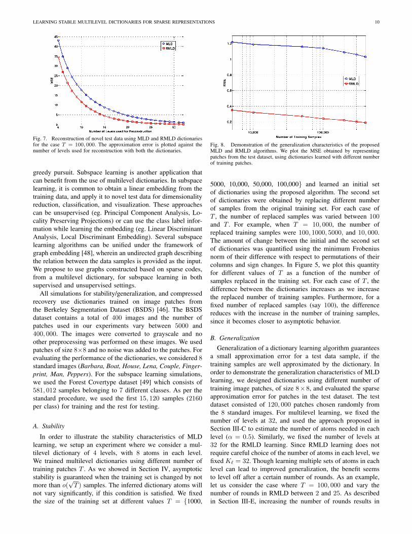
Fig. 7. Reconstruction of novel test data using MLD and RMLD dictionariesfor the case T = 100, 000. The approximation error is plotted against thenumber of levels used for reconstruction with both the dictionaries.

greedy pursuit. Subspace learning is another application thatcan benefit from the use of multilevel dictionaries. In subspacelearning, it is common to obtain a linear embedding from thetraining data, and apply it to novel test data for dimensionalityreduction, classification, and visualization. These approachescan be unsupervised (eg. Principal Component Analysis, Lo-cality Preserving Projections) or can use the class label infor-mation while learning the embedding (eg. Linear DiscriminantAnalysis, Local Discriminant Embedding). Several subspacelearning algorithms can be unified under the framework ofgraph embedding [48], wherein an undirected graph describingthe relation between the data samples is provided as the input.We propose to use graphs constructed based on sparse codes,from a multilevel dictionary, for subspace learning in bothsupervised and unsupervised settings.

All simulations for stability/generalization, and compressedrecovery use dictionaries trained on image patches fromthe Berkeley Segmentation Dataset (BSDS) [46]. The BSDSdataset contains a total of 400 images and the number ofpatches used in our experiments vary between 5000 and400, 000. The images were converted to grayscale and noother preprocessing was performed on these images. We usedpatches of size 8×8 and no noise was added to the patches. Forevaluating the performance of the dictionaries, we considered 8standard images (Barbara, Boat, House, Lena, Couple, Finger-print, Man, Peppers). For the subspace learning simulations,we used the Forest Covertype dataset [49] which consists of581, 012 samples belonging to 7 different classes. As per thestandard procedure, we used the first 15, 120 samples (2160per class) for training and the rest for testing.

A. Stability

In order to illustrate the stability characteristics of MLDlearning, we setup an experiment where we consider a mul-tilevel dictionary of 4 levels, with 8 atoms in each level.We trained multilevel dictionaries using different number oftraining patches T . As we showed in Section IV, asymptoticstability is guaranteed when the training set is changed by notmore than o(

√T ) samples. The inferred dictionary atoms will

not vary significantly, if this condition is satisfied. We fixedthe size of the training set at different values T = 1000,

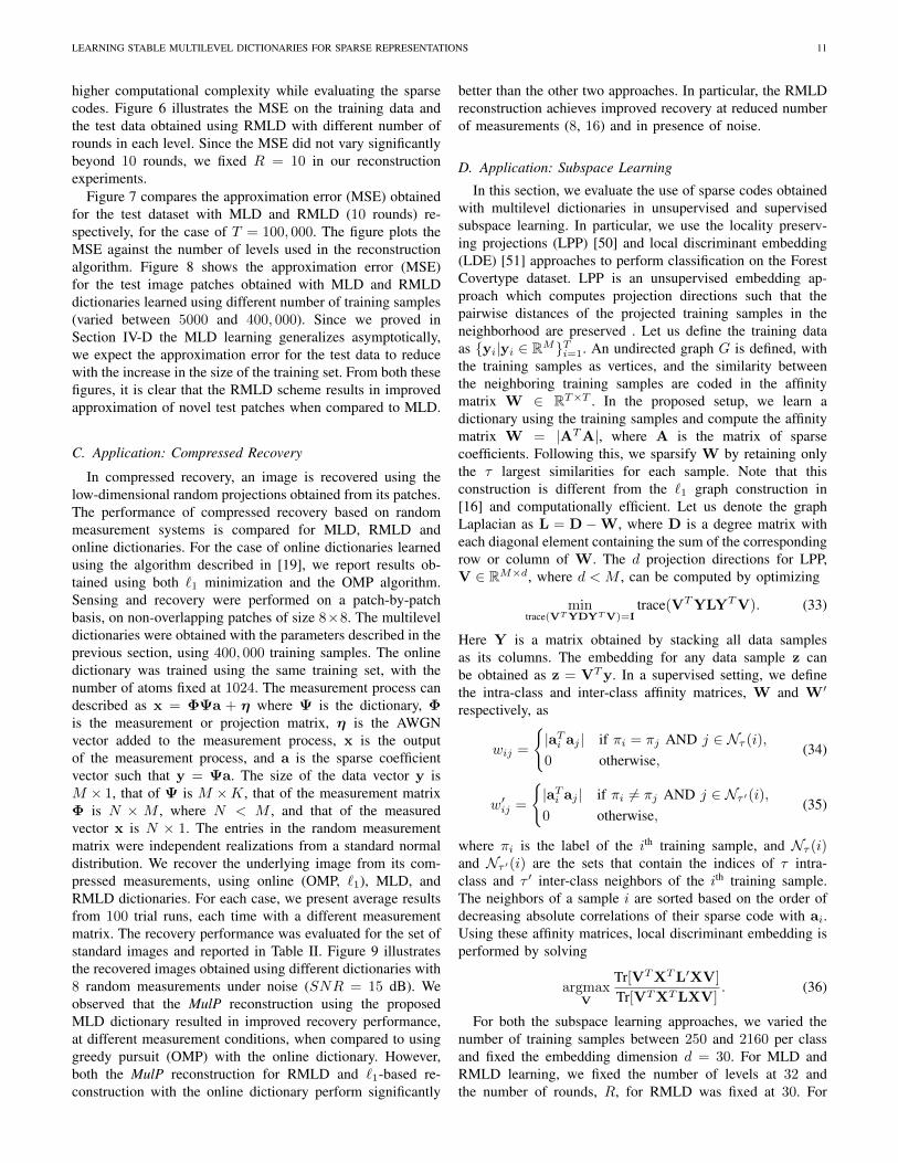
Fig. 8. Demonstration of the generalization characteristics of the proposedMLD and RMLD algorithms. We plot the MSE obtained by representingpatches from the test dataset, using dictionaries learned with different numberof training patches.

5000, 10,000, 50,000, 100,000 and learned an initial setof dictionaries using the proposed algorithm. The second setof dictionaries were obtained by replacing different numberof samples from the original training set. For each case ofT , the number of replaced samples was varied between 100and T . For example, when T = 10, 000, the number ofreplaced training samples were 100, 1000, 5000, and 10, 000.The amount of change between the initial and the second setof dictionaries was quantified using the minimum Frobeniusnorm of their difference with respect to permutations of theircolumns and sign changes. In Figure 5, we plot this quantityfor different values of T as a function of the number ofsamples replaced in the training set. For each case of T , thedifference between the dictionaries increases as we increasethe replaced number of training samples. Furthermore, for afixed number of replaced samples (say 100), the differencereduces with the increase in the number of training samples,since it becomes closer to asymptotic behavior.

B. Generalization

Generalization of a dictionary learning algorithm guaranteesa small approximation error for a test data sample, if thetraining samples are well approximated by the dictionary. Inorder to demonstrate the generalization characteristics of MLDlearning, we designed dictionaries using different number oftraining image patches, of size 8×8, and evaluated the sparseapproximation error for patches in the test dataset. The testdataset consisted of 120, 000 patches chosen randomly fromthe 8 standard images. For multilevel learning, we fixed thenumber of levels at 32, and used the approach proposed inSection III-C to estimate the number of atoms needed in eachlevel (α = 0.5). Similarly, we fixed the number of levels at32 for the RMLD learning. Since RMLD learning does notrequire careful choice of the number of atoms in each level, wefixed K` = 32. Though learning multiple sets of atoms in eachlevel can lead to improved generalization, the benefit seemsto level off after a certain number of rounds. As an example,let us consider the case where T = 100, 000 and vary thenumber of rounds in RMLD between 2 and 25. As describedin Section III-E, increasing the number of rounds results in


higher computational complexity while evaluating the sparsecodes. Figure 6 illustrates the MSE on the training data andthe test data obtained using RMLD with different number ofrounds in each level. Since the MSE did not vary significantlybeyond 10 rounds, we fixed R = 10 in our reconstructionexperiments.

Figure 7 compares the approximation error (MSE) obtainedfor the test dataset with MLD and RMLD (10 rounds) re-spectively, for the case of T = 100, 000. The figure plots theMSE against the number of levels used in the reconstructionalgorithm. Figure 8 shows the approximation error (MSE)for the test image patches obtained with MLD and RMLDdictionaries learned using different number of training samples(varied between 5000 and 400, 000). Since we proved inSection IV-D the MLD learning generalizes asymptotically,we expect the approximation error for the test data to reducewith the increase in the size of the training set. From both thesefigures, it is clear that the RMLD scheme results in improvedapproximation of novel test patches when compared to MLD.

C. Application: Compressed Recovery

In compressed recovery, an image is recovered using thelow-dimensional random projections obtained from its patches.The performance of compressed recovery based on randommeasurement systems is compared for MLD, RMLD andonline dictionaries. For the case of online dictionaries learnedusing the algorithm described in [19], we report results ob-tained using both `1 minimization and the OMP algorithm.Sensing and recovery were performed on a patch-by-patchbasis, on non-overlapping patches of size 8×8. The multileveldictionaries were obtained with the parameters described in theprevious section, using 400, 000 training samples. The onlinedictionary was trained using the same training set, with thenumber of atoms fixed at 1024. The measurement process candescribed as x = ΦΨa + η where Ψ is the dictionary, Φis the measurement or projection matrix, η is the AWGNvector added to the measurement process, x is the outputof the measurement process, and a is the sparse coefficientvector such that y = Ψa. The size of the data vector y isM × 1, that of Ψ is M ×K, that of the measurement matrixΦ is N × M , where N < M , and that of the measuredvector x is N × 1. The entries in the random measurementmatrix were independent realizations from a standard normaldistribution. We recover the underlying image from its com-pressed measurements, using online (OMP, `1), MLD, andRMLD dictionaries. For each case, we present average resultsfrom 100 trial runs, each time with a different measurementmatrix. The recovery performance was evaluated for the set ofstandard images and reported in Table II. Figure 9 illustratesthe recovered images obtained using different dictionaries with8 random measurements under noise (SNR = 15 dB). Weobserved that the MulP reconstruction using the proposedMLD dictionary resulted in improved recovery performance,at different measurement conditions, when compared to usinggreedy pursuit (OMP) with the online dictionary. However,both the MulP reconstruction for RMLD and `1-based re-construction with the online dictionary perform significantly

better than the other two approaches. In particular, the RMLDreconstruction achieves improved recovery at reduced numberof measurements (8, 16) and in presence of noise.

D. Application: Subspace Learning

In this section, we evaluate the use of sparse codes obtainedwith multilevel dictionaries in unsupervised and supervisedsubspace learning. In particular, we use the locality preserv-ing projections (LPP) [50] and local discriminant embedding(LDE) [51] approaches to perform classification on the ForestCovertype dataset. LPP is an unsupervised embedding ap-proach which computes projection directions such that thepairwise distances of the projected training samples in theneighborhood are preserved . Let us define the training dataas yi|yi ∈ RMTi=1. An undirected graph G is defined, withthe training samples as vertices, and the similarity betweenthe neighboring training samples are coded in the affinitymatrix W ∈ RT×T . In the proposed setup, we learn adictionary using the training samples and compute the affinitymatrix W = |ATA|, where A is the matrix of sparsecoefficients. Following this, we sparsify W by retaining onlythe τ largest similarities for each sample. Note that thisconstruction is different from the `1 graph construction in[16] and computationally efficient. Let us denote the graphLaplacian as L = D −W, where D is a degree matrix witheach diagonal element containing the sum of the correspondingrow or column of W. The d projection directions for LPP,V ∈ RM×d, where d < M , can be computed by optimizing

mintrace(VT YDYT V)=I

trace(VTYLYTV). (33)

Here Y is a matrix obtained by stacking all data samplesas its columns. The embedding for any data sample z canbe obtained as z = VTy. In a supervised setting, we definethe intra-class and inter-class affinity matrices, W and W′

respectively, as

wij =

|aTi aj | if πi = πj AND j ∈ Nτ (i),

0 otherwise,(34)

w′ij =

|aTi aj | if πi 6= πj AND j ∈ Nτ ′(i),

0 otherwise,(35)

where πi is the label of the ith training sample, and Nτ (i)and Nτ ′(i) are the sets that contain the indices of τ intra-class and τ ′ inter-class neighbors of the ith training sample.The neighbors of a sample i are sorted based on the order ofdecreasing absolute correlations of their sparse code with ai.Using these affinity matrices, local discriminant embedding isperformed by solving

argmaxV

Tr[VTXTL′XV]

Tr[VTXTLXV]. (36)

For both the subspace learning approaches, we varied thenumber of training samples between 250 and 2160 per classand fixed the embedding dimension d = 30. For MLD andRMLD learning, we fixed the number of levels at 32 andthe number of rounds, R, for RMLD was fixed at 30. For


TABLE IIPSNR (DB) OF THE IMAGES RECOVERED FROM COMPRESSED MEASUREMENTS OBTAINED USING GAUSSIAN RANDOM MEASUREMENT MATRICES.

RESULTS OBTAINED WITH THE ONLINE (OMP), ONLINE (`1), RMLD (MULP), AND MLD (MULP) ALGORITHMS ARE GIVEN IN CLOCKWISE ORDERBEGINNING FROM TOP LEFT CORNER. HIGHER PSNR FOR EACH CASE IS INDICATED IN BOLD FONT.

SNR (dB) # Measurements Boat House Lena Man Peppers

0

821.43 22.32 22.43 23.36 23.13 24.05 22.23 23.13 19.08 20.0121.60 22.43 22.86 23.76 23.52 24.39 22.43 23.28 19.55 20.43

1622.19 23.19 23.31 24.39 24.02 25.03 22.98 23.97 19.97 21.0522.67 23.60 24.18 25.15 24.76 25.75 23.51 24.46 20.96 21.95

3223.50 24.18 24.94 25.48 25.54 26.08 24.26 24.95 21.71 22.1424.18 25.15 25.94 27.03 26.46 27.54 25.02 26.02 22.87 23.90

15

822.77 23.65 23.95 24.97 24.61 25.60 23.58 24.46 20.61 21.6823.48 24.45 25.11 26.14 25.69 26.70 24.34 25.31 21.90 22.90

1623.94 26.33 25.36 28.65 26.03 28.92 24.74 27.08 22.28 25.4325.29 26.56 27.43 28.71 27.83 29.12 26.09 27.36 24.34 25.60

3226.33 30.19 28.16 33.59 28.55 33.17 26.48 30.64 25.21 29.7828.13 29.96 30.77 33.41 30.88 32.94 28.81 30.44 27.48 29.47

25

822.82 23.73 24.01 25.09 24.66 25.70 23.63 24.54 20.67 21.8323.62 24.56 25.27 26.30 25.85 26.83 24.47 25.42 22.05 23.04

1624.00 26.57 25.44 29.11 26.10 29.30 24.81 27.32 22.37 25.8725.55 26.84 27.80 29.23 28.15 29.48 26.35 27.63 24.68 25.99

3226.38 30.77 28.71 34.81 28.61 33.98 27.13 31.15 25.97 30.7428.72 30.45 31.67 34.57 31.63 33.67 29.37 30.87 28.28 30.54

(a) Online-OMP (24.73 dB) (b) Online-`1 (25.69 dB) (c) MLD-MulP (26.02 dB) (d) RMLD-MulP (27.41 dB)

Fig. 9. Compressed recovery of images from random measurements (N = 8, SNR of measurement process = 15dB) using the different dictionaries. Ineach case the PSNR of the recovered image is also shown.

comparison, we use learned iterative dictionaries of size 1024,using `1 minimization in the SPAMS toolbox [19] and theLagrangian dual method (SC-LD) [52] . Finally, classificationwas performed using a simple 1−nearest neighbor classifier.Table III and Table IV show the classification accuraciesobtained using the different dictionaries, for both the subspacelearning approaches. As it can be observed, graphs constructedwith the proposed multilevel dictionaries provide more dis-criminative embeddings compared to the other approaches.

VI. CONCLUSIONS

We presented a multilevel learning algorithm to designgeneralizable and stable global dictionaries for sparse rep-resentations. The proposed algorithm uses multiple levelsof 1−D subspace clustering to learn dictionaries. We alsoproposed a method to infer the number of atoms in each level,and provided an ensemble learning approach to create robust

dictionaries. We proved that the learning algorithm converges,exhibits energy hierarchy, and is also generalizable and stable.Finally, we demonstrated the superior performance of MLDin applications such as compressive sensing and subspacelearning. Future research could include providing an onlineframework for MLD that can work with streaming data, andalso developing hierarchical dictionaries that are optimized forrobust penalties on reconstruction error.

REFERENCES

[1] D. J. Field, “What is the goal of sensory coding?” Neural Comp., vol. 6,pp. 559–601, 1994.

[2] J. A. Tropp and S. J. Wright, “Computational methods for sparse solutionof linear inverse problems,” Proc. IEEE, vol. 98, no. 6, pp. 948–958,2010.

[3] S. S. Chen, D. L. Donoho, and M. A. Saunders, “Atomic decompositionby basis pursuit,” SIAM Review, vol. 43, no. 1, pp. 129–159, 2001.

[4] M. Elad et.al., “A wide-angle view at iterated shrinkage algorithms,” inSPIE, 2007.


TABLE IIIUNSUPERVISED SUBSPACE LEARNING - CLASSIFICATION ACCURACIES

WITH A 1-NN CLASSIFIER.

# Train Graph Construction ApproachPer Class LPP SC-LD SC-MLD SC-RMLD

250 57.11 57.5 58.2 58.9500 58.8 59.9 61.35 62.581000 66.33 67.6 68.94 69.911500 70.16 71.32 73.65 74.382160 74.39 75.8 78.26 78.84

TABLE IVSUPERVISED SUBSPACE LEARNING - CLASSIFICATION ACCURACIES WITH

A 1-NN CLASSIFIER.

# Train Graph Construction ApproachPer Class LDE SC-LD SC-MLD SC-RMLD

250 59.23 59.1 59.3 59.6500 60.4 60.8 61.9 62.71000 68.1 68.71 69.6 70.431500 72.9 73.5 74.41 75.092160 77.3 78.07 79.53 80.01

[5] B. Efron, T. Hastie, I. Johnstone, and R. Tibshirani, “Least angleregression,” The Annals of statistics, vol. 32, no. 2, pp. 407–499, 2004.

[6] M. Aharon, M. Elad, and A. Bruckstein, “K-SVD: An algorithm fordesigning overcomplete dictionaries for sparse representation,” IEEETSP, vol. 54, no. 11, pp. 4311–4322, November 2006.

[7] K. Huang and S. Aviyente, “Sparse representation for signal classifica-tion,” in NIPS, 2006.

[8] J. J. Thiagarajan, K. N. Ramamurthy, P. Knee, and A. Spanias, “Sparserepresentations for automatic target classification in SAR images,” inISCCSP, 2010.

[9] J. Wright et.al., “Robust face recognition via sparse representation,”IEEE TPAMI, vol. 31, no. 2, pp. 210–227, 2001.

[10] I. Ramirez, P. Sprechmann, and G. Sapiro, “Classification and clusteringvia dictionary learning with structured incoherence and shared features,”in IEEE CVPR, Jun. 2010, pp. 3501 –3508.

[11] J. Yang et.al., “Linear spatial pyramid matching using sparse coding forimage classification,” in IEEE CVPR, 2009.

[12] G. Yu, G. Sapiro, and S. Mallat, “Image modeling and enhancement viastructured sparse model selection,” in IEEE ICIP, Sep. 2010, pp. 1641–1644.

[13] Q. Zhang and B. Li, “Discriminative K-SVD for dictionary learning inface recognition,” in IEEE CVPR, 2010.

[14] Z. Jiang et.al., “Learning a discriminative dictionary for sparse codingvia label consistent K-SVD,” in IEEE CVPR, 2011.

[15] J. J. Thiagarajan, K. N. Ramamurthy, P. Sattigeri, and A. Spanias, “Su-pervised local sparse coding of sub-image features for image retrieval,”in IEEE ICIP, 2012.

[16] B. Cheng, J. Yang, S. Yan, Y. Fu, and T. S. Huang, “Learning with`1-graph for image analysis.” IEEE TIP, vol. 19, no. 4, pp. 858–66, apr2010.

[17] R. Gribonval and M. Nielsen, “Sparse representations in unions ofbases,” IEEE Trans. Inf. Theory, vol. 49, no. 12, pp. 3320–3325, 2003.

[18] M. S. Lewicki and T. J. Sejnowski, “Learning overcomplete representa-tions,” Neural Comp., vol. 12, no. 2, pp. 337–365, 2000.

[19] J. Mairal, F. Bach, J. Ponce, and G. Sapiro, “Online learning for matrixfactorization and sparse coding,” JMLR, vol. 11, no. 1, pp. 19–60, 2009.

[20] R. Jenatton, J. Mairal, G. Obozinski, and F. Bach, “Proximal methodsfor sparse hierarchical dictionary learning,” in ICML, J. Frankranz andT. Joachims, Eds. Omnipress, 2010, pp. 487–494.

[21] L. Bar and G. Sapiro, “Hierarchical dictionary learning for invariantclassification,” in IEEE ICASSP, March 2010, pp. 3578–3581.

[22] R. Rubinstein, A. Bruckstein, and M. Elad, “Dictionaries for sparserepresentation modeling,” Proc. IEEE, vol. 98, no. 6, pp. 1045–1057,2010.

[23] I. Tosic and P. Frossard, “Dictionary learning,” IEEE Sig. Proc. Mag.,vol. 28, no. 2, pp. 27–38, 2011.

[24] J. Mairal, F. Bach, and J. Ponce, “Task-driven dictionary learning,” IEEEPAMI, vol. 34, no. 4, pp. 791–804, 2012.

[25] Y. Zhou and K. Barner, “Locality constrained dictionary learning fornonlinear dimensionality reduction,” IEEE SP Letters, 2012.

[26] H. Wang, C. Yuan, W. Hu, and C. Sun, “Supervised class-specificdictionary learning for sparse modeling in action recognition,” Patt. Rec.,vol. 45, no. 11, pp. 3902–3911, 2012.

[27] I. Ramırez and G. Sapiro, “An MDL framework for sparse coding anddictionary learning,” IEEE TSP, vol. 60, no. 6, pp. 2913–2927, 2012.

[28] R. Gribonval and K. Schnass, “Dictionary Identification - Sparse Matrix-Factorisation via `1-Minimisation,” IEEE Trans. on Inf. Theory, vol. 56,no. 7, pp. 3523–3539, Jul. 2010.

[29] Z. He et.al., “K-hyperline clustering learning for sparse componentanalysis,” Sig. Proc., vol. 89, pp. 1011–1022, 2009.

[30] T. Poggio, R. Rifkin, S. Mukherjee, and P. Niyogi, “General conditionsfor predictivity in learning theory,” Nature, vol. 428, no. 6981, pp. 419–422, 2004.

[31] P. D. Grunwald, I. J. Myung, and M. A. Pitt, Advances in minimumdescription length: Theory and applications. MIT press, 2005.

[32] S. Zhu, K. Shi, and Z. Si, “Learning explicit and implicit visualmanifolds by information projection,” Patt. Rec. Letters, vol. 31, pp.667–685, 2010.

[33] A. Gersho and R. Gray, Vector Quantization and Signal Compression.Boston: Kluwer Academic Publishers, 1992.

[34] G. Yu, G. Sapiro, and S. Mallat, “Image modeling and enhancement viastructured sparse model selection,” in IEEE ICIP, 2010.

[35] A. Rakhlin and A. Caponnetto, “Stability of K-means clustering,” in Ad-vances in Neural Information Processing Systems, vol. 19. Cambridge,MA: MIT Press, 2007.

[36] S. Ben-David, U. von Luxburg, and D. Pal, “A sober look at clusteringstability,” Conference on Computational Learning Theory, pp. 5–19,2006.

[37] S. Ben-David, D. Pal, and H. U. Simon, “Stability of K-means clus-tering,” ser. Lecture Notes in Computer Science, vol. 4539. Springer,2007, pp. 20–34.

[38] J. J. Thiagarajan, K. N. Ramamurthy, and A. Spanias, “Optimality andstability of the K-hyperline clustering algorithm,” Patt. Rec. Letters,2010.

[39] A. Maurer and M. Pontil, “K-Dimensional Coding Schemes in HilbertSpaces,” IEEE Trans. on Inf. Theory, vol. 56, no. 11, pp. 5839–5846,2010.

[40] D. Vainsencher and A. M. Bruckstein, “The Sample Complexity ofDictionary Learning,” JMLR, vol. 12, pp. 3259–3281, 2011.

[41] J. J. Thiagarajan, K. N. Ramamurthy, and A. Spanias, “Multileveldictionary learning for sparse representation of images,” in IEEE DSPWorkshop, 2011.

[42] P. Agarwal and N. Mustafa, “K-means projective clustering,” in ACMSIGMOD-SIGACT-SIGART symposium on Principles of database sys-tems. ACM, 2004, pp. 155–165.

[43] P. Tseng, “Nearest q-flat to m points,” Journal of Optimization Theoryand Applications, vol. 105, no. 1, pp. 249–252, 2000.

[44] A. Caponnetto and A. Rakhlin, “Stability properties of empirical riskminimization over Donsker classes,” JMLR, vol. 7, pp. 2565–2583, 2006.

[45] N. Saito, “Simultaneous noise suppression and signal compression usinga library of orthonormal bases and the minimum description lengthcriterion,” Wavelets in Geophysics, vol. 4, pp. 299–324, 1994.

[46] “Berkeley segmentation dataset,” Available athttp://www.eecs.berkeley.edu/Research/Projects/CS/vision/grouping/segbench/.

[47] L. Breiman, “Pasting small votes for classification in large databasesand on-line,” Machine Learning, vol. 36, no. 1, pp. 85–103, 1999.

[48] S. Yan, D. Xu, B. Zhang, H.-J. Zhang, Q. Yang, and S. Lin, “Graphembedding and extensions: a general framework for dimensionalityreduction,” IEEE PAMI, vol. 29, no. 1, pp. 40–51, 2007.

[49] K. Bache and M. Lichman, “UCI machine learning repository,” 2013.[Online]. Available: http://archive.ics.uci.edu/ml

[50] X. He and P. Niyogi, “Locality preserving projections,” in NIPS, 2003.[51] H.-T. Chen, H.-W. Chang, and T.-L. Liu, “Local discriminant embedding

and its variants,” in IEEE CVPR, vol. 2, 2005, pp. 846–853.[52] H. Lee, A. Battle, R. Raina, and A. Ng, “Efficient sparse coding

algorithms,” in NIPS, 2006, pp. 801–808.

http://archive.ics.uci.edu/ml

learning stable multilevel dictionaries for … · learning stable multilevel dictionaries for...

Documents