Learning Spherical Convolutionfor Fast Features from 360° Imagery

Yu-Chuan Su Kristen GraumanThe University of Texas at Austin

Abstract

While 360° cameras offer tremendous new possibilities in vision, graphics, andaugmented reality, the spherical images they produce make core feature extrac-tion non-trivial. Convolutional neural networks (CNNs) trained on images fromperspective cameras yield “flat" filters, yet 360° images cannot be projected to asingle plane without significant distortion. A naive solution that repeatedly projectsthe viewing sphere to all tangent planes is accurate, but much too computationallyintensive for real problems. We propose to learn a spherical convolutional networkthat translates a planar CNN to process 360° imagery directly in its equirectan-gular projection. Our approach learns to reproduce the flat filter outputs on 360°data, sensitive to the varying distortion effects across the viewing sphere. The keybenefits are 1) efficient feature extraction for 360° images and video, and 2) theability to leverage powerful pre-trained networks researchers have carefully honed(together with massive labeled image training sets) for perspective images. Wevalidate our approach compared to several alternative methods in terms of both rawCNN output accuracy as well as applying a state-of-the-art “flat" object detectorto 360° data. Our method yields the most accurate results while saving orders ofmagnitude in computation versus the existing exact reprojection solution.

1 Introduction

Unlike a traditional perspective camera, which samples a limited field of view of the 3D sceneprojected onto a 2D plane, a 360° camera captures the entire viewing sphere surrounding its opticalcenter, providing a complete picture of the visual world—an omnidirectional field of view. As such,viewing 360° imagery provides a more immersive experience of the visual content compared totraditional media.

360° cameras are gaining popularity as part of the rising trend of virtual reality (VR) and augmentedreality (AR) technologies, and will also be increasingly influential for wearable cameras, autonomousmobile robots, and video-based security applications. Consumer level 360° cameras are now commonon the market, and media sharing sites such as Facebook and YouTube have enabled support for360° content. For consumers and artists, 360° cameras free the photographer from making real-timecomposition decisions. For VR/AR, 360° data is essential to content creation. As a result of this greatpotential, computer vision problems targeting 360° content are capturing the attention of both theresearch community and application developer.

Immediately, this raises the question: how to compute features from 360° images and videos?Arguably the most powerful tools in computer vision today are convolutional neural networks (CNN).CNNs are responsible for state-of-the-art results across a wide range of vision problems, includingimage recognition [17, 42], object detection [12, 30], image and video segmentation [16, 21, 28], andaction detection [10, 32]. Furthermore, significant research effort over the last five years (and reallydecades [27]) has led to well-honed CNN architectures that, when trained with massive labeled imagedatasets [8], produce “pre-trained" networks broadly useful as feature extractors for new problems.

31st Conference on Neural Information Processing Systems (NIPS 2017), Long Beach, CA, USA.

φ

θ

Input: 360◦ image

Strategy I φ

θ

EquirectangularProjection

· · ·Fully ConvolutionNp

Sample n

PerspectiveProjection

Strategy II

· · · · · ·Output

Np · · ·Np · · ·

Np

Figure 1: Two existing strategies for applying CNNs to 360° images. Top: The first strategy unwraps the360° input into a single planar image using a global projection (most commonly equirectangular projection),then applies the CNN on the distorted planar image. Bottom: The second strategy samples multiple tangentplanar projections to obtain multiple perspective images, to which the CNN is applied independently to obtainlocal results for the original 360° image. Strategy I is fast but inaccurate; Strategy II is accurate but slow. Theproposed approach learns to replicate flat filters on spherical imagery, offering both speed and accuracy.

Indeed such networks are widely adopted as off-the-shelf feature extractors for other algorithms andapplications (c.f., VGG [33], ResNet [17], and AlexNet [25] for images; C3D [36] for video).

However, thus far, powerful CNN features are awkward if not off limits in practice for 360° imagery.The problem is that the underlying projection models of current CNNs and 360° data are different.Both the existing CNN filters and the expensive training data that produced them are “flat", i.e., theproduct of perspective projection to a plane. In contrast, a 360° image is projected onto the unitsphere surrounding the camera’s optical center.

To address this discrepancy, there are two common, though flawed, approaches. In the first, thespherical image is projected to a planar one,1 then the CNN is applied to the resulting 2D image [19,26](see Fig. 1, top). However, any sphere-to-plane projection introduces distortion, making the resultingconvolutions inaccurate. In the second existing strategy, the 360° image is repeatedly projectedto tangent planes around the sphere, each of which is then fed to the CNN [34, 35, 38, 41] (Fig. 1,bottom). In the extreme of sampling every tangent plane, this solution is exact and therefore accurate.However, it suffers from very high computational cost. Not only does it incur the cost of renderingeach planar view, but also it prevents amortization of convolutions: the intermediate representationcannot be shared across perspective images because they are projected to different planes.

We propose a learning-based solution that, unlike the existing strategies, sacrifices neither accuracynor efficiency. The main idea is to learn a CNN that processes a 360° image in its equirectangularprojection (fast) but mimics the “flat" filter responses that an existing network would produce onall tangent plane projections for the original spherical image (accurate). Because convolutions areindexed by spherical coordinates, we refer to our method as spherical convolution (SPHCONV). Wedevelop a systematic procedure to adjust the network structure in order to account for distortions.Furthermore, we propose a kernel-wise pre-training procedure which significantly accelerates thetraining process.

In addition to providing fast general feature extraction for 360° imagery, our approach provides abridge from 360° content to existing heavily supervised datasets dedicated to perspective images.In particular, training requires no new annotations—only the target CNN model (e.g., VGG [33]pre-trained on millions of labeled images) and an arbitrary collection of unlabeled 360° images.

We evaluate SPHCONV on the Pano2Vid [35] and PASCAL VOC [9] datasets, both for raw convolu-tion accuracy as well as impact on an object detection task. We show that it produces more preciseoutputs than baseline methods requiring similar computational cost, and similarly precise outputs asthe exact solution while using orders of magnitude less computation. Furthermore, we demonstratethat SPHCONV can successfully replicate the widely used Faster-RCNN [30] detector on 360° datawhen training with only 1,000 unlabeled 360° images containing unrelated objects. For a similar costas the baselines, SPHCONV generates better object proposals and recognition rates.

1e.g., with equirectangular projection, where latitudes are mapped to horizontal lines of uniform spacing

2

2 Related Work360° vision Vision for 360° data is quickly gaining interest in recent years. The SUN360 projectsamples multiple perspective images to perform scene viewpoint recognition [38]. PanoContext [41]parses 360° images using 3D bounding boxes, applying algorithms like line detection on perspectiveimages then backprojecting results to the sphere. Motivated by the limitations of existing interfacesfor viewing 360° video, several methods study how to automate field-of-view (FOV) control fordisplay [19, 26, 34, 35], adopting one of the two existing strategies for convolutions (Fig. 1). In thesemethods, a noted bottleneck is feature extraction cost, which is hampered by repeated sampling ofperspective images/frames, e.g., to represent the space-time “glimpses" of [34, 35]. This is exactlywhere our work can have positive impact. Prior work studies the impact of panoramic or wide angleimages on hand-crafted features like SIFT [11, 14, 15]. While not applicable to CNNs, such worksupports the need for features specific to 360° imagery, and thus motivates SPHCONV.

Knowledge distillation Our approach relates to knowledge distillation [3, 5, 13, 18, 29, 31, 37],though we explore it in an entirely novel setting. Distillation aims to learn a new model given existingmodel(s). Rather than optimize an objective function on annotated data, it learns the new modelthat can reproduce the behavior of the existing model, by minimizing the difference between theiroutputs. Most prior work explores distillation for model compression [3, 5, 18, 31]. For example,a deep network can be distilled into a shallower [3] or thinner [31] one, or an ensemble can becompressed to a single model [18]. Rather than compress a model in the same domain, our goal is tolearn across domains, namely to link networks on images with different projection models. Limitedwork considers distillation for transfer [13, 29]. In particular, unlabeled target-source paired data canhelp learn a CNN for a domain lacking labeled instances (e.g., RGB vs. depth images) [13], andmulti-task policies can be learned to simulate action value distributions of expert policies [29]. Ourproblem can also be seen as a form of transfer, though for a novel task motivated strongly by imageprocessing complexity as well as supervision costs. Different from any of the above, we show how toadapt the network structure to account for geometric transformations caused by different projections.Also, whereas most prior work uses only the final output for supervision, we use the intermediaterepresentation of the target network as both input and target output to enable kernel-wise pre-training.

Spherical image projection Projecting a spherical image into a planar image is a long studiedproblem. There exists a large number of projection approaches (e.g., equirectangular, Mercator,etc.) [4]. None is perfect; every projection must introduce some form of distortion. The properties ofdifferent projections are analyzed in the context of displaying panoramic images [40]. In this work,we unwrap the spherical images using equirectangular projection because 1) this is a very commonformat used by camera vendors and researchers [1,35,38], and 2) it is equidistant along each row andcolumn so the convolution kernel does not depend on the azimuthal angle. Our method in principlecould be applied to other projections; their effect on the convolution operation remains to be studied.

CNNs with geometric transformations There is an increasing interest in generalizing convolu-tion in CNNs to handle geometric transformations or deformations. Spatial transformer networks(STNs) [20] represent a geometric transformation as a sampling layer and predict the transformationparameters based on input data. STNs assume the transformation is invertible such that the subsequentconvolution can be performed on data without the transformation. This is not possible in spheri-cal images because it requires a projection that introduces no distortion. Active convolution [22]learns the kernel shape together with the weights for a more general receptive field, and deformableconvolution [7] goes one step further by predicting the receptive field location. These methods aretoo restrictive for spherical convolution, because they require a fixed kernel size and weight. Incontrast, our method adapts the kernel size and weight based on the transformation to achieve betteraccuracy. Furthermore, our method exploits problem-specific geometric information for efficienttraining and testing. Some recent work studies convolution on a sphere [6, 24] using spectral analysis,but those methods require manually annotated spherical images as training data, whereas our methodcan exploit existing models trained on perspective images as supervision. Also, it is unclear whetherCNNs in the spectral domain can reach the same accuracy and efficiency as CNNs on a regular grid.

3 ApproachWe describe how to learn spherical convolutions in equirectangular projection given a target networktrained on perspective images. We define the objective in Sec. 3.1. Next, we introduce how to adaptthe structure from the target network in Sec. 3.2. Finally, Sec. 3.3 presents our training process.

3

𝜽 = 36°𝜽 = 108°𝜽 = 180°

Figure 2: Inverse perspective projections P−1 to equirectangular projections at different polar angles θ. Thesame square image will distort to different sizes and shapes depending on θ. Because equirectangular projectionunwraps the 180° longitude, a line will be split into two if it passes through the 180° longitude, which causesthe double curve in θ = 36°.

3.1 Problem DefinitionLet Is be the input spherical image defined on spherical coordinates (θ, φ), and let Ie ∈ IWe×He×3

be the corresponding flat RGB image in equirectangular projection. Ie is defined by pixels on theimage coordinates (x, y) ∈ De, where each (x, y) is linearly mapped to a unique (θ, φ). We definethe perspective projection operator P which projects an α-degree field of view (FOV) from Is toW pixels on the the tangent plane n = (θ, φ). That is, P(Is, n) = Ip ∈ IW×W×3. The projectionoperator is characterized by the pixel size ∆pθ = α/W in Ip, and Ip denotes the resulting perspectiveimage. Note that we assume ∆θ = ∆φ following common digital imagery.

Given a target network2 Np trained on perspective images Ip with receptive field (Rf) R × R, wedefine the output on spherical image Is at n = (θ, φ) as

Np(Is)[θ, φ] = Np(P(Is, (θ, φ))), (1)

where w.l.o.g. we assume W = R for simplicity. Our goal is to learn a spherical convolution networkNe that takes an equirectangular map Ie as input and, for every image position (x, y), produces asoutput the results of applying the perspective projection network to the corresponding tangent planefor spherical image Is:

Ne(Ie)[x, y] ≈ Np(Is)[θ, φ], ∀(x, y) ∈ De, (θ, φ) = (180°× yHe

,360°× xWe

). (2)

This can be seen as a domain adaptation problem where we want to transfer the model from thedomain of Ip to that of Ie. However, unlike typical domain adaptation problems, the differencebetween Ip and Ie is characterized by a geometric projection transformation rather than a shiftin data distribution. Note that the training data to learn Ne requires no manual annotations: itconsists of arbitrary 360° images coupled with the “true" Np outputs computed by exhaustive planarreprojections, i.e., evaluating the rhs of Eq. 1 for every (θ, φ). Furthermore, at test time, only a singleequirectangular projection of the entire 360° input will be computed using Ne to obtain the dense(inferred) Np outputs, which would otherwise require multiple projections and evaluations of Np.

3.2 Network StructureThe main challenge for transferring Np to Ne is the distortion introduced by equirectangular projec-tion. The distortion is location dependent—a k × k square in perspective projection will not be asquare in the equirectangular projection, and its shape and size will depend on the polar angle θ. SeeFig. 2. The convolution kernel should transform accordingly. Our approach 1) adjusts the shapeof the convolution kernel to account for the distortion, in particular the content expansion, and 2)reduces the number of max-pooling layers to match the pixel sizes in Ne and Np, as we detail next.

We adapt the architecture of Ne from Np using the following heuristic. The goal is to ensure eachkernel receives enough information from the input in order to compute the target output. First, weuntie the weight of convolution kernels at different θ by learning one kernel Ky

e for each output rowy. Next, we adjust the shape of Ky

e such that it covers the Rf of the original kernel. We considerKy

e ∈ Ne to cover Kp ∈ Np if more than 95% of pixels in the Rf of Kp are also in the Rf of Ke

in Ie. The Rf of Kp in Ie is obtained by backprojecting the R × R grid to n = (θ, 0) using P−1,where the center of the grid aligns on n. Ke should be large enough to cover Kp, but it should alsobe as small as possible to avoid overfitting. Therefore, we optimize the shape of Kl,y

e for layer l asfollows. The shape of Kl,y

e is initialized as 3× 3. We first adjust the height kh and increase kh by 2

2e.g., Np could be AlexNet [25] or VGG [33] pre-trained for a large-scale recognition task.

4

φ

θ

K le

K le

K le ......

......

K l+1e

K l+1e

K l+1e

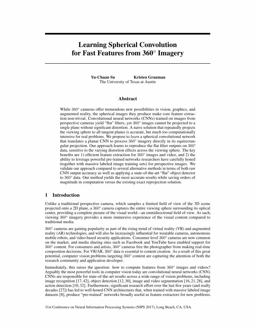
Figure 3: Spherical convolution. The kernel weight in spherical convolution is tied only along each row of theequirectangular image (i.e., φ), and each kernel convolves along the row to generate 1D output. Note that thekernel size differs at different rows and layers, and it expands near the top and bottom of the image.

until the height of the Rf is larger than that of Kp in Ie. We then adjust the width kw similar to kh.Furthermore, we restrict the kernel size kh × kw to be smaller than an upper bound Uk. See Fig. 4.Because the Rf of Kl

e depends on Kl−1e , we search for the kernel size starting from the bottom layer.

It is important to relax the kernel from being square to being rectangular, because equirectangularprojection will expand content horizontally near the poles of the sphere (see Fig. 2). If we restrict thekernel to be square, the Rf of Ke can easily be taller but narrower than that of Kp which leads tooverfitting. It is also important to restrict the kernel size, otherwise the kernel can grow wide rapidlynear the poles and eventually cover the entire row. Although cutting off the kernel size may lead toinformation loss, the loss is not significant in practice because pixels in equirectangular projection donot distribute on the unit sphere uniformly; they are denser near the pole, and the pixels are by natureredundant in the region where the kernel size expands dramatically.

Besides adjusting the kernel sizes, we also adjust the number of pooling layers to match the pixelsize ∆θ in Ne and Np. We define ∆θe = 180°/He and restrict We = 2He to ensure ∆θe = ∆φe.Because max-pooling introduces shift invariance up to kw pixels in the image, which corresponds tokw ×∆θ degrees on the unit sphere, the physical meaning of max-pooling depends on the pixel size.Since the pixel size is usually larger in Ie and max-pooling increases the pixel size by a factor of kw,we remove the pooling layer in Ne if ∆θe ≥ ∆θp.

Fig. 3 illustrates how spherical convolution differs from ordinary CNN. Note that we approximateone layer in Np by one layer in Ne, so the number of layers and output channels in each layer isexactly the same as the target network. However, this does not have to be the case. For example,we could use two or more layers to approximate each layer in Np. Although doing so may improveaccuracy, it would also introduce significant overhead, so we stick with the one-to-one mapping.

3.3 Training Process

Given the goal in Eq. 2 and the architecture described in Sec. 3.2, we would like to learn the networkNe by minimizing the L2 loss E[(Ne(Ie) − Np(Is))

2]. However, the network converges slowly,possibly due to the large number of parameters. Instead, we propose a kernel-wise pre-trainingprocess that disassembles the network and initially learns each kernel independently.

To perform kernel-wise pre-training, we further require Ne to generate the same intermediate repre-sentation as Np in all layers l:

N le(Ie)[x, y] ≈ N l

p(Is)[θ, φ] ∀l ∈ Ne. (3)

Given Eq. 3, every layer l ∈ Ne is independent of each other. In fact, every kernel is independent andcan be learned separately. We learn each kernel by taking the “ground truth” value of the previouslayer N l−1

p (Is) as input and minimizing the L2 loss E[(N le(Ie)−N l

p(Is))2], except for the first layer.

Note that N lp refers to the convolution output of layer l before applying any non-linear operation,

e.g. ReLU, max-pooling, etc. It is important to learn the target value before applying ReLU becauseit provides more information. We combine the non-linear operation with Kl+1

e during kernel-wisepre-training, and we use dilated convolution [39] to increase the Rf size instead of performingmax-pooling on the input feature map.

For the first convolution layer, we derive the analytic solution directly. The projection operator P islinear in the pixels in equirectangular projection: P(Is, n)[x, y] =

∑ij cijIe[i, j], for coefficients cij

5

Receptive FieldTarget Network Np Perspective Projection

(Inverse)

Receptive FieldNetwork Ne

No

kw× kh > Uk

kw

khIncreasekh

No

Yes>

Yes

Output kh

Target Kernel Kp

Kernel Ke

Figure 4: Method to select the kernel height kh. We project the receptive field of the target kernel to equirectan-gular projection Ie and increase kh until it is taller than the target kernel in Ie. The kernel width kw is determinedusing the same procedure after kh is set. We restrict the kernel size kw × kh by an upper bound Uk.

from, e.g., bilinear interpolation. Because convolution is a weighted sum of input pixels Kp ∗ Ip =∑xy wxyIp[x, y], we can combine the weight wxy and interpolation coefficient cij as a single

convolution operator:

K1p ∗ Is[θ, φ] =

∑xy

wxy

∑ij

cijIe[i, j] =∑ij

(∑xy

wxycij

)Ie[i, j] = K1

e ∗ Ie. (4)

The output value of N1e will be exact and requires no learning. Of course, the same is not possible for

l > 1 because of the non-linear operations between layers.

After kernel-wise pre-training, we can further fine-tune the network jointly across layers and kernelsby minimizing the L2 loss of the final output. Because the pre-trained kernels cannot fully recoverthe intermediate representation, fine-tuning can help to adjust the weights to account for residualerrors. We ignore the constraint introduced in Eq. 3 when performing fine-tuning. Although Eq. 3is necessary for kernel-wise pre-training, it restricts the expressive power of Ne and degrades theperformance if we only care about the final output. Nevertheless, the weights learned by kernel-wisepre-training are a very good initialization in practice, and we typically only need to fine-tune thenetwork for a few epochs.

One limitation of SPHCONV is that it cannot handle very close objects that span a large FOV. Becausethe goal of SPHCONV is to reproduce the behavior of models trained on perspective images, thecapability and performance of the model is bounded by the target model Np. However, perspectivecameras can only capture a small portion of a very close object in the FOV, and very close objects areusually not available in the training data of the target model Np. Therefore, even though 360° imagesoffer a much wider FOV, SPHCONV inherits the limitations of Np, and may not recognize very closelarge objects. Another limitation of SPHCONV is the resulting model size. Because it unties thekernel weights along θ, the model size grows linearly with the equirectangular image height. Themodel size can easily grow to tens of gigabytes as the image resolution increases.

4 ExperimentsTo evaluate our approach, we consider both the accuracy of its convolutions as well as its applicabilityfor object detections in 360° data. We use the VGG architecture3 and the Faster-RCNN [30] model asour target network Np. We learn a network Ne to produce the topmost (conv5_3) convolution output.

Datasets We use two datasets: Pano2Vid for training, and Pano2Vid and PASCAL for testing.

Pano2Vid: We sample frames from the 360° videos in the Pano2Vid dataset [35] for both trainingand testing. The dataset consists of 86 videos crawled from YouTube using four keywords: “Hiking,”“Mountain Climbing,” “Parade,” and “Soccer”. We sample frames at 0.05fps to obtain 1,056 framesfor training and 168 frames for testing. We use “Mountain Climbing” for testing and others fortraining, so the training and testing frames are from disjoint videos. See Supp. for sampling process.Because the supervision is on a per pixel basis, this corresponds to N ×We ×He ≈ 250M (noni.i.d.) samples. Note that most object categories targeted by the Faster-RCNN detector do not appearin Pano2Vid, meaning that our experiments test the content-independence of our approach.

PASCAL VOC: Because the target model was originally trained and evaluated on PASCAL VOC 2007,we “360-ify” it to evaluate the object detector application. We test with the 4,952 PASCAL images,which contain 12,032 bounding boxes. We transform them to equirectangular images as if they

3https://github.com/rbgirshick/py-faster-rcnn

6

originated from a 360° camera. In particular, each object bounding box is backprojected to 3 differentscales {0.5R, 1.0R, 1.5R} and 5 different polar angles θ∈{36°, 72°, 108°, 144°, 180°} on the 360°image sphere using the inverse perspective projection, whereR is the resolution of the target network’sRf. Regions outside the bounding box are zero-padded. See Supp. for details. Backprojection allowsus to evaluate the performance at different levels of distortion in the equirectangular projection.

Metrics We generate the output widely used in the literature (conv5_3) and evaluate it with thefollowing metrics.

Network output error measures the difference between Ne(Ie) and Np(Is). In particular, we reportthe root-mean-square error (RMSE) over all pixels and channels. For PASCAL, we measure the errorover the Rf of the detector network.

Detector network performance measures the performance of the detector network in Faster-RCNNusing multi-class classification accuracy. We replace the ROI-pooling in Faster-RCNN by poolingover the bounding box in Ie. Note that the bounding box is backprojected to equirectangular projectionand is no longer a square region.

Proposal network performance evaluates the proposal network in Faster-RCNN using averageIntersection-over-Union (IoU). For each bounding box centered at n, we project the conv5_3 outputto the tangent plane n using P and apply the proposal network at the center of the bounding box onthe tangent plane. Given the predicted proposals, we compute the IoUs between foreground proposalsand the bounding box and take the maximum. The IoU is set to 0 if there is no foreground proposal.Finally, we average the IoU over bounding boxes.

We stress that our goal is not to build a new object detector; rather, we aim to reproduce the behaviorof existing 2D models on 360° data with lower computational cost. Thus, the metrics capture howaccurately and how quickly we can replicate the exact solution.

Baselines We compare our method with the following baselines.• EXACT — Compute the true target value Np(Is)[θ, φ] for every pixel. This serves as an upper

bound in performance and does not consider the computational cost.• DIRECT — Apply Np on Ie directly. We replace max-pooling with dilated convolution to produce

a full resolution output. This is Strategy I in Fig. 1 and is used in 360° video analysis [19, 26].• INTERP — Compute Np(Is)[θ, φ] every S-pixels and interpolate the values for the others. We setS such that the computational cost is roughly the same as our SPHCONV. This is a more efficientvariant of Strategy II in Fig. 1.• PERSPECT — Project Is onto a cube map [2] and then apply Np on each face of the cube, which is

a perspective image with 90° FOV. The result is backprojected to Ie to obtain the feature on Ie.We use W=960 for the cube map resolution so ∆θ is roughly the same as Ip. This is a secondvariant of Strategy II in Fig. 1 used in PanoContext [41].

SPHCONV variants We evaluate three variants of our approach:• OPTSPHCONV — To compute the output for each layer l, OPTSPHCONV computes the exact

output for layer l−1 using Np(Is) then applies spherical convolution for layer l. OPTSPHCONVserves as an upper bound for our approach, where it avoids accumulating any error across layers.

• SPHCONV-PRE — Uses the weights from kernel-wise pre-training directly without fine-tuning.• SPHCONV — The full spherical convolution with joint fine-tuning of all layers.

Implementation details We set the resolution of Ie to 640×320. For the projection operator P , wemap α=65.5° to W=640 pixels following SUN360 [38]. The pixel size is therefore ∆θe=360°/640for Ie and ∆θp=65.5°/640 for Ip. Accordingly, we remove the first three max-pooling layers soNe has only one max-pooling layer following conv4_3. The kernel size upper bound Uk=7 × 7following the max kernel size in VGG. We insert batch normalization for conv4_1 to conv5_3. SeeSupp. for details.

4.1 Network output accuracy and computational cost

Fig. 5a shows the output error of layers conv3_3 and conv5_3 on the Pano2Vid [35] dataset (seeSupp. for similar results on other layers.). The error is normalized by that of the mean predictor. Weevaluate the error at 5 polar angles θ uniformly sampled from the northern hemisphere, since error isroughly symmetric with the equator.

7

18◦ 36◦ 54◦ 72◦ 90◦0

1

2

conv3 3 RMSE

18◦ 36◦ 54◦ 72◦ 90◦0

1

2

conv5 3 RMSE

θ

DirectInterpPerspectiveExactOptSphConvSphConv-PreSphConv

(a) Network output errors vs. polar angle

101 102 1030.4

0.5

0.6

0.7

0.8Accuracy

0 2 4 60

0.5

1

1.5conv5 3 RMSE

Tera-MACs

(b) Cost vs. accuracyFigure 5: (a) Network output error on Pano2Vid; lower is better. Note the error of EXACT is 0 by definition.Our method’s convolutions are much closer to the exact solution than the baselines’. (b) Computational costvs. accuracy on PASCAL. Our approach yields accuracy closest to the exact solution while requiring orders ofmagnitude less computation time (left plot). Our cost is similar to the other approximations tested (right plot).Plot titles indicate the y-labels, and error is measured by root-mean-square-error (RMSE).

Figure 6: Three AlexNet conv1 kernels (left squares) and their corresponding four SPHCONV-PRE kernels atθ ∈ {9°, 18°, 36°, 72°} (left to right).

First we discuss the three variants of our method. OPTSPHCONV performs the best in all layersand θ, validating our main idea of spherical convolution. It performs particularly well in the lowerlayers, because the Rf is larger in higher layers and the distortion becomes more significant. Overall,SPHCONV-PRE performs the second best, but as to be expected, the gap with OPTCONV becomeslarger in higher layers because of error propagation. SPHCONV outperforms SPHCONV-PRE inconv5_3 at the cost of larger error in lower layers (as seen here for conv3_3). It also has larger errorat θ=18° for two possible reasons. First, the learning curve indicates that the network learns moreslowly near the pole, possibly because the Rf is larger and the pixels degenerate. Second, we optimizethe joint L2 loss, which may trade the error near the pole with that at the center.

Comparing to the baselines, we see that ours achieves lowest errors. DIRECT performs the worstamong all methods, underscoring that convolutions on the flattened sphere—though fast—are inade-quate. INTERP performs better than DIRECT, and the error decreases in higher layers. This is becausethe Rf is larger in the higher layers, so the S-pixel shift in Ie causes relatively smaller changes inthe Rf and therefore the network output. PERSPECTIVE performs similarly in different layers andoutperforms INTERP in lower layers. The error of PERSPECTIVE is particularly large at θ=54°, whichis close to the boundary of the perspective image and has larger perspective distortion.

Fig. 5b shows the accuracy vs. cost tradeoff. We measure computational cost by the number ofMultiply-Accumulate (MAC) operations. The leftmost plot shows cost on a log scale. Here wesee that EXACT—whose outputs we wish to replicate—is about 400 times slower than SPHCONV,and SPHCONV approaches EXACT’s detector accuracy much better than all baselines. The secondplot shows that SPHCONV is about 34% faster than INTERP (while performing better in all metrics).PERSPECTIVE is the fastest among all methods and is 60% faster than SPHCONV, followed byDIRECT which is 23% faster than SPHCONV. However, both baselines are noticeably inferior inaccuracy compared to SPHCONV.

To visualize what our approach has learned, we learn the first layer of the AlexNet [25] modelprovided by the Caffe package [23] and examine the resulting kernels. Fig. 6 shows the originalkernel Kp and the corresponding kernels Ke at different polar angles θ. Ke is usually the re-scaledversion of Kp, but the weights are often amplified because multiple pixels in Kp fall to the samepixel in Ke like the second example. We also observe situations where the high frequency signal inthe kernel is reduced, like the third example, possibly because the kernel is smaller. Note that welearn the first convolution layer for visualization purposes only, since l = 1 (only) has an analyticsolution (cf. Sec 3.3). See Supp. for the complete set of kernels.

4.2 Object detection and proposal accuracyHaving established our approach provides accurate and efficient Ne convolutions, we now examinehow important that accuracy is to object detection on 360° inputs. Fig. 7a shows the result of theFaster-RCNN detector network on PASCAL in 360° format. OPTSPHCONV performs almost as wellas EXACT. The performance degrades in SPHCONV-PRE because of error accumulation, but it still

8

18◦ 36◦ 54◦ 72◦ 90◦0.2

0.4

0.6

0.8Accuracy

18◦ 36◦ 54◦ 72◦ 90◦0

0.5

1

1.5

2Output RMSE

DirectInterpPerspectiveExactOptSphConvSphConv-PreSphConv

(a) Detector network performance.18◦ 36◦ 54◦ 72◦ 90◦0

0.1

0.2

0.3

IoU

Scale = 0.5R

18◦ 36◦ 54◦ 72◦ 90◦0

0.1

0.2

0.3

Scale = 1.0R

(b) Proposal network accuracy (IoU).Figure 7: Faster-RCNN object detection accuracy on a 360° version of PASCAL across polar angles θ, for boththe (a) detector network and (b) proposal network. R refers to the Rf of Np. Best viewed in color.

Figure 8: Object detection examples on 360° PASCAL test images. Images show the top 40% of equirectangularprojection; black regions are undefined pixels. Text gives predicted label, multi-class probability, and IoU, resp.Our method successfully detects objects undergoing severe distortion, some of which are barely recognizableeven for a human viewer.

significantly outperforms DIRECT and is better than INTERP and PERSPECTIVE in most regions.Although joint training (SPHCONV) improves the output error near the equator, the error is larger nearthe pole which degrades the detector performance. Note that the Rf of the detector network spansmultiple rows, so the error is the weighted sum of the error at different rows. The result, togetherwith Fig. 5a, suggest that SPHCONV reduces the conv5_3 error in parts of the Rf but increases it atthe other parts. The detector network needs accurate conv5_3 features throughout the Rf in order togenerate good predictions.

DIRECT again performs the worst. In particular, the performance drops significantly at θ=18°,showing that it is sensitive to the distortion. In contrast, INTERP performs better near the polebecause the samples are denser on the unit sphere. In fact, INTERP should converge to EXACT at thepole. PERSPECTIVE outperforms INTERP near the equator but is worse in other regions. Note thatθ∈{18°, 36°} falls on the top face, and θ=54° is near the border of the face. The result suggests thatPERSPECTIVE is still sensitive to the polar angle, and it performs the best when the object is near thecenter of the faces where the perspective distortion is small.

Fig. 7b shows the performance of the object proposal network for two scales (see Supp. for more).Interestingly, the result is different from the detector network. OPTSPHCONV still performs almostthe same as EXACT, and SPHCONV-PRE performs better than baselines. However, DIRECT nowoutperforms other baselines, suggesting that the proposal network is not as sensitive as the detectornetwork to the distortion introduced by equirectangular projection. The performance of the methodsis similar when the object is larger (right plot), even though the output error is significantly different.The only exception is PERSPECTIVE, which performs poorly for θ∈{54°, 72°, 90°} regardless of theobject scale. It again suggests that objectness is sensitive to the perspective image being sampled.

Fig. 8 shows examples of objects successfully detected by our approach in spite of severe distortions.See Supp. for more examples.

5 ConclusionWe propose to learn spherical convolutions for 360° images. Our solution entails a new form ofdistillation across camera projection models. Compared to current practices for feature extraction on360° images/video, spherical convolution benefits efficiency by avoiding performing multiple per-spective projections, and it benefits accuracy by adapting kernels to the distortions in equirectangularprojection. Results on two datasets demonstrate how it successfully transfers state-of-the-art visionmodels from the realm of limited FOV 2D imagery into the realm of omnidirectional data.

Future work will explore SPHCONV in the context of other dense prediction problems like segmenta-tion, as well as the impact of different projection models within our basic framework.

9

References[1] https://facebook360.fb.com/editing-360-photos-injecting-metadata/.[2] https://code.facebook.com/posts/1638767863078802/under-the-hood-building-360-video/.[3] J. Ba and R. Caruana. Do deep nets really need to be deep? In NIPS, 2014.[4] A. Barre, A. Flocon, and R. Hansen. Curvilinear perspective, 1987.[5] C. Bucilua, R. Caruana, and A. Niculescu-Mizil. Model compression. In ACM SIGKDD, 2006.[6] T. Cohen, M. Geiger, J. Köhler, and M. Welling. Convolutional networks for spherical signals. arXiv

preprint arXiv:1709.04893, 2017.[7] J. Dai, H. Qi, Y. Xiong, Y. Li, G. Zhang, H. Hu, and Y. Wei. Deformable convolutional networks. In ICCV,

2017.[8] J. Deng, W. Dong, R. Socher, L. Li, and L. Fei-Fei. Imagenet: a large-scale hierarchical image database.

In CVPR, 2009.[9] M. Everingham, S. M. A. Eslami, L. Van Gool, C. K. I. Williams, J. Winn, and A. Zisserman. The pascal

visual object classes challenge: A retrospective. International Journal of Computer Vision, 111(1):98–136,Jan. 2015.

[10] C. Feichtenhofer, A. Pinz, and A. Zisserman. Convolutional two-stream network fusion for video actionrecognition. In CVPR, 2016.

[11] A. Furnari, G. M. Farinella, A. R. Bruna, and S. Battiato. Affine covariant features for fisheye distortionlocal modeling. IEEE Transactions on Image Processing, 26(2):696–710, 2017.

[12] R. Girshick, J. Donahue, T. Darrell, and J. Malik. Rich feature hierarchies for accurate object detectionand semantic segmentation. In CVPR, 2014.

[13] S. Gupta, J. Hoffman, and J. Malik. Cross modal distillation for supervision transfer. In CVPR, 2016.[14] P. Hansen, P. Corke, W. Boles, and K. Daniilidis. Scale-invariant features on the sphere. In ICCV, 2007.[15] P. Hansen, P. Corket, W. Boles, and K. Daniilidis. Scale invariant feature matching with wide angle images.

In IROS, 2007.[16] K. He, G. Gkioxari, P. Dollár, and R. Girshick. Mask r-cnn. In ICCV, 2017.[17] K. He, X. Zhang, S. Ren, and J. Sun. Deep residual learning for image recognition. In CVPR, 2016.[18] G. Hinton, O. Vinyals, and J. Dean. Distilling the knowledge in a neural network. arXiv preprint

arXiv:1503.02531, 2015.[19] H.-N. Hu, Y.-C. Lin, M.-Y. Liu, H.-T. Cheng, Y.-J. Chang, and M. Sun. Deep 360 pilot: Learning a deep

agent for piloting through 360° sports video. In CVPR, 2017.[20] M. Jaderberg, K. Simonyan, A. Zisserman, et al. Spatial transformer networks. In NIPS, 2015.[21] S. Jain, B. Xiong, and K. Grauman. Fusionseg: Learning to combine motion and appearance for fully

automatic segmentation of generic objects in video. In CVPR, 2017.[22] Y. Jeon and J. Kim. Active convolution: Learning the shape of convolution for image classification. In

CVPR, 2017.[23] Y. Jia, E. Shelhamer, J. Donahue, S. Karayev, J. Long, R. Girshick, S. Guadarrama, and T. Darrell. Caffe:

Convolutional architecture for fast feature embedding. In ACM MM, 2014.[24] R. Khasanova and P. Frossard. Graph-based classification of omnidirectional images. arXiv preprint

arXiv:1707.08301, 2017.[25] A. Krizhevsky, I. Sutskever, and G. Hinton. Imagenet classification with deep convolutional neural

networks. In NIPS, 2012.[26] W.-S. Lai, Y. Huang, N. Joshi, C. Buehler, M.-H. Yang, and S. B. Kang. Semantic-driven generation of

hyperlapse from 360° video. IEEE Transactions on Visualization and Computer Graphics, PP(99):1–1,2017.

[27] Y. LeCun, L. Bottou, Y. Bengio, and P. Haffner. Gradient-based learning applied to document recognition.In Proc. of the IEEE, 1998.

[28] J. Long, E. Shelhamer, and T. Darrell. Fully convolutional networks for semantic segmentation. In CVPR,2015.

[29] E. Parisotto, J. Ba, and R. Salakhutdinov. Actor-mimic: Deep multitask and transfer reinforcement learning.In ICLR, 2016.

[30] S. Ren, K. He, R. Girshick, and J. Sun. Faster r-cnn: Towards real-time object detection with regionproposal networks. In NIPS, 2015.

[31] A. Romero, N. Ballas, S. E. Kahou, A. Chassang, C. Gatta, and Y. Bengio. Fitnets: Hints for thin deepnets. In ICLR, 2015.

[32] K. Simonyan and A. Zisserman. Two-stream convolutional networks for action recognition in videos. InNIPS, 2014.

[33] K. Simonyan and A. Zisserman. Very deep convolutional networks for large-scale image recognition. InICLR, 2015.

[34] Y.-C. Su and K. Grauman. Making 360° video watchable in 2d: Learning videography for click freeviewing. In CVPR, 2017.

10

[35] Y.-C. Su, D. Jayaraman, and K. Grauman. Pano2vid: Automatic cinematography for watching 360° videos.In ACCV, 2016.

[36] D. Tran, L. Bourdev, R. Fergus, L. Torresani, and M. Paluri. Learning spatiotemporal features with 3dconvolutional networks. In ICCV, 2015.

[37] Y.-X. Wang and M. Hebert. Learning to learn: Model regression networks for easy small sample learning.In ECCV, 2016.

[38] J. Xiao, K. A. Ehinger, A. Oliva, and A. Torralba. Recognizing scene viewpoint using panoramic placerepresentation. In CVPR, 2012.

[39] F. Yu and V. Koltun. Multi-scale context aggregation by dilated convolutions. In ICLR, 2016.[40] L. Zelnik-Manor, G. Peters, and P. Perona. Squaring the circle in panoramas. In ICCV, 2005.[41] Y. Zhang, S. Song, P. Tan, and J. Xiao. Panocontext: A whole-room 3d context model for panoramic scene

understanding. In ECCV, 2014.[42] B. Zhou, A. Lapedriza, J. Xiao, A. Torralba, and A. Oliva. Learning deep features for scene recognition

using places database. In NIPS, 2014.

11