learning sentinel-2 spectral dynamics for long-run
TRANSCRIPT
HAL Id: hal-03265010https://hal-imt-atlantique.archives-ouvertes.fr/hal-03265010
Submitted on 18 Jun 2021
HAL is a multi-disciplinary open accessarchive for the deposit and dissemination of sci-entific research documents, whether they are pub-lished or not. The documents may come fromteaching and research institutions in France orabroad, or from public or private research centers.
L’archive ouverte pluridisciplinaire HAL, estdestinée au dépôt et à la diffusion de documentsscientifiques de niveau recherche, publiés ou non,émanant des établissements d’enseignement et derecherche français ou étrangers, des laboratoirespublics ou privés.
Learning Sentinel-2 Spectral Dynamics for Long-runPredictions using Residual Neural Networks
Joaquim Estopinan, Guillaume Tochon, Lucas Drumetz
To cite this version:Joaquim Estopinan, Guillaume Tochon, Lucas Drumetz. Learning Sentinel-2 Spectral Dynamics forLong-run Predictions using Residual Neural Networks. EUSIPCO 2021: 29th European Signal Pro-cessing Conference, Aug 2021, Dublin (virtual), Ireland. �10.23919/EUSIPCO54536.2021.9616304�.�hal-03265010�

Learning Sentinel-2 Spectral Dynamics forLong-run Predictions using Residual Neural
NetworksJoaquim Estopinan
EPITA Research and DevelopmentLaboratory (LRDE)
Le Kremlin-Bicetre, [email protected]
Guillaume TochonEPITA Research and Development
Laboratory (LRDE)Le Kremlin-Bicetre, France
Lucas DrumetzLab-STICC, UMR CNRS 6285
IMT AtlantiqueBrest, France
Abstract—Making the most of multispectral image time-seriesis a promising but still relatively under-explored research di-rection because of the complexity of jointly analyzing spatial,spectral and temporal information. Capturing and characterizingtemporal dynamics is one of the important and challenging issues.Our new method paves the way to capture real data dynamics andshould eventually benefit applications like unmixing or classifi-cation. Dealing with time-series dynamics classically requires theknowledge of a dynamical model and an observation model. Theformer may be incorrect or computationally hard to handle, thusmotivating data-driven strategies aiming at learning dynamicsdirectly from data. In this paper, we adapt neural networkarchitectures to learn periodic dynamics of both simulated andreal multispectral time-series. We emphasize the necessity ofchoosing the right state variable to capture periodic dynamicsand show that our models can reproduce the average seasonaldynamics of vegetation using only one year of training data.
Index Terms—remote sensing, multispectral images, time-series, spectral dynamics, recurrent neural networks
I. INTRODUCTION
The Sentinel-2 mission is part of the European Earthobservation project Copernicus, a program jointly led by theEuropean Space Agency (ESA) and the European Commis-sion. It intends to provide authorities and interested actors withopen multispectral data reflecting Earth surface changes, withproper natural resources management as end goal. The missionconsists in two polar-orbiting satellites synchronized on thesame sun orbit, and diametrically opposite to one another. Aseach Sentinel-2 satellite has a temporal revisit of ten days, thecommon temporal revisit of a given location on earth underthe same viewing conditions goes down to five days [1].The Sentinel-2 mission (or the soon to be launched pendinghyperspectral EnMAP mission [2]) gives access to spectraltime-series with a high temporal revisit. Such multidimen-sional data require a particular care to extract their richinformation, but proved to greatly increase carried out taskresults when processed successfully [3]–[5]. The automaticlearning of spectral dynamics would provide a new spectral
This work has been supported by the Programme National de TeledetectionSpatiale (PNTS), grant n◦PNTS-2019-4.
insight on the observed areas. It could benefit a large panelof applications such as spectral unmixing, anomaly detection,data assimilation [6] and predictions on vulnerable speciesconservation status [7]. It was proven in [8] that knowingspectral dynamics improves an endmember estimation task onsynthetic data.In the observed scenes, pure materials of interest are varyingthrough time in their spectral signature or/and their spatialextent because of seasonal changes for instance. Reference [9]showed that a state-space model is convenient to model theseevolutions. For a given material described by a n-dimensionalstate variable Xt, the state equation of the model is given byan ordinary differential equation (ODE) when only temporalvariations of the spectra are considered:
dXt
dt= F(Xt) + ηt (1)
where F is the dynamical operator and ηt an error accountingfor both noise and model approximation. Our objective isthereby to directly learn from data these dynamics withspecific neural network (NN) architectures [8].The contribution of this article is threefold: (i) a particularstate variable describing spectral signatures is shown efficientto learn periodic dynamics with residual neural networks(ResNets), (ii) long-run predictions on synthetic data showthat the developed architecture is clearly more adapted for suchtask than a long short-term memory (LSTM) [10] architecture,(iii) first results on real data demonstrate the potential of ourmethod for applications like classification or unmixing.In the following, Section II focuses on methods and NNsto learn spectral dynamics. Then, Sections III and IV intro-duce conducted experiments and results on synthetic and realSentinel-2 data, respectively. Finally, Section V gathers ourconclusions on this work and its implications.
II. DYNAMICS LEARNING
A. ResNet architecture
Recurrent neural networks (RNNs) architectures, such asLSTM networks [10], are natural candidates when it comes
arX
iv:2
011.
0874
6v2
[ee
ss.I
V]
19
Mar
202
1
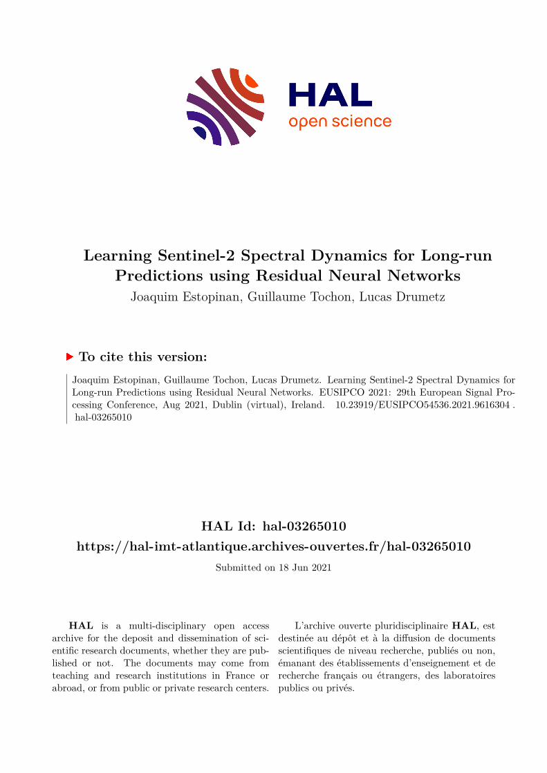
(a) Euler (b) Runge-Kutta 4
Fig. 1. ResNets architectures implementing (a) Euler and (b) Runge-Kutta integration schemes.
to learning and processing time-series data. Among RNNsarchitectures, ResNets with shared weights across layers haverecently been proven to be particularly adapted to estimatedynamical operators [11]. Using them allows to reformulatethe problem of learning an input/output relationship to thelearning of a deviation from the identity [11], [12], makingthem suited to process data generated by differential equations.Mathematically, we assume that spectral signatures can be ob-tained by the following equation inherited from the integrationof the ODE (1):
st+h = st + hδ(st), (2)
st being the pixel L-dimensional reflectance at time-step (t), Lis the number of exploited spectral bands, δ is the infinitesimaloperator of the integrated ODE and h is the integration step(herafter set to 1 without loss of generality). In the ResNettypical architecture, a hard-cabled skip connection constrainsthe learning of the difference between st+h and st, see Fig. 1(a). The problem is thus shifted to the learning of the infinites-imal operator δ. To achieve this, two numerical integrationprocedures are classically considered: the first-order Eulermethod and the more refined fourth-order Runge-Kutta 4(RK4) method. These numerical integration schemes are hard-coded in the architectures. The ResNets are then learningthe ODE through the weights attributed to the infinitesimaloperator δ.
B. Euler and Runge-Kutta 4 integration schemes
The classical first-order Euler method consists in approxi-mating δ by the temporal derivative of the targeted function:
st+1 = st + s′t (3)
An approximation of s′t is therefore learned through the sharedweights of δ, see Fig. 1 (a) (the rationale for the dimension 2Lis further explained in Section II-C). The two layers encodingδ are distributed through the whole time-series. The local error,i.e. the error per step, is on the order O(h2) [13].The architecture of the RK4 integration scheme is displayedby Fig. 1 (b). Here, the approximation of δ is given by aweighted average of four slopes taken at the beginning, themiddle and the end of the integration step (their respectiveweighting coefficients being k1, k2, k3 and k4), and the four
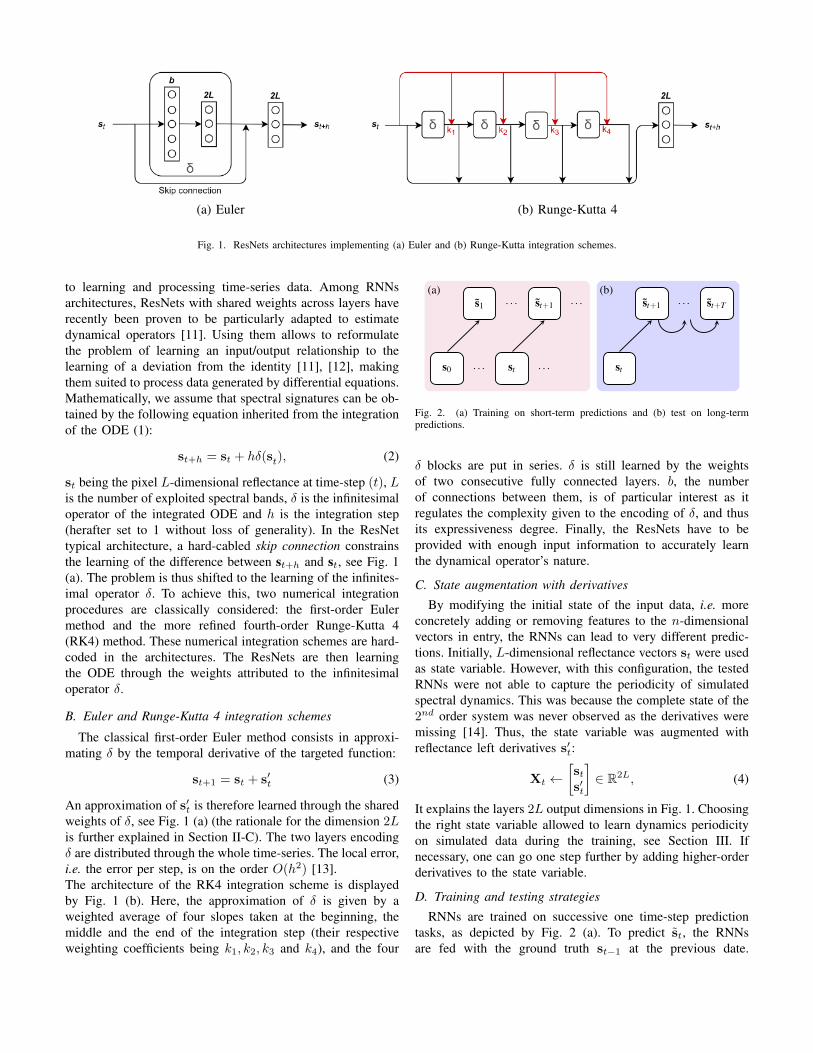
(a)
s0 . . . st . . .
s1 . . . st+1 . . .(b)
st
st+1 . . . st+T
Fig. 2. (a) Training on short-term predictions and (b) test on long-termpredictions.
δ blocks are put in series. δ is still learned by the weightsof two consecutive fully connected layers. b, the numberof connections between them, is of particular interest as itregulates the complexity given to the encoding of δ, and thusits expressiveness degree. Finally, the ResNets have to beprovided with enough input information to accurately learnthe dynamical operator’s nature.
C. State augmentation with derivatives
By modifying the initial state of the input data, i.e. moreconcretely adding or removing features to the n-dimensionalvectors in entry, the RNNs can lead to very different predic-tions. Initially, L-dimensional reflectance vectors st were usedas state variable. However, with this configuration, the testedRNNs were not able to capture the periodicity of simulatedspectral dynamics. This was because the complete state of the2nd order system was never observed as the derivatives weremissing [14]. Thus, the state variable was augmented withreflectance left derivatives s′t:
Xt ←[sts′t
]∈ R2L, (4)
It explains the layers 2L output dimensions in Fig. 1. Choosingthe right state variable allowed to learn dynamics periodicityon simulated data during the training, see Section III. Ifnecessary, one can go one step further by adding higher-orderderivatives to the state variable.
D. Training and testing strategies
RNNs are trained on successive one time-step predictiontasks, as depicted by Fig. 2 (a). To predict st, the RNNsare fed with the ground truth st−1 at the previous date.
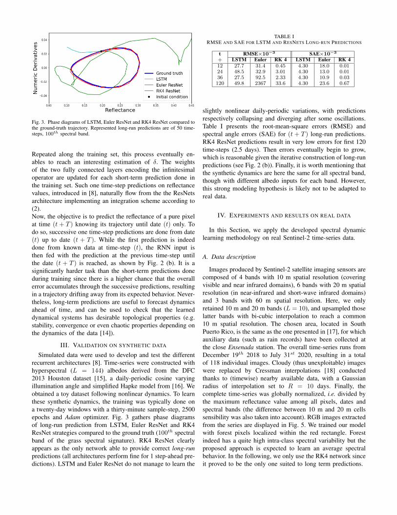
Fig. 3. Phase diagrams of LSTM, Euler ResNet and RK4 ResNet compared tothe ground-truth trajectory. Represented long-run predictions are of 50 time-steps, 100th spectral band.
Repeated along the training set, this process eventually en-ables to reach an interesting estimation of δ. The weightsof the two fully connected layers encoding the infinitesimaloperator are updated for each short-term prediction done inthe training set. Such one time-step predictions on reflectancevalues, introduced in [8], naturally flow from the the ResNetsarchitecture implementing an integration scheme according to(2).Now, the objective is to predict the reflectance of a pure pixelat time (t + T ) knowing its trajectory until date (t) only. Todo so, successive one time-step predictions are done from date(t) up to date (t + T ). While the first prediction is indeeddone from known data at time-step (t), the RNN input isthen fed with the prediction at the previous time-step untilthe date (t + T ) is reached, as shown by Fig. 2 (b). It is asignificantly harder task than the short-term predictions doneduring training since there is a higher chance that the overallerror accumulates through the successive predictions, resultingin a trajectory drifting away from its expected behavior. Never-theless, long-term predictions are useful to forecast dynamicsahead of time, and can be used to check that the learneddynamical systems has desirable topological properties (e.g.stability, convergence or even chaotic properties depending onthe dynamics of the data [14]).
III. VALIDATION ON SYNTHETIC DATA
Simulated data were used to develop and test the differentrecurrent architectures [8]. Time-series were constructed withhyperspectral (L = 144) albedos derived from the DFC2013 Houston dataset [15], a daily-periodic cosine varyingillumination angle and simplified Hapke model from [16]. Weobtained a toy dataset following nonlinear dynamics. To learnthese synthetic dynamics, the training was typically done ona twenty-day windows with a thirty-minute sample-step, 2500epochs and Adam optimizer. Fig. 3 gathers phase diagramsof long-run prediction from LSTM, Euler ResNet and RK4ResNet strategies compared to the ground truth (100th spectralband of the grass spectral signature). RK4 ResNet clearlyappears as the only network able to provide correct long-runpredictions (all architectures perform fine for 1 step-ahead pre-dictions). LSTM and Euler ResNet do not manage to learn the
TABLE IRMSE AND SAE FOR LSTM AND RESNETS LONG-RUN PREDICTIONS
t RMSE×10−3 SAE×10−3
+ LSTM Euler RK 4 LSTM Euler RK 412 27.7 31.4 0.45 4.30 18.0 0.0124 48.5 32.9 3.01 4.30 13.0 0.0136 27.5 92.5 2.33 4.30 10.9 0.03120 49.8 2367 33.6 4.30 23.6 0.67
slightly nonlinear daily-periodic variations, with predictionsrespectively collapsing and diverging after some oscillations.Table I presents the root-mean-square errors (RMSE) andspectral angle errors (SAE) for (t + T ) long-run predictions.RK4 ResNet predictions result in very low errors for first 120time-steps (2.5 days). Then errors eventually begin to grow,which is reasonable given the iterative construction of long-runpredictions (see Fig. 2 (b)). Finally, it is worth mentioning thatthe synthetic dynamics are here the same for all spectral band,though with different albedo inputs for each band. However,this strong modeling hypothesis is likely not to be adapted toreal data.
IV. EXPERIMENTS AND RESULTS ON REAL DATA
In this Section, we apply the developed spectral dynamiclearning methodology on real Sentinel-2 time-series data.
A. Data description
Images produced by Sentinel-2 satellite imaging sensors arecomposed of 4 bands with 10 m spatial resolution (coveringvisible and near infrared domains), 6 bands with 20 m spatialresolution (in near-infrared and short-wave infrared domains)and 3 bands with 60 m spatial resolution. Here, we onlyretained 10 m and 20 m bands (L = 10), and upsampled thoselatter bands with bi-cubic interpolation to reach a common10 m spatial resolution. The chosen area, located in SouthPuerto Rico, is the same as the one presented in [17], for whichauxiliary data (such as rain records) have been collected atthe close Ensenada station. The overall time-series runs fromDecember 19th 2018 to July 31st 2020, resulting in a totalof 118 individual images. Cloudy (thus unexploitable) imageswere replaced by Cressman interpolations [18] conductedthanks to (timewise) nearby available data, with a Gaussianradius of interpolation set to R = 10 days. Finally, thecomplete time-series was globally normalized, i.e. divided bythe maximum reflectance value among all pixels, dates andspectral bands (the difference between 10 m and 20 m cellssensibility was also taken into account). RGB images extractedfrom the series are displayed in Fig. 5. We trained our modelwith forest pixels localized within the red rectangle. Forestindeed has a quite high intra-class spectral variability but theproposed approach is expected to learn an average spectralbehavior. In the following, we only use the RK4 network sinceit proved to be the only one suited to long term predictions.

(a) 2019 Training data (b) 2020 Ground truth (c) 2020 Long-run prediction
Fig. 4. Temporal evolution of a forest spectrum (a) in 2019 (whole year), (b) in 2020 (half year) and (c) 2020 long-run prediction (whole year) for the samepixel.
Fig. 5. Four RGB images extracted from the time-series.
B. Obtained results
The training was done on 74 images ranging from December19th 2018 to December 19th 2019. Fig. 4 (a) displays thespectral evolution of a given forest pixel along those dates.Data included in the training set for a targeted pixel comprisedits four direct neighbors, leading to a batch size equal to 5.60000 epochs were needed with Adam optimizer and MSEloss function to reach convergence and realistic results. Thevalue given to b turned out to be a major success criterion,the architecture being fixed otherwise. We found out thataround 150 connections were optimal. Fig. 4 (b) representsthe evolution of the same pixel as in Fig. 4 (a) betweenJanuary 8th 2020 and July 31st 2020, serving as groundtruth. Finally, Fig. 4 (c) represents the long-run prediction over
73 dates (from January 8th 2020 to January 12th 2021) forthis pixel. The red portion accounts for predictions after the31st of July 2020, to easily compare prior predictions withthe ground truth. Predictions match the spectral decreasingtendency observable on the ground truth and peak predictionoccurs slightly later than in reality (just after the 31st ofJuly). RK4 ResNet nonetheless achieves to learn specific andperiodic patterns. The quality of the predictions decreaseswith time, but remains realistic. RMSE on January 18th isof 5.0 × 10⁻² and of 7.3 × 10⁻² on April 17th. Because ofthe peak late prediction, it finally reaches 1.3× 10⁻¹ on July26th.
V. CONCLUSION
In this work, we aimed at learning spectral dynamicspatterns and periodicity directly from data, without priorknowledge. We showed that, using the right state variable,the developed ResNet implementing RK4 integration schemesucceeded in that task on simulated and real time-seriesmultispectral data. Long-run predictions on synthetic datawere proven significantly better than with LSTM or EulerResNet, and realistic enough on a real multispectral time-seriesto capture seasonal variations in vegetation. Future researchavenues include optimizing hyperparameters and adding anenergy conservation constraint to further improve the results.A prior classification step on time-series to automaticallyintegrate in training set spectrally consistent zones is also apromising direction, as is the stochastic modeling of the spec-tral variability of vegetation (prediction of a probability densityinstead of point estimates). This work could eventually benefitapplications for space time interpolation of multispectral data,scene unmixing and forecasting problems among many others.

REFERENCES
[1] M. Drusch, U. Del Bello, S. Carlier, O. Colin, V. Fernandez, F. Gascon,B. Hoersch, C. Isola, P. Laberinti, P. Martimort, A. Meygret, F. Spoto,O. Sy, F. Marchese, and P. Bargellini, “Sentinel-2: ESA’s optical high-resolution mission for GMES operational services,” Remote Sensing ofEnvironment, vol. 120, pp. 25 – 36, 2012.
[2] L. Guanter, H. Kaufmann, K. Segl, S. Foerster, C. Rogass, S. Chabrillat,T. Kuester, A. Hollstein, G. Rossner, C. Chlebek, et al., “The EnMAPspaceborne imaging spectroscopy mission for earth observation,” RemoteSensing, vol. 7, no. 7, pp. 8830–8857, 2015.
[3] W. He and N. Yokoya, “Multi-temporal Sentinel-1 and -2 data fusionfor optical image simulation,” ISPRS International Journal of Geo-Information, vol. 7, no. 10, pp. 389, 2018.
[4] D. Tapete and F. Cigna, “Appraisal of opportunities and perspectives forthe systematic condition assessment of heritage sites with CopernicusSentinel-2 high-resolution multispectral imagery,” Remote Sensing, vol.10, no. 4, pp. 561–583, 2018.
[5] N. Yokoya, X. X. Zhu, and A. Plaza, “Multisensor coupled spectralunmixing for time-series analysis,” IEEE Transactions on Geoscienceand Remote Sensing, vol. 55, no. 5, pp. 2842–2857, 2017.
[6] G. Evensen, Data Assimilation: The Ensemble Kalman Filter, SpringerScience & Business Media, 2009.
[7] B. Cazorla, J. Cabello, J. Penas, P. Garcillan, D. A. Reyes, andD. Alcaraz-Segura, “Incorporating ecosystem functional diversity intogeographic conservation priorities using remotely sensed ecosystemfunctional types,” Ecosystems, pp. 1–17, 2020.
[8] L. Drumetz, M. Dalla Mura, G. Tochon, and R. Fablet, “Learningendmember dynamics in multitemporal hyperspectral data using a state-space model formulation,” 2020 IEEE International Conference onAcoustics, Speech and Signal Processing (ICASSP), pp. 2483–2487,2020.
[9] S. Henrot, J. Chanussot, and C. Jutten, “Dynamical spectral unmixingof multitemporal hyperspectral images,” IEEE Transactions on ImageProcessing, vol. 25, no. 7, pp. 3219–3232, 2016.
[10] S. Hochreiter and J. Schmidhuber, “Long short-term memory,” Neuralcomputation, vol. 9, pp. 1735–80, 1997.
[11] R. Fablet, S. Ouala, and C. Herzet, “Bilinear residual neural networkfor the identification and forecasting of dynamical systems,” EUSIPCO2018 : European Signal Processing Conference, pp. 1–5, 2018.
[12] Ricky T. Q. Chen, Yulia Rubanova, Jesse Bettencourt, and David KDuvenaud, “Neural ordinary differential equations,” in Advancesin Neural Information Processing Systems, S. Bengio, H. Wallach,H. Larochelle, K. Grauman, N. Cesa-Bianchi, and R. Garnett, Eds. 2018,vol. 31, pp. 6571–6583, Curran Associates, Inc.
[13] E. Hairer, C. Lubich, and M. Roche, The Numerical Solution ofDifferential-Algebraic Systems by Runge-Kutta Methods, vol. 1409,Springer, 2006.
[14] S. Ouala, D. Nguyen, L. Drumetz, B. Chapron, A. Pascual, F. Collard,L. Gaultier, and R. Fablet, “Learning latent dynamics for partially-observed chaotic systems,” Chaos: An Interdisciplinary Journal ofNonlinear Science, 2020.
[15] C. Debes, A. Merentitis, R. Heremans, J. Hahn, N. Frangiadakis,T. van Kasteren, W. Liao, R. Bellens, A. Pizurica, S. Gautama, et al.,“Hyperspectral and LiDAR data fusion: Outcome of the 2013 GRSSdata fusion contest,” IEEE Journal of Selected Topics in Applied EarthObservations and Remote Sensing, vol. 7, no. 6, pp. 2405–2418, 2014.
[16] L. Drumetz, J. Chanussot, and C. Jutten, “Spectral unmixing: Aderivation of the extended linear mixing model from the Hapke model,”IEEE Geoscience and Remote Sensing Letters, pp. 1–5, 2019.
[17] M. A. Goenaga, M. C. Torres-Madronero, M. Velez-Reyes, S. J. VanBloem, and J. D. Chinea, “Unmixing analysis of a time series ofhyperion images over the Guanica dry forest in Puerto Rico,” IEEEJournal of Selected Topics in Applied Earth Observations and RemoteSensing, vol. 6, no. 2, pp. 329–338, 2013.
[18] G. P. Cressman, “An operational objective analysis system,” MonthlyWeather Review, vol. 87, no. 10, pp. 367–374, 1959.