Free Sample

In this package, you will find: • The authors biography • A preview chapter from the book, Chapter 1 "Introduction to SciPy" • A synopsis of the book’s content • More information on Learning SciPy for Numerical and Scientific Computing

Second Edition

About the Authors Sergio J. Rojas G. is currently a full professor of physics at Universidad Simón Bolívar, Venezuela. Regarding his formal studies, in 1991, he earned a BS in physics with his thesis on numerical relativity from the Universidad de Oriente, Estado Sucre, Venezuela, and then, in 1998, he earned a PhD in physics from the Department of Physics at City College of the City University of New York, where he worked on the applications of fluid dynamics in the flow of fluids in porous media, gaining and developing since then a vast experience in programming as an aid to scientific research via Fortran77/90 and C/C++. In 2001, he also earned a master's degree in computational finance from the Oregon Graduate Institute of Science and Technology.

Sergio's teaching activities involve lecturing undergraduate and graduate physics courses at his home university, Universidad Simón Bolívar, Venezuela, including a course on Monte Carlo methods and another on computational finance. His research interests include physics education research, fluid flow in porous media, and the application of the theory of complex systems and statistical mechanics in financial engineering. More recently, Sergio has been involved in machine learning and its applications in science and engineering via the Python programming language.

I am deeply grateful to my mother, Eufemia del Valle Rojas González, a beloved woman whose given steps were always in favor of showing and upraising the best of a human being.

Erik A Christensen is a quant analyst/developer in finance and creative industries. He has a PhD from the Technical University of Denmark, with postdoctoral studies at the Levich Institute at the City College of the City University of New York and the Courant Institute of Mathematical Sciences at New York University. His interests in technology span from Python to F# and Cassandra/Spark. He is active in the meet-up communities in London!

I would like to thank my family and friends for their support during this work!

Francisco J. Blanco-Silva is the owner of a scientific consulting company-Tizona Scientific Solutions-and adjunct faculty in the Department of Mathematics of the University of South Carolina. He obtained his formal training as an applied mathematician at Purdue University. He enjoys problem solving, learning, and teaching. Being an avid programmer and blogger, when it comes to writing, he relishes finding that common denominator among his passions and skills and making it available to everyone. He coauthored Modeling Nanoscale Imaging in Electron Microscopy, Springer along with Peter Binev, Wolfgang Dahmen, and Thomas Vogt.

Learning SciPy for Numerical and Scientific Computing Second Edition While maintaining the main structure of the first edition, this revised edition of Learning SciPy for Numerical and Scientific Computing includes a set of companion IPython Notebooks. This will help students, researchers, and practitioners modify and incorporate in their own work, the set of tested code snippets that are presented in the book, as the pedagogical strategy. This will also show and illustrate the computing power that SciPy brings to the fingertips of anyone interested in performing numerical computation via the unique flexibility offered by the Python computer language.

We should mention, however, that the IPython Notebooks will make sense to anyone starting in the field only if they are read alongside the corresponding section in the book, helping you to develop skills in the use of SciPy to solve large scale numerical problems while gaining understanding of the conditions and limitations associated with the modules contained in SciPy. Certainly, the already knowledgeable reader will find pleasure as they encounter material they already know, but will be challenged to devise better ways to accomplish with the same level of clarity presented in the book with the many computational tasks used to illustrate the functionality of SciPy.

SciPy has been an integral part of the computational environment of choice for many scientists for years. One of our challenges today is to bring together professionals with different backgrounds, technologies, and expertise in software (from the pure mathematician, to the hardcore engineer) to contribute independent of their working environments.

SciPy in Python is a perfect platform to coordinate projects in a smooth, reliable, and coherent environment. It allows performing most tasks with ease; reason being that many dedicated software tools easily integrate with the core features of SciPy, therefore, interfacing with non-Python-based software packages and tools is becoming increasingly simple.

In summary, this book presents the most robust programming environment to date. We will show you how to use this system from basic manipulation of data, to a very detailed exposition through examples in different branches of science and engineering.

What This Book Covers Chapter 1, Introduction to SciPy, shows the benefits of using the combination of Python, NumPy, SciPy, and matplotlib as a programming environment for scientific purposes. You will learn how to install, test, and explore the environments, use them for quick computations, and figure out a few good ways to search for help. A brief introduction on how to open the companion IPython Notebooks that comes with this book is also presented.

Chapter 2, Working with the NumPy Array As a First Step to SciPy, explores in depth the creation and basic manipulation of the object array used by SciPy, as an overview of the NumPy libraries.

Chapter 3, SciPy for Linear Algebra, covers applications of SciPy to applications with large matrices, including solving systems or computation of eigenvalues and eigenvectors.

Chapter 4, SciPy for Numerical Analysis, is without a doubt one of the most interesting chapters in this book. It covers with great detail the defi nition and manipulation of functions (one or several variables), the extraction of their roots, extreme values (optimization), computation of derivatives, integration, interpolation, regression, and applications to the solution of ordinary differential equations.

Chapter 5, SciPy for Signal Processing, explores construction, acquisition, quality improvement, compression, and feature extraction of signals (in any dimension). It is covered with beautiful and interesting examples from the fi eld of image processing.

Chapter 6, SciPy for Data Mining, covers applications of SciPy for collection, organization, analysis, and interpretation of data, with examples taken from statistics and clustering.

Chapter 7, SciPy for Computational Geometry, explores the construction of triangulation of points, convex hulls, Voronoi diagrams, and applications, including the solving of the two dimensional Laplace Equation via the Finite Element Method in a rectangular grid. At this point in the book, it will be possible to combine techniques from all the previous chapters to show state-of-the-art research performed with ease with SciPy, and we will explore a few good examples from Material Science and Experimental Physics.

Chapter 8, Interaction with Other Languages, introduces one of the main strengths of SciPy-the ability to interact with other languages such as C/C++, Fortran, R, and MATLAB/Octave.

Introduction to SciPyThere is no doubt that the labor of scientists in the twenty-fi rst century is more comprehensive and interdisciplinary than in previous generations. Members of scientifi c communities connect in larger teams and work together on mission-oriented goals and across their fi elds. This paradigm on research is also refl ected in the computational resources employed by researchers. No longer are researchers restricted to one type of commercial software, operating system, or vendor, but inspired by open source contributions made available and tested by research institutions and open source communities; research work often spans over various platforms and technologies.

This book presents the highly-recognized open source programming environment till date — a system based on two libraries of the computer language Python: NumPy and SciPy. In the following sections, we will guide you through examples from science and engineering on the usage of this system.

What is SciPy?The ideal programming environment for computational mathematics enjoys the following characteristics:

• It must be based on a computer language that allows the user to work quickly and integrate systems effectively. Ideally, the computer language should be portable to all platforms: Windows, Mac OS X, Linux, Unix, Android, and so on. This is key to fostering cooperation among scientists with different resources and accessibilities. It must contain a powerful set of libraries that allow the acquisition, storing, and handling of large datasets in a simple and effective manner. This is central—allowing simulation and the employment of numerical computations at a large scale.

• Smooth integration with other computer languages, as well as third-party software.

Introduction to SciPy

[ 8 ]

• Besides running the compiled code, the programming environment should allow the possibility of interactive sessions as well as scripting capabilities for quick experimentation.

• Different coding paradigms should be supported—imperative, object-oriented, and/or functional coding styles.

• It should be an open source software, that allows user access to the raw data code, and allows the user to modify basic algorithms if so desired. With commercial software, the inclusion of the improved algorithms is applied at the discretion of the seller, and it usually comes at a cost of the end user. In the open source universe, the community usually performs these improvements and releases new versions as they are published—at no cost.

• The set of applications should not be restricted to mere numerical computations; it should be powerful enough to allow symbolic computations as well.

Among the best-known environments for numerical computations used by the scientifi c community is MATLAB, which is commercial, expensive, and which does not allow any tampering with the code. Maple and Mathematica are more geared towards symbolic computation, although they can match many of the numerical computations from MATLAB. These are, however, also commercial, expensive, and closed to modifi cations. A decent alternative to MATLAB and based on a similar mathematical engine is the GNU Octave system. Most of the MATLAB code is easily portable to Octave, which is open source. Unfortunately, the accompanying programming environment is not very user friendly, it is also very much restricted to numerical computations. One environment that combines the best of all worlds is Python with the open source libraries NumPy and SciPy for numerical operations. The fi rst property that attracts users to Python is, without a doubt, its code readability. The syntax is extremely clear and expressive. It has the advantage of supporting code written in different paradigms: object oriented, functional, or old school imperative. It allows packing of Python codes and to run them as standalone executable programs through the py2exe, pyinstaller, and cx_Freeze libraries, but it can also be used interactively or as a scripting language. This is a great advantage when developing tools for symbolic computation. Python has therefore been a fi rm competitor to Maple and Mathematica: the open source mathematics software Sage (System for Algebra and Geometry Experimentation).

NumPy is an open source extension to Python that adds support for multidimensional arrays of large sizes. This support allows the desired acquisition, storage, and complex manipulation of data mentioned previously. NumPy alone is a great tool to solve many numerical computations.

Chapter 1

[ 9 ]

On top of NumPy, we have yet another open source library, SciPy. This library contains algorithms and mathematical tools to manipulate NumPy objects with very defi nite scientifi c and engineering objectives.

The combination of Python, NumPy, and SciPy (which henceforth are coined as "SciPy" for brevity) has been the environment of choice of many applied mathematicians for years; we work on a daily basis with both pure mathematicians and with hardcore engineers. One of the challenges of this trade is to bring about the scientifi c production of professionals with different visions, techniques, tools, and software to a single workstation. SciPy is the perfect solution to coordinate computations in a smooth, reliable, and coherent manner.

Constantly, we are required to produce scripts with, for example, combinations of experiments written and performed in SciPy itself, C/C++, Fortran, and/or MATLAB. Often, we receive large amounts of data from some signal acquisition devices. From all this heterogeneous material, we employ Python to retrieve and manipulate the data, and once fi nished with the analysis, to produce high-quality documentation with professional-looking diagrams and visualization aids. SciPy allows performing all these tasks with ease.

This is partly because many dedicated software tools easily extend the core features of SciPy. For example, although graphing and plotting are usually taken care of with the Python libraries of matplotlib, there are also other packages available, such as Biggles (http://biggles.sourceforge.net/), Chaco (https://pypi.python.org/pypi/chaco), HippoDraw (https://github.com/plasmodic/hippodraw), MayaVi for 3D rendering (http://mayavi.sourceforge.net/), the Python Imaging Library or PIL (http://pythonware.com/products/pil/), and the online analytics and data visualization tool Plotly (https://plot.ly/).

Interfacing with non-Python packages is also possible. For example, the interaction of SciPy with the R statistical package can be done with RPy (http://rpy.sourceforge.net/rpy2.html). This allows for much more robust data analysis.

Installing SciPyAt the time of this book, the stable production releases of Python were 2.7.9 and 3.4.2. Still, Python 2.7 is more convenient if the user needs to communicate with third-party applications. No new releases are planned for Python 2; Python 3 is considered the present and the future of Python. For the purposes of SciPy applications, we do recommend you hold on to the 2.7 version, as there are still some packages using SciPy that have not been ported to Python 3 yet. Nevertheless, the companion software of this book was tested to work on both Python 2.7 and Python 3.4.

Introduction to SciPy

[ 10 ]

The Python software package can be downloaded from the offi cial site (https://www.python.org/downloads/) and can be installed on all major systems such as Windows, Mac OS X, Linux, and Unix. It has also been ported to other platforms, including Palm OS, iOS, PlayStation, PSP, Psion, and so on.

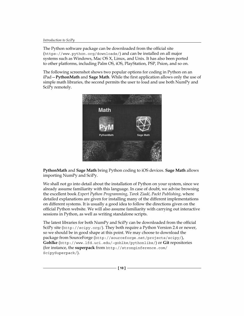
The following screenshot shows two popular options for coding in Python on an iPad—PythonMath and Sage Math. While the fi rst application allows only the use of simple math libraries, the second permits the user to load and use both NumPy and SciPy remotely.

PythonMath and Sage Math bring Python coding to iOS devices. Sage Math allows importing NumPy and SciPy.

We shall not go into detail about the installation of Python on your system, since we already assume familiarity with this language. In case of doubt, we advise browsing the excellent book Expert Python Programming, Tarek Ziadé, Packt Publishing, where detailed explanations are given for installing many of the different implementations on different systems. It is usually a good idea to follow the directions given on the offi cial Python website. We will also assume familiarity with carrying out interactive sessions in Python, as well as writing standalone scripts.

The latest libraries for both NumPy and SciPy can be downloaded from the offi cial SciPy site (http://scipy.org/). They both require a Python Version 2.4 or newer, so we should be in good shape at this point. We may choose to download the package from SourceForge (http://sourceforge.net/projects/scipy/), Gohlke (http://www.lfd.uci.edu/~gohlke/pythonlibs/) or Git repositories (for instance, the superpack from http://stronginference.com/ScipySuperpack/).

Chapter 1

[ 11 ]

It is also possible in some systems to use prepackaged executable bundles that simplify the process, such as the Anaconda (https://store.continuum.io/cshop/anaconda/) or the Enthought (https://www.enthought.com/products/epd/) Python distributions. Here, we will show you how to download and install Scipy on various platforms in the most common cases.

Installing SciPy on Mac OS XWhile installing SciPy on Mac OS X, you must consider some criteria before you install it on your system. This helps in smooth installation of SciPy. The following are the things to be taken care of:

• For instance, in Mac OS X, if MacPorts is installed, the process could not be easier. Open a terminal as superuser, and at the prompt (%), issue the following command:% port search scipy

• This presents a list of all ports that either install SciPy or use SciPy as a requirement. For Python 2.7 we need to install py27-scipy issuing the following command:

% port install py27-scipy

A few minutes later, the libraries are properly installed and ready to use. Note how macports also installs all needed requirements for us (including the NumPy libraries) without any extra effort on our part.

Installing SciPy on Unix/LinuxUnder any other Unix/Linux system, if either no ports are available or if the user prefers to install from the packages downloaded from either SourceForge or Git, it is enough to perform the following steps:

1. Unzip the NumPy and SciPy packages following the recommendation of the offi cial pages. This creates two folders, one for each library.Within a terminal session, change directories to the folder where the NumPy libraries are stored, which contains the setup.py fi le. Find out which Fortran compiler you are using (one of gnu, gnu95, or fcompiler), and at prompt, issue the following command:

% python setup.py build –fcompiler=<compiler>

Introduction to SciPy

[ 12 ]

2. Once built, and on the same folder, issue the installation command. This should be all:

% python setup.py install

Installing SciPy on WindowsYou can install Scipy on Windows in many ways. The following are some recommended ways that you might want to have a look on:

• Under Microsoft Windows, we recommend you install from the binary installers provided by the Anaconda or Enthought Python Distributions. Please, however, be aware of the memory requirements. Alternatively, you can download and install the SciPy stack or the libraries, individually.

• The procedure for the installation of the SciPy libraries is exactly the same, that is, downloading and building before installing under Unix/Linux or downloading and running under Microsoft Windows. Note that different implementations of Python might have different requirements before installing NumPy and SciPy.

Testing the SciPy installationAs you might know, computer systems are not infallible. Accordingly, before starting computing via SciPy, one needs to be sure it is working correctly. To that end, SciPy developers have included a test suit any user of SciPy can execute to be sure the SciPy being used is working fi ne. That way, much debugging time can be saved whenever an error occurs while using any function provided by SciPy.

To run the test suite, at the Python prompt, one can run the following commands:

>>> import scipy

>>> scipy.test()

Downloading the example codeYou can download the example code fi les for all Packt books you have purchased from your account at http://www.packtpub.com. If you purchased this book elsewhere, you can visit http://www.packtpub.com/support and register to have the fi les e-mailed directly to you.

Chapter 1

[ 13 ]

The reader should be aware that the execution of this test will take some time to fi nish. It should end with something like this:

This means that at the basic level, your SciPy installation is fi ne. Eventually, the test could end in the form:

In this case, one needs to revise carefully the errors and the failed tests. A place to get help is the SciPy mailing list (http://mail.scipy.org/pipermail/scipy-user/) to which one could subscribe. We have included a Python script that the reader could use to run these tests that can be found at the companion software for this chapter that comes with the book.

Introduction to SciPy

[ 14 ]

SciPy organizationSciPy is organized as a family of modules. We like to think of each module as a different fi eld of mathematics. And as such, each has its own particular techniques and tools. You can fi nd a list of some of the different modules included in SciPy at http://docs.scipy.org/doc/scipy-0.14.0/reference/py-modindex.html.

Let's use some of its functions to solve a simple problem.

The following table shows the IQ test scores of 31 individuals:

114 100 104 89 102 91 114 114103 105 108 130 120 132 111 128118 119 86 72 111 103 74 112107 103 98 96 112 112 93

A stem plot of the distribution of these 31 scores (refers to the IPython Notebook for this chapter) shows that there are no major departures from normality, and thus we assume the distribution of the scores to be close to normal. Now, estimate the mean IQ score for this population, using a 99 percent confi dence interval.

We start by loading the data into memory, as follows:

>>> import numpy

>>> scores = numpy.array([114, 100, 104, 89, 102, 91, 114, 114, 103, 105, 108, 130, 120, 132, 111, 128, 118, 119, 86, 72, 111, 103, 74, 112, 107, 103, 98, 96, 112, 112, 93])

At this point, if we type dir(scores), hit the return key followed by a dot (.), and press the tab key ;the system lists all possible methods inherited by the data from the NumPy library, as it is customary in Python. Technically, we could go ahead and compute the required mean, xmean, and corresponding confi dence interval according to the formula, xmean ± zcrit * sigma / sqrt(n), where sigma and n are respectively the standard deviation and size of the data, and zcrit is the critical value corresponding to the confi dence (http://en.wikipedia.org/wiki/Confidence_interval). In this case, we could look up a table on any statistics book to obtain a crude approximation to its value, zcrit = 2.576. The remaining values may be computed in our session and properly combined, as follows:

>>> import scipy

>>> xmean = scipy.mean(scores)

>>> sigma = scipy.std(scores)

Chapter 1

[ 15 ]

>>> n = scipy.size(scores)

>>> xmean, xmean - 2.576*sigma /scipy.sqrt(n), \

xmean + 2.576*sigma / scipy.sqrt(n)

The output is shown as follows:

(105.83870967741936, 99.343223715529746, 112.33419563930897)

We have thus computed the estimated mean IQ score (with value 105.83870967741936) and the interval of confi dence (from about 99.34 to approximately 112.33 ). We have done so using purely SciPy-based operations while following a known formula. But instead of making all these computations by hand and looking for critical values on tables, we could just ask SciPy.

Note how the scipy.stats module needs to be loaded before we use any of its functions:

>>> from scipy import stats

>>> result=scipy.stats.bayes_mvs(scores)

The variable result contains the solution to our problem with some additional information. Note that result is a tuple with three elements as the help documentation suggests:

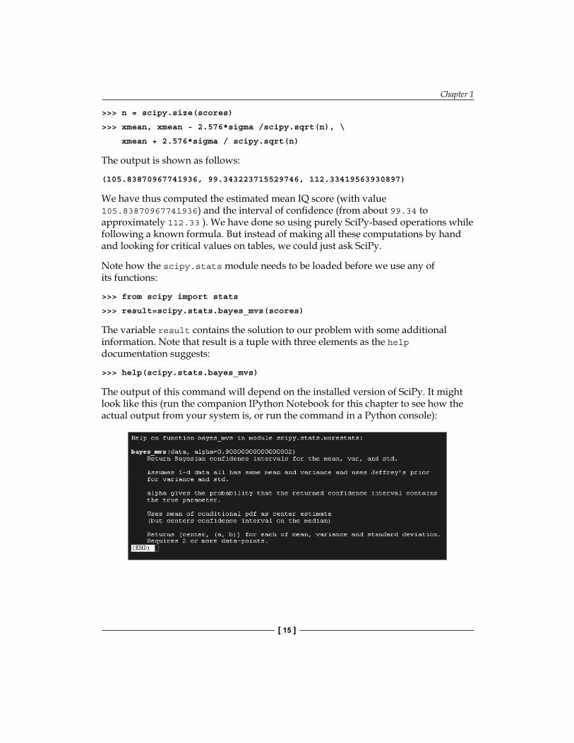
>>> help(scipy.stats.bayes_mvs)

The output of this command will depend on the installed version of SciPy. It might look like this (run the companion IPython Notebook for this chapter to see how the actual output from your system is, or run the command in a Python console):

Introduction to SciPy

[ 16 ]

Our solution is the fi rst element of the tuple result; to see its contents, type:

>>> result[0]

The output is shown as follows:

(105.83870967741936, (101.48825534263035, 110.18916401220837))

Note how this output gives us the same average as before, but a slightly different confi dence interval, due to more accurate computations through SciPy (the output might be different depending on the SciPy version available on your computer).

How to fi nd documentationThere is a wealth of information online, either from the offi cial pages of SciPy (although its reference guides are somehow incomplete, as a work in progress), or from many other contributors that present tutorials on forums, YouTube, or personal sites. Several developers also publish examples of their work with great detail online.

As we previously saw, it is also possible to obtain help from our interactive Python sessions. The libraries NumPy and SciPy make use of docstrings heavily, which makes it simple to request for help for usage and recommendations with the usual Python help system. For example, if in doubt of the usage of the bayes_mvs routine, the user can issue the following command:

>>> import scipy.stats

>>> help(scipy.stats.bayes_mvs)

After executing this command, the system provides the necessary information. Equivalently, both NumPy and SciPy come bundled with their own help system, info. For instance, look at the following command:

>>> import numpy

>>> numpy.info('random')

This will offer a summary of all information parsed from the contents of all docstrings from the NumPy library associated with the given keyword (note it must be quoted). The user may navigate the output scrolling up and down, without the possibility of further interaction.

This is convenient provided we already do know the function we want to use if we are unsure of its usage. But, what should we do if we don't know about the existence of this procedure, and suspect that it may exist? The usual Python way is to invoke the dir() command on a module, which lists all possible attributes.

Chapter 1

[ 17 ]

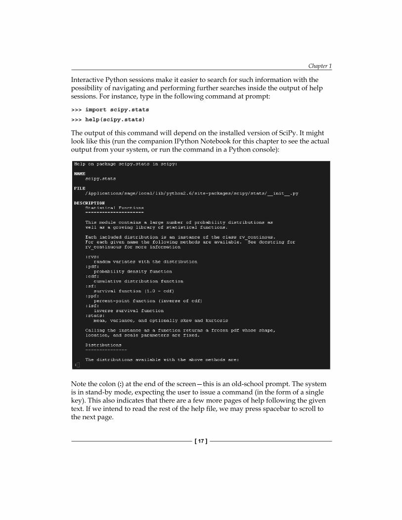
Interactive Python sessions make it easier to search for such information with the possibility of navigating and performing further searches inside the output of help sessions. For instance, type in the following command at prompt:

>>> import scipy.stats

>>> help(scipy.stats)

The output of this command will depend on the installed version of SciPy. It might look like this (run the companion IPython Notebook for this chapter to see the actual output from your system, or run the command in a Python console):

Note the colon (:) at the end of the screen—this is an old-school prompt. The system is in stand-by mode, expecting the user to issue a command (in the form of a single key). This also indicates that there are a few more pages of help following the given text. If we intend to read the rest of the help fi le, we may press spacebar to scroll to the next page.

Introduction to SciPy

[ 18 ]

In this way, we can visit the following manual pages on this topic. It is also possible to navigate the manual pages scrolling one line of text at a time using the up and down arrow keys. When we are ready to quit the help session, we simply press (the keyboard letter) Q.

It is also possible to search the help contents for a given string. In that case, at the prompt, we press the (/) slash key. The prompt changes from a colon into a slash, and we proceed to input the keyword we would like to search for.

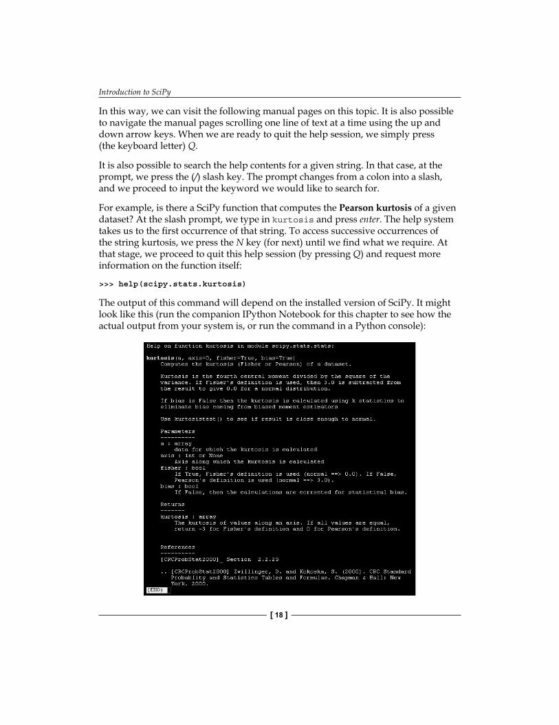
For example, is there a SciPy function that computes the Pearson kurtosis of a given dataset? At the slash prompt, we type in kurtosis and press enter. The help system takes us to the fi rst occurrence of that string. To access successive occurrences of the string kurtosis, we press the N key (for next) until we fi nd what we require. At that stage, we proceed to quit this help session (by pressing Q) and request more information on the function itself:

>>> help(scipy.stats.kurtosis)

The output of this command will depend on the installed version of SciPy. It might look like this (run the companion IPython Notebook for this chapter to see how the actual output from your system is, or run the command in a Python console):

Chapter 1

[ 19 ]

Scientifi c visualizationAt this point, we would like to introduce you to another resource that we will be using to generate graphs, namely the matplotlib libraries. It may be downloaded from its offi cial web page, http://matplotlib.org/, and installed following the standard Python commands. There is a good online documentation in the offi cial web page, and we encourage the reader to dig deeper than the few commands that we will use in this book. For instance, the excellent monograph Matplotlib for Python Developers, Sandro Tosi, Packt Publishing, provides all that we would need and more. Other plotting libraries are available (commercial or otherwise that aim to very different and specifi c applications. The degree of sophistication and ease of use of matplotlib makes it one of the best options to generate graphics in scientifi c computing.

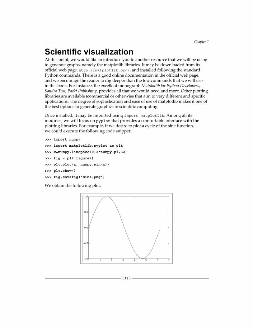
Once installed, it may be imported using import matplotlib. Among all its modules, we will focus on pyplot that provides a comfortable interface with the plotting libraries. For example, if we desire to plot a cycle of the sine function, we could execute the following code snippet:

>>> import numpy

>>> import matplotlib.pyplot as plt

>>> x=numpy.linspace(0,2*numpy.pi,32)

>>> fig = plt.figure()

>>> plt.plot(x, numpy.sin(x))

>>> plt.show()

>>> fig.savefig('sine.png')

We obtain the following plot:

-1.0

1.0

0.5

0.0

-0.5

0 1 2 3 4 5 6 7

Introduction to SciPy

[ 20 ]

Let us explain each command from the previous session. The fi rst two commands are used to import numpy and matplotlib.pyplot as usual. We defi ne an array x of 32 uniformly spaced fl oating point values from 0 to 2π, and defi ne y to be the array containing the sine of the values from x. The command fi gure creates space in the memory to store the subsequent plots and puts in place an object of the matplotlib.figure.Figure form. The plt.plot(x, numpy.sin(x)) command creates an object of the matplotlib.lines.Line2D form containing data with the plot of x against numpy.sin(x) together with a set of axes attached to it and labeled according to the ranges of the variables. This object is stored in the previous Figure object and is displayed on the screen via the plt.show()command. The last command in the session, fig.savefig(), saves the Figure object to whatever valid image format we desire (in this case, a Portable Network Graphics (PNG) image). From now on, in any code that deals with matplotlib commands, we will leave the option of showing/saving open.

There are, of course, commands that control the style of axes, aspect ratio between axes, labeling, colors, legends, the possibility of managing several fi gures at the same time (subplots), and many more features to display all sorts of data. We will be discovering these as we progress with examples throughout the book.

How to open IPython NotebooksThis book comes with a set of IPython Notebooks that will help you interactively test and modify or adapt to your needs to the code snippets shown in each chapter of the book. We should warn, however, that these IPython Notebooks will make sense only if read along side the book.

In this regard, this book assumes familiarity with Python and some of its development environment as the IPython Notebook. Consequently, we will only refer to the documentation on the offi cial website for IPython Notebook (http://ipython.org/notebook.html). You can fi nd additional help at (http://ipython.org/ipython-doc/stable/notebook/index.html). Note that IPython Notebook is also available through Wakari (https://wakari.io/), as a standalone or part of the Anaconda package, or by Enthought. If you're new to IPython Notebook, get started by looking at the example collection and reading the documentation.

To use the fi les for this book, open a terminal and go to the directory where the fi le you want to open is stored (it should have the form filename.ipynb). At the command line, in that terminal, type:

ipython notebook filename.ipynb

Chapter 1

[ 21 ]

After hitting the enter key, the fi le should be displayed in the default web browser. In case that does not happen, please note that the IPython Notebook is offi cially supported on the browsers Chrome, Safari, and Firefox. For additional details refers to the Browser Compatibility section on the documentation currently at http://ipython.org/ipython-doc/stable/install/install.html.

Once the .ipynb fi le has been opened, press and hold the shift key and hit enter to start executing the notebook cell by cell. Another way to execute the notebook cell by cell is via the player icon on the menu near the left of the cell labeled as markdown. Alternatively, from the Cell menu (on the top of the browser) you could choose among several options to execute the contents of the notebook.

To leave the notebook you could choose Close and halt, from the File menu on top of the browser below the label Notebook. Options to save the notebook can also be found under the File menu. To completely close the notebook browser you need to hit the keys ctrl and C simultaneously on the terminal where the notebook was started and follow the instructions after that.

SummaryIn this chapter, you have learned the benefi ts of using the combination of Python, NumPy, SciPy, and matplotlib as a programming environment for any scientifi c endeavor that requires mathematics; in particular, anything related to numerical computations. You have explored the environment, learned how to download, install, and test the required libraries, used them for some quick computations, and fi gured out a few good ways to search for help.

In Chapter 2, Working with the NumPy Array As a First Step to SciPy, we will guide you through basic object creation in SciPy, including the best methods to manipulate data, or obtain information from it.

Where to buy this book You can buy Learning SciPy for Numerical and Scientific Computing Second Edition from the Packt Publishing website. Alternatively, you can buy the book from Amazon, BN.com, Computer Manuals and most internet book retailers.

Click here for ordering and shipping details.

www.PacktPub.com

Stay Connected:

Get more information Learning SciPy for Numerical and Scientific Computing Second Edition