The 4th International Conference on Field and Service Robotics, July 14–16, 2003

Learning Predictions of the Load-Bearing Surface for AutonomousRough-Terrain Navigation in Vegetation

Carl Wellington Anthony (Tony) Stentz

Robotics Institute Robotics InstituteCarnegie Mellon University Carnegie Mellon UniversityPittsburgh, PA 15201 USA Pittsburgh, PA 15201 USA

cwellin@ri.cmu.edu axs@ri.cmu.edu

Abstract

Current methods for off-road navigation using vehicleand terrain models to predict future vehicle response arelimited by the accuracy of the models they use and can suf-fer if the world is unknown or if conditions change and themodels become inaccurate. In this paper, an adaptive ap-proach is presented that closes the loop around the vehiclepredictions. This approach is applied to an autonomousvehicle driving through unknown terrain with varied vege-tation. Features are extracted from range points from for-ward looking sensors. These features are used by a locallyweighted learning module to predict the load-bearing sur-face, which is often hidden by vegetation. The true surfaceis then found when the vehicle drives over that area, andthis feedback is used to improve the model. Results usingreal data show improved predictions of the load-bearingsurface and successful adaptation to changing conditions.

1 Introduction and Related WorkAutomated vehicles that can safely operate in rough ter-

rain hold the promise of higher productivity and efficiencyby reducing the need for skilled operators, increased safetyby removing people from dangerous environments, and animproved ability to explore difficult domains on earth andother planets. Even if a vehicle is not fully autonomous,there are benefits from having a vehicle that can reasonabout its environment to keep itself safe. Such systems canbe used in safeguarded teleoperation or as an additionalsafety system for human operated vehicles.

To safely perform tasks in unstructured environments,an automated vehicle must be able to recognize terrain in-teractions that could cause damage to the vehicle. Thisis a difficult problem because there are complex dynamicinteractions between the vehicle and the terrain that are of-ten unknown and can change over time, vegetation is com-

pressible which prevents a purely geometric interpretationof the world, there are catastrophic states such as rolloverthat must be avoided, and there is uncertainty in everything.In agricultural applications, much about the environment isknown, but unexpected changes can occur due to weather,and the vehicle is often required to drive through vegetationthat changes during the year. In more general off-road ex-ploration tasks, driving through vegetated areas may savetime or provide the only possible route to a goal destina-tion, and the terrain is often unknown to the vehicle.

Many researchers have approached the rough terrainnavigation problem by creating terrain representationsfrom sensor information and then using a vehicle modelto make predictions of the future vehicle trajectory to de-termine safe control actions [1, 2, 3, 4]. These techniqueshave been successful on rolling terrain with discrete ob-stacles and have shown promise in more cluttered environ-ments, but handling vegetation remains a challenge.

Navigation in vegetation is difficult because the rangepoints from stereo cameras or a laser range-finder do notgenerally give the load-bearing surface. Classification ofvegetation and solid substances can be useful for this task,but it is not sufficient. A grassy area on a steep slope maybe dangerous to drive on whereas the same grass on a flatarea could be easily traversable. Researchers have mod-eled the statistics of laser data in grass to find hard ob-jects [5], assigned spring models to different terrain classesto determine traversability using a simple dynamic analy-sis [4], and kept track of the ratio of laser hits to laser pass-throughs to determine the ground surface in vegetation [3].

The above methods all rely on various forms of vehicleand terrain models. These models are difficult to construct,hard to tune, and if the terrain is unknown or changing, themodels can become inaccurate and the predictions will bewrong. Incorrect predictions may lead to poor decisionsand unsafe vehicle behavior. In this work, we investigatemodel learning methods to mitigate this problem.

Other researchers have investigated the use of parameteridentification techniques with soil models to estimate soilparameters on-line from sensor data [6, 7], but these meth-ods only determine the terrain that the vehicle is currentlytraversing. We are interested in taking this a step furtherand closing the loop around the vehicle predictions them-selves by learning a better mapping from forward lookingsensor data to future vehicle state. This allows the vehi-cle to use its experience from interacting with the terrain toadapt to changing conditions and improve its performanceautonomously.

Our vehicle test platform is described in section 2 andour model-based approach to safeguarding in rough terrainis given in section 3. Section 4 explains the general ap-proach of learning vehicle predictions and then describeshow this is used to find the load-bearing surface in veg-etation. Experimental results are given in section 5 andconclusions and future work are given in section 6.

2 Vehicle Platform and Terrain MappingOur project team [8] has automated a John Deere 6410

tractor (see figure 1). This vehicle has a rich set of sen-sors, including a differential GPS unit, a 3-axis fiber opticvertical gyro, a doppler radar ground speed sensor, a steer-ing angle encoder, four custom wheel encoders, a high-resolution stereo pair of digital cameras, and two SICKlaser range-finders (ladar) mounted on custom activelycontrolled scanning mounts. The first ladar on the roofof the vehicle is mounted horizontally and is scanned tocover the area in front of the tractor. The ladar on the frontbumper is mounted vertically and is actively scanned inthe direction the tractor is steering. We are currently ex-perimenting with a near-infrared camera and a millimeter-wave radar unit as well.

The approach described in this work builds maps usingrange points from multiple lasers that are actively scannedwhile the vehicle moves over rough terrain. The trueground surface is then found when the tractor drives overthat area a number of seconds later. To make this pro-cess work, it is important that the scanned ladars are pre-cisely calibrated and registered with each other in the trac-tor frame, the timing of all the various pieces of sensordata is carefully synchronized, and the vehicle has a pre-cise pose estimate. Our system has a 13 state extendedKalman filter with bias compensation and outlier rejectionthat integrates the vehicle sensors described above into anaccurate estimate of the pose of the vehicle at 75Hz. Thispose information is used to tightly register the data fromthe ladars into high quality terrain maps.

The information from the forward looking sensors rep-resents a massive amount of data in its raw form, so someform of data reduction is needed. One simple approach is

Figure 1: Automated tractor test platform.

to create a grid in the world frame and then combine theraw data into summary information such as average heightfor each grid cell. This approach makes it easy to com-bine range information from the two ladars on our vehicleand to combine sensor information over time as the vehicledrives. Figure 3 shows the type of terrain we tested on anda grid representation of this area using the average heightof each cell.

3 Rough Terrain Navigation

The goal of our system is to follow a predefined paththrough rough terrain while keeping the vehicle safe. Pathtracking is performed using a modified form of pure pur-suit [8]. The decision to continue is based on safety thresh-olds on the model predictions for roll, pitch, clearance, andsuspension limits. These quantities are found by building amap of the upcoming terrain and using a vehicle model toforward simulate the expected trajectory on that terrain [2].

If the vehicle is moving relatively slowly and the load-bearing surface of the surrounding terrain can be measured,these quantities can be computed using a simple kinematicanalysis. The trajectory of the vehicle is simulated forwardin time using its current velocity and steering angle. Akinematic model of the vehicle is then placed on the ter-rain map at regular intervals along the predicted trajectory,and the heights of the four wheels are found in order tomake predictions of vehicle roll and pitch. The clearanceunder the vehicle is important for finding body collisionsand high centering hazards. It is found by measuring thedistance from the height of the ground in each cell underthe vehicle to the plane of the bottom of the vehicle. Ourvehicle has a simple front rocker suspension, so checkingthe suspension limits involves calculating the roll of thefront axle and comparing it to the roll of the rear axle. Forsmooth terrain with solid obstacles, this approach workswell because accurate predictions of the load bearing sur-

face can be found by simply averaging the height of therange points in the terrain map.

If there is vegetation, finding the load-bearing surfacecan be difficult because many laser range points hit vari-ous places on the vegetation instead of the ground. Sim-ply averaging the points in a grid cell performs poorly inthis case. One possible solution is to use the lowest pointin each grid cell instead. This correctly ignores the rangepoints that hit vegetation, but because there is inevitablenoise in the range points (especially at long distances), thisresults in the lowest outlier in the noise distribution beingchosen, thus underestimating the true ground height.

4 Learning Vehicle PredictionsTo overcome the difficulties associated with creating ve-

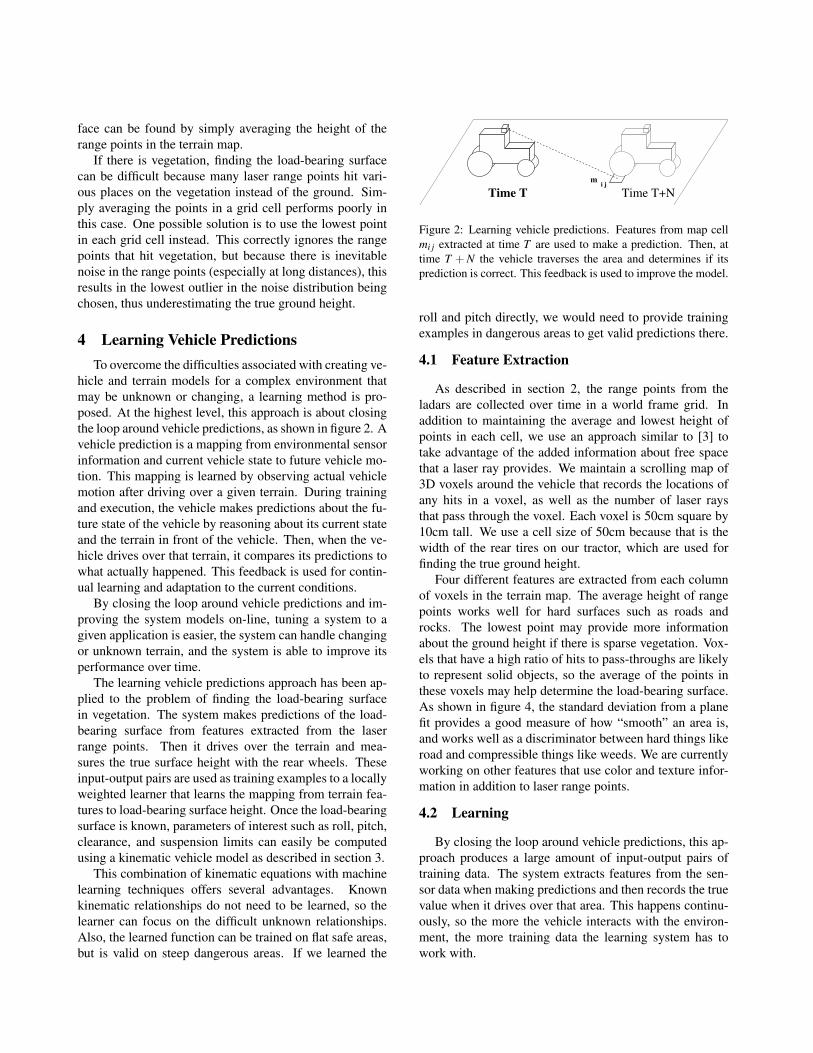
hicle and terrain models for a complex environment thatmay be unknown or changing, a learning method is pro-posed. At the highest level, this approach is about closingthe loop around vehicle predictions, as shown in figure 2. Avehicle prediction is a mapping from environmental sensorinformation and current vehicle state to future vehicle mo-tion. This mapping is learned by observing actual vehiclemotion after driving over a given terrain. During trainingand execution, the vehicle makes predictions about the fu-ture state of the vehicle by reasoning about its current stateand the terrain in front of the vehicle. Then, when the ve-hicle drives over that terrain, it compares its predictions towhat actually happened. This feedback is used for contin-ual learning and adaptation to the current conditions.

By closing the loop around vehicle predictions and im-proving the system models on-line, tuning a system to agiven application is easier, the system can handle changingor unknown terrain, and the system is able to improve itsperformance over time.

The learning vehicle predictions approach has been ap-plied to the problem of finding the load-bearing surfacein vegetation. The system makes predictions of the load-bearing surface from features extracted from the laserrange points. Then it drives over the terrain and mea-sures the true surface height with the rear wheels. Theseinput-output pairs are used as training examples to a locallyweighted learner that learns the mapping from terrain fea-tures to load-bearing surface height. Once the load-bearingsurface is known, parameters of interest such as roll, pitch,clearance, and suspension limits can easily be computedusing a kinematic vehicle model as described in section 3.

This combination of kinematic equations with machinelearning techniques offers several advantages. Knownkinematic relationships do not need to be learned, so thelearner can focus on the difficult unknown relationships.Also, the learned function can be trained on flat safe areas,but is valid on steep dangerous areas. If we learned the

Time T+NTime Tm i j

Figure 2: Learning vehicle predictions. Features from map cellmi j extracted at time T are used to make a prediction. Then, attime T + N the vehicle traverses the area and determines if itsprediction is correct. This feedback is used to improve the model.

roll and pitch directly, we would need to provide trainingexamples in dangerous areas to get valid predictions there.

4.1 Feature Extraction

As described in section 2, the range points from theladars are collected over time in a world frame grid. Inaddition to maintaining the average and lowest height ofpoints in each cell, we use an approach similar to [3] totake advantage of the added information about free spacethat a laser ray provides. We maintain a scrolling map of3D voxels around the vehicle that records the locations ofany hits in a voxel, as well as the number of laser raysthat pass through the voxel. Each voxel is 50cm square by10cm tall. We use a cell size of 50cm because that is thewidth of the rear tires on our tractor, which are used forfinding the true ground height.

Four different features are extracted from each columnof voxels in the terrain map. The average height of rangepoints works well for hard surfaces such as roads androcks. The lowest point may provide more informationabout the ground height if there is sparse vegetation. Vox-els that have a high ratio of hits to pass-throughs are likelyto represent solid objects, so the average of the points inthese voxels may help determine the load-bearing surface.As shown in figure 4, the standard deviation from a planefit provides a good measure of how “smooth” an area is,and works well as a discriminator between hard things likeroad and compressible things like weeds. We are currentlyworking on other features that use color and texture infor-mation in addition to laser range points.

4.2 Learning

By closing the loop around vehicle predictions, this ap-proach produces a large amount of input-output pairs oftraining data. The system extracts features from the sen-sor data when making predictions and then records the truevalue when it drives over that area. This happens continu-ously, so the more the vehicle interacts with the environ-ment, the more training data the learning system has towork with.

Figure 3: Top: Test area showing dirt roads and vegetation.Bottom: Map of test area using average height.

The mapping between the laser point features and thetrue ground height is unknown and potentially complex,so we use a general purpose function approximator forthis task. Among the many possibilities, locally weightedlearning [9] was chosen because it can accurately fit com-plex functions, it produces confidence estimates on its pre-dictions, and there are online versions available.

A common form of locally weighted learning is locallyweighted regression (LWR). Training with this algorithmsimply involves inserting input-output pairs into memory.Then, when a new prediction is requested, the points inmemory are weighted by a kernel function of the distanceto the new query point, and a local multi-dimensional lin-ear regression is performed on these weighted data pointsto produce a prediction. For good results, the kernel widthmust be chosen properly so that the resulting function doesnot over-fit or over-smooth the data. We use global leave-one-out cross validation to find the kernel width.

Standard statistical techniques for computing predic-tion bounds have been adapted to be used with this algo-rithm [10]. The size of the prediction bound depends bothon the density of data points in the area, and on the noise inthe outputs of nearby data points that cannot be explainedby the model. The prediction bounds assume that the lin-ear model structure is correct and the noise is zero-meanGaussian. These assumptions can rarely be verified, butbecause they only have to be satisfied locally, the predic-tion bounds still give useful information in practice about

Standard deviation from plane fit (cm)

50 100 150

50

100

150

200

250

300

350

4000

5

10

15

20

Figure 4: The standard deviation from a plane fit is found foreach cell in the terrain map to discriminate between hard thingslike road and compressible things like weeds.

the confidence in the prediction.Locally weighted learning stores all of its training data,

so predictions take longer to compute as more training datais collected. This is not practical for systems such as oursthat receive a continuous stream of data. Schaal [11] hasdescribed an on-line incremental version of LWR calledreceptive field weighted regression (RFWR). Instead ofpostponing all computations until a new prediction is re-quested, RFWR incrementally builds a set of receptivefields, each of which has a local regression model that isincrementally updated. The data points are then discarded,and predictions are made from a combination of nearby re-ceptive fields. A forgetting factor is used to slowly discountold experience as it is replaced with new data.

5 Experimental Results

A set of experiments were performed to test the ca-pabilities of this system. The first experiment shows theimproved performance of the learned predictions and theusefulness of prediction bounds. The second experimentshows the system’s ability to adapt to a change in the envi-ronment.

Although the analysis for the following experimentswas performed off-line, the data used was collected in re-alistic conditions at the test site shown in figure 3. We col-lected approximately 25 minutes of data traveling on dirtroads and driving through varied vegetation often over ameter tall. Traveling at a speed of 1 m/s, we logged input-output pairs of laser features and corresponding rear wheelheight at a rate of 4 examples per second, giving a total of5700 data points. The data from the section shown in fig-ure 3 was used as the test set, and the remaining 75% ofthe data was used for training.

150 200 250 300−20

0

20

40

60

80

Distance along path (m)Dev

iatio

n fro

m g

roun

d he

ight

(cm

)

Right wheel height predictions

Ave PtLearnedLow Pt

150 200 250 3000

10

20

30

40

Distance along path (m)

Pre

d B

ound

(cm

)

Road Road Road

95% Prediction bound

Figure 5: Top: Height prediction deviations for right wheel(should be zero). Average point has trouble in grass, lowest pointunderestimates, learned predictions do better. Bottom: Learnerproduces prediction bounds on its estimate that are lower for thesmooth road areas and high for some of the tall vegetation.

5.1 Performance Improvement

The locally weighted regression technique described insection 4 was used to find a model for the training datadescribed above. Leave-one-out cross validation was usedto choose the kernel bandwidth. Figure 5 shows heightprediction results for a section of the test set. The topgraph shows the errors in predicted heights using the av-erage height, the lowest point, and the learned result usingall the features described in section 4.1. It can be seenthat using the average point does quite poorly in vegetationand using the lowest point can result in outlier points be-ing chosen. This especially occurs on roads where manylaser points are recorded at long range (10m), resulting inhigher uncertainty. The learned result has smaller errorsthan either of these because it is able to combine the differ-ent features in an appropriate way. The lower graph showsthe 95% prediction intervals produced by LWR. The threetimes that the vehicle drives on the road are clearly shownby the tighter prediction bounds, and the learner has verylittle confidence in its predictions for some of the pointsin deep vegetation. These bounds are important becausethey could be used to modify the behavior of the vehicle.On simple terrain such as roads where the learner is con-fident, the vehicle could drive faster or attempt more ex-treme angles. In difficult terrain with tall vegetation wherethe learner has low confidence, the vehicle could approachthe area with caution or avoid it completely.

Figure 6 shows that combining all the features using

−20

−15

−10

−5

0

5

10

15

20

Dev

iatio

n fro

m tr

ue g

roun

d he

ight

(cm

)

Technique

Results comparison

AveHeight

Ave HeightSolid Voxels

LowestHeight

Global LinearRegression

LWR

Mean and 1−sigma deviation from true ground height

Figure 6: Comparison of the performance of the different featuresalong with global and local regression on the test set.

0 1 2 3 4 5 6 7 8−50

0

50

Prediction distance in front of the tractor (m)

Dev

iatio

n fro

m tr

ue g

roun

d he

ight

(cm

)

Error for different prediction distances

Mean 95% prediction bound from learnerMean and 2−sigma (95%) level of prediction error

Figure 7: Error of predictions on the test set at different distancesusing LWR. The prediction bounds from the learner are similar tothe actual prediction errors.

global or local regression performs better than using anyof the features individually. LWR can represent the smallnon-linearities in this problem and performs slightly betterthan global linear regression. More importantly, LWR pro-duces local prediction bounds that reflect the confidencein the prediction at that particular location in the featurespace, allowing the system to be cautious in areas it hasn’texperienced before.

The height predictions in figures 5 and 6 use all the laserpoints that are collected for a given patch of terrain. Inpractice, this would only happen if the system made pre-dictions of future vehicle motion just in front of its currentlocation. This is not useful if the vehicle cannot react in thisdistance. Figure 7 shows the effect of making predictionsfurther ahead of the vehicle. The plot shows that the spreadof the prediction errors increases when the predictions aremade farther into the future. The figure also shows themean 95% prediction bound the learner produces for dif-

0 500 1000 1500 2000 25000

2

4

6

8

10

12

14

16

18

Training samples

Mea

n ab

solu

te te

st e

rror

(cm

)

Learning during a change in the environment

Site A

Site B

Figure 8: After learning a model for Site A using RFWR, thesystem is transported to Site B. The error rises initially, but thenthe system adapts to the new environment.

ferent prediction distances. This curve is similar to the 2σ(95%) level on the error, again showing the usefulness ofthe prediction bounds.

5.2 Adapting to Environmental Change

The above tests were performed in batch mode usinglocally weighted linear regression. In this experiment, theon-line receptive field weighted regression algorithm wasused to test the system’s ability to adapt to a changing en-vironment. We collected more data in another test site thathad dense vegetation approximately 0.75m high. This datawas split into a training and test set. The training data waspresented to the RFWR learning algorithm, and the predic-tion error on the test set was periodically computed.

Figure 8 shows the algorithm learning the characteris-tics of this site and reducing prediction error on the testset. Then, starting with sample 1000, the system was pre-sented data used in the previous experiments. After beingtrained in the first site with dense vegetation, the algorithmdid poorly in the new site with roads and more varied veg-etation. However, the learner quickly adapted to the newenvironment and ended up with a prediction error similarto the batch mode version of LWR on the test set. Thisexperiment shows the importance of using an adaptive ap-proach to be able to handle a changing environment.

6 Conclusions and Future Work

We have described the general approach of learning ve-hicle predictions for local navigation, and we have appliedthe technique to the problem of finding the load-bearingsurface in vegetation. The locally weighted learning so-lution to this problem performed better than using a par-ticular feature or performing global linear regression. An-

other benefit of this technique is that it produces predic-tion bounds on its estimate, and these were shown to befairly accurate. Finally, the ability of the system to adaptto changing environmental conditions was shown.

Future work in this area will include an investigationinto other features such as color and texture from cameradata, and the use of the prediction bounds for better vehiclecontrol. We will also investigate whether the technique oflearning vehicle predictions can be applied to other rough-terrain navigation problems such as finding terrain frictioncharacteristics or dynamic vehicle response.

Acknowledgments

This work has been supported by John Deere under con-tract number 476169. The authors would like to thankJeff Schneider for the use of his Vizier code for locallyweighted learning, and Stefan Schaal for the use of his codefor incremental locally weighted learning.

References[1] M. Daily, J. Harris, D. Keirsey, D. Olin, D. Payton, K. Reiser,

J. Rosenblatt, D. Tseng, and V. Wong, “Autonomous cross-countrynavigation with the ALV,” in IEEE Int. Conf. on Robotics and Au-tomation (ICRA 88), vol. 2, pp. 718–726, April 1988.

[2] A. Kelly and A. Stentz, “Rough terrain autonomous mobility -part 2: An active vision, predictive control approach,” AutonomousRobots, vol. 5, pp. 163–198, May 1998.

[3] A. Lacaze, K. Murphy, and M. DelGiorno, “Autonomous mobilityfor the Demo III experimental unmanned vehicles,” in Assoc. forUnmanned Vehicle Systems Int. Conf. on Unmanned Vehicles (AU-VSI 02), July 2002.

[4] A. Talukder, R. Manduchi, R. Castano, K. Owens, L. Matthies,A. Castano, and R. Hogg, “Autonomous terrain characterisation andmodelling for dynamic control of unmanned vehicles,” in IEEE/RSJInt. Conf. on Intelligent Robots and Systems (IROS 02), pp. 708–713, October 2002.

[5] J. Macedo, R. Manduchi, and L. Matthies, “Ladar-based discrimi-nation of grass from obstacles for autonomous navigation,” in Int.Symposium on Experimental Robotics (ISER 00), December 2000.

[6] A. T. Le, D. Rye, and H. Durrant-Whyte, “Estimation of track-soilinteractions for autonomous tracked vehicles,” in IEEE Int. Conf. onRobotics and Automation (ICRA 97), vol. 2, pp. 1388–1393, April1997.

[7] K. Iagnemma, H. Shibly, and S. Dubowsky, “On-line terrain param-eter estimation for planetary rovers,” in IEEE Int. Conf. on Roboticsand Automation (ICRA 02), May 2002.

[8] A. Stentz, C. Dima, C. Wellington, H. Herman, and D. Stager,“A system for semi-autonomous tractor operations,” AutonomousRobots, vol. 13, pp. 87–104, July 2002.

[9] C. Atkeson, A. Moore, and S. Schaal, “Locally weighted learning,”AI Review, vol. 11, pp. 11–73, April 1997.

[10] S. Schaal and C. G. Atkeson, “Assessing the quality of learned lo-cal models,” in Advances in Neural Information Processing Systems(NIPS 94), pp. 160–167, 1994.

[11] S. Schaal and C. G. Atkeson, “Constructive incremental learn-ing from only local information,” in Neural Computation, vol. 10,pp. 147–184, 1998.