IEEE TRANSACTIONS ON JOURNAL NAME, MANUSCRIPT ID 1

Learning Optimized Local Difference Binaries for

Scalable Augmented Reality on Mobile Devices Xin Yang, Member, IEEE. Kwang-Ting (Tim) Cheng, Fellow, IEEE

Abstract—The efficiency, robustness and distinctiveness of a feature descriptor are critical to the user experience and

scalability of a mobile Augmented Reality (AR) system. However, existing descriptors are either too computationally expensive

to achieve real-time performance on a mobile device such as a smartphone or tablet, or not sufficiently robust and distinctive to

identify correct matches from a large database. As a result, current mobile AR systems still only have limited capabilities, which

greatly restrict their deployment in practice. In this paper, we propose a highly efficient, robust and distinctive binary descriptor,

called Learning-based Local Difference Binary (LLDB). LLDB directly computes a binary string for an image patch using simple

intensity and gradient difference tests on pairwise grid cells within the patch. To select an optimized set of grid cell pairs, we

densely sample grid cells from an image patch and then leverage a modified AdaBoost algorithm to automatically extract a

small set of critical ones with the goal of maximizing the Hamming distance between mismatches while minimizing it between

matches. Experimental results demonstrate that LLDB is extremely fast to compute and to match against a large database due

to its high robustness and distinctiveness. Compared to the state-of-the-art binary descriptors, primarily designed for speed,

LLDB has similar efficiency for descriptor construction, while achieving a greater accuracy and faster matching speed when

matching over a large database with 2.3M descriptors on mobile devices.

Index Terms—Scalable augmented reality, binary descriptor, AdaBoost learning, mobile devices

—————————— ——————————

1 INTRODUCTION

scalable Mobile Augmented Reality (MAR) system that is able to track objects, recognized from a large

database, can facilitate a wide range of applications, such as augmenting an entire book with digital interactions or linking city-wide movie posters or leaflets with multimedia trailers and advisements.

Several MAR systems [21, 22, 23, 24, 25, 26] have been proposed recently, such as Wagner et al.’s pose tracking [21, 22, 23], Klein and Murray’s parallel tracking and map-ping [13] and Ta et al.’s SURFTrac [25]. Despite of their suc-cess in real-time tracking, the scalability of these MAR sys-tems remains limited. In practice, they can only manage a limited number of objects, which greatly restricts their large-scale deployment.

One of the major bottlenecks of today’s MAR systems is the high complexity of computing, matching and storing feature point descriptors used for recognition and tracking. Most existing MAR systems rely on high-dimensional real-valued descriptors, e.g. SIFT [2] and SURF [1], which are too costly for mobile devices with limited computational and memory resources. As a result, most systems can only

afford a small dataset for recognition and tracking. Lightweight binary descriptors are very efficient to

compute, to store and to match by computing the Ham-ming distance between descriptors (i.e. via XOR and bit count operations), attractive options for MAR. Binary Ro-bust Independent Element Feature (BRIEF) [3], the Ori-ented Fast and Rotated BRIEF (ORB) [4], and Fast Retina Keypoint (FREAK) [6] are examples of such binary fea-tures. The common idea behind these features is to direct-ly generate a binary string by comparing intensities be-tween pairs of pixels with in an image patch.

While efficient, existing binary descriptors utilize only average intensities. In addition, they sparsely sample a very small number of pixels and rely on ad hoc schemes to select pixel pairs, cursorily discarding a large portion of available information. These designs greatly limit the dis-tinctiveness of existing binary descriptors. For example, they might fail to distinguish patches of different gradient changes (see Figures 1 (a)-(b)) or with sparse textures (see Figures 1 (c)-(d)). Lack of distinctiveness leads to many false matches when matching against a large database. The existence of false matches demands expensive post-verification methods (e.g. RANdom Sample Consensus (RANSAC) [33] or PROgressive Sample Consensus (PRO-SAC) [32]) for validating matching consensus and more false matches will incur longer runtime for this expensive process. Therefore, using a binary descriptor without suffi-cient distinctiveness could actually increase the overall runtime and limit the scalability of an MAR system.

In this paper we present a new binary descriptor, called Learning-based Local Difference Binary (LLDB), based on our previous work Local Difference Binary (LDB) [7]. Compared to LDB and other existing binary descriptors,

xxxx-xxxx/0x/$xx.00 © 200x IEEE Published by the IEEE Computer Society

————————————————

X. Yang is with the Electrical Computer Engineering Department, Univer-sity of California, Santa Barbara, CA, 93106, USA. E-mail: xinyang@ umail.ucsb.edu.

K. T. Cheng is with the Electrical Computer Engineering Department, University of California, Santa Barbara, CA, 93106, USA. E-mail: tim-cheng@ ece.ucsb.edu. ***Please provide a complete mailing address for each author, as this is the address the 10 complimentary reprints of your paper will be sent

Please note that all acknowledgments should be placed at the end of the paper, before the bibliography (note that corresponding authorship is not noted in affiliation box, but in acknowledgment section).

A

2 IEEE TRANSACTIONS ON JOURNAL NAME, MANUSCRIPT ID

LLDB is more distinctive and robust, thus it can effectively identify correct matches from a large database with fewer verifications, yielding high efficiency in matching. The dis-tinctiveness and robustness of LLDB are achieved through 3 steps. First, LLDB captures the internal patterns of each image patch through a set of binary tests, each of which compares the average intensities and first-order gradients of a pair of image grid cells within the patch. The average intensity and gradients capture both DC and AC compo-nents of a patch, thus they provide a more distinctive basis for binary description. Second, in comparison with existing binary descriptors, LLDB applies a much denser sampling pattern on an image patch, which offers a much richer source of distinctive features. Third, instead of relying on ad hoc schemes used in existing binary descriptors, LLDB uses a modified AdaBoost algorithm for selection of critical pairs of grid cells. The modified AdaBoost targets the fun-damental goal of ideal binary descriptors: minimizing dis-tances between matches while maximizing them between mismatches. Computing LLDB descriptors is extremely fast. Utilizing integral images, the average intensity and first-order gradients of each grid cell can be calculated us-ing only 4~8 add/subtract operations and a multiply oper-ation with the reciprocal of the size of the grid cell.

Our experimental results show that the discriminative ability and robustness of LLDB outperform the state-of-the-art binary descriptors LDB, ORB, BRISK and FREAK, while their computational efficiency is about the same. The per-formance of LLDB is demonstrated via a recognition task with 228 objects and patch tracking on a Motorola Xoom1 tablet. Results show that LLDB is much faster to match and track than its competitors, while achieving a greater accu-racy.

The rest of the paper is organized as follows: Sec. 2 re-views the related work. Sec. 3 presents details of the pro-posed descriptor. In Sec. 4, we evaluate the performance of LLDB for scalable matching and pairwise image matching. Sec. 5 provides experimental results on mobile devices for speed, robustness and discriminative power evaluation. Sec. 6 concludes the paper.

2 RELATED WORK

In this section, we review state-of-the-art MAR systems based on visual features, lightweight binary descriptors and learning image descriptors.

2.1 Visual-Feature-Based MAR Systems

With the proliferation of mobile devices equipped with low-cost high-quality cameras, there have been several emerging MAR systems based on visual recognition and tracking [21, 22, 23, 24, 25, 26]. In such a system, an image frame, captured by a mobile camera, is first described us-ing a set of local feature descriptors, based on which objects in the frame are recognized. Periodic recognition results are bridged by tracking the recognized contents.

Most recent research efforts focused on improving the tracking speed for MAR. Wagner et al. made significant advancement in pose tracking [21, 22, 23] to meet tight real-

time constraints. Klein and Murray [24] implemented par-allel tracking and mapping on a mobile phone. Ta et al. [25] improved the speed by tracking SURF features in con-strained locations. However, none of these efforts ad-dressed the scalability of MAR. High-dimensional and real-valued descriptors are used, which are expensive to match and store. As a result, these systems can only handle a lim-ited number of objects.

There are also several works to facilitate real-time recognition over a larger database for AR. For instance, Taylor [28] proposed a high-speed recognition system sup-porting typical video frame rates. Lepetit et al. [29] recasted matching as a classification problem using randomized trees and traded increased memory usage for faster de-scriptor matching. Takacs et al. [26] exploited the temporal coherency between frames and developed a unified real-time tracking and recognition system. Pilet et al. [30] pre-sented an approach based on learning for retrieval and tracking which can handle hundreds of pictures. However, the scalability of their systems were only evaluated on desktop computers and not yet optimized for real-time requirements on handheld devices. Moreover, these sys-tems may require a high memory usage and database re-dundancy. Therefore, for such systems, supporting a larger database with hundreds of images on a handheld device is very challenging.

Due to the limited computing and memory resources in a mobile device, MAR’s scalability must be addressed – for better user experience and for enabling a wider spectrum of applications. Different from previous works, we focus on improving the scalability of MAR under the efficiency constraint. More specifically, we design a new binary de-scriptor which is very fast to compute, compact to store and efficient to match against a large dataset due to its dis-tinctiveness and robustness.

2.2 Lightweight Binary Descriptors

The increasing demand of handling a larger database on mobile devices stimulates the development of light-weight binary descriptors that are efficient to construct, to match and to store. Notable is the BRIEF descriptor [3] which directly generates bit strings by simple binary tests com-paring pixel intensities in a smoothed image patch. The pixel positions are selected randomly according to a Gaussian distribution. A set of efforts are made to further enhance the performance of BRIEF descriptors. Rublee et al. proposed ORB [4] which incorporates image pyramids

Figure 1: Image patches and existing binary descriptors. (a) is a patch of gradually increasing intensity and (b) consists of two homo-

geneous sub-regions. ①, ② and ③ illustrate three exemplar binary

tests for them, which lead to identical binary descriptor values for (a) and (b). (c) and (d) are patches of sparse intensity textures, it is very likely that most binary tests sample pixels in blank regions, yielding non-distinguishing descriptors.

AUTHOR ET AL.: TITLE 3

and orientation operators into BRIEF to achieve scale and rotation invariance. In addition, rather than randomly select pixel pairs, an ad hoc selection scheme is proposed for selecting highly-variant and uncorrelated pixel pairs. Leutenegger et al. [5] suggested sampling pixels according to a circular sampling strategy and then selects short-distant pairs. The resulting descriptor is called BRISK. Alahi et al. [6] further enhanced BRISK by leveraging a sampling strategy which resembles the retinal ganglion cells distribution. However, as described in Sec. 1, these descriptors utilize only intensities of pixels, sparsely sam-pled from an image patch. In addition, their pixel pair se-lection rules are still ad hoc, thus cannot guarantee a satis-factory descriptor to support a wide range of application tasks. As a result, they are not distinctive and robust enough to effectively localized matched patches in large databases. Post-processing for removing false matches is usually required to ensure sufficient recognition accuracy, increasing the total time cost for MAR. In our previous work [7], we proposed LDB which compares pairs of grid cells within a patch, instead of pairs of pixels, to form binary descriptors. Each grid cell is represented by gradi-ents in addition to intensity summations. However, while more distinctive, LDB still lacks a systematic approach for selecting the best set of grid cells. In addition, non-overlapping gridding, employed in their method, inevita-bly incurs spatial quantization errors.

2.3 Learning Image Descriptors

A number of methods are available for learning an opti-mized design. Winder et al. [9] broke up the entire de-scriptor extraction process into a number of building blocks. For each block they tested multiple algorithms and optimized parameters of each algorithm using Powell’s multidimensional direction set method. Different algo-rithm combinations are evaluated using an image match-ing task. The one achieves the best performance is used as the final design. In [10], Winder et al. further extended this work by focusing exclusively on the DAISY spatial config-uration and extensively testing its combination with sever-al most promising algorithms. In [11], Babenko et al. formu-lated local feature matching as a classification problem and applied boosting to learn a set of features for specific tasks. In contrast to these approaches which aim at finding opti-mal design and related parameters for SIFT-like features, we focus on binary descriptors and our goal is to select a small and optimized set of grid cell feature pairs. Our ap-proach is similar to the Boosted Similarity Sensitive Coding (BoostSSC) [38] which relies on AdaBoost to learn a feature description from a family of weak classifiers. BoostSSC method was further extended in [39] to form a more com-pact description. To better adapt the method to the prob-lem of learning a description for intensity patches, the ap-proach in [39] also replaced BoostSSC’s weak classifiers by gradient energy-based weak classifiers [40]. However, cal-culating the gradient energy of an image patch requires expensive operations for computing the dot product be-tween a set of quantized orientations and the gradient ori-entation at every pixel in the patch. Such a requirement would be too costly for real-time applications on a mobile

handheld device. In contrast, we form our weak classifiers based on local difference patterns which are ultra-fast to compute and distinctive as well. In addition, matching based on descriptors learned in [38] and [39] would require computing a weighted hamming distances between de-scriptors. Hence it’s slow to match against a large database. In our approach, we modified the conventional AdaBoost to learn a binary description so that the (unweighted) hamming distance can be used for efficient matching.

3 LLDB: LEARNING BASED LOCAL DIFFERENCE

BINARY

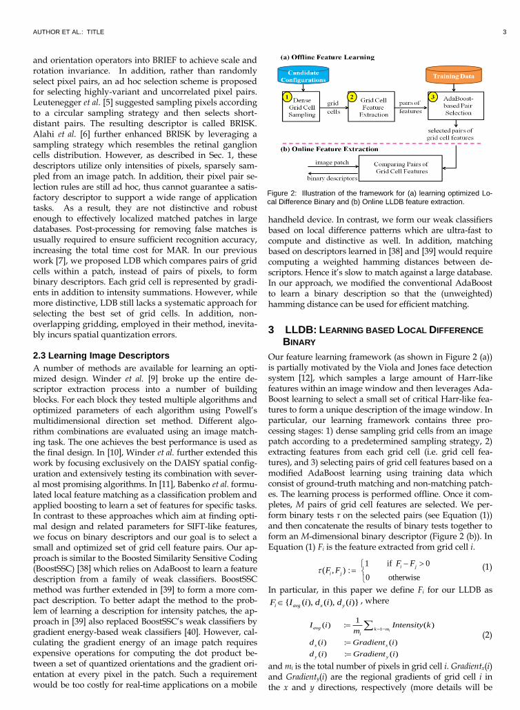
Our feature learning framework (as shown in Figure 2 (a)) is partially motivated by the Viola and Jones face detection system [12], which samples a large amount of Harr-like features within an image window and then leverages Ada-Boost learning to select a small set of critical Harr-like fea-tures to form a unique description of the image window. In particular, our learning framework contains three pro-cessing stages: 1) dense sampling grid cells from an image patch according to a predetermined sampling strategy, 2) extracting features from each grid cell (i.e. grid cell fea-tures), and 3) selecting pairs of grid cell features based on a modified AdaBoost learning using training data which consist of ground-truth matching and non-matching patch-es. The learning process is performed offline. Once it com-pletes, M pairs of grid cell features are selected. We per-form binary tests τ on the selected pairs (see Equation (1)) and then concatenate the results of binary tests together to form an M-dimensional binary descriptor (Figure 2 (b)). In Equation (1) Fi is the feature extracted from grid cell i.

1 if 0 ( , ) :

0 otherwise

i j

i j

F FF F

(1)

In particular, in this paper we define Fi for our LLDB as

{ ( ), ( ), ( )}i avg x yF I i d i d i , where

1~

1( ) : ( )

( ) : ( )

( ) : ( )

iavg k m

i

x x

y y

I i Intensity km

d i Gradient i

d i Gradient i

(2)

and mi is the total number of pixels in grid cell i. Gradientx(i) and Gradienty(i) are the regional gradients of grid cell i in the x and y directions, respectively (more details will be

Figure 2: Illustration of the framework for (a) learning optimized Lo-cal Difference Binary and (b) Online LLDB feature extraction.

4 IEEE TRANSACTIONS ON JOURNAL NAME, MANUSCRIPT ID

presented in Sec. 3.2). In the subsequent sections, we de-scribe each processing stage in detail.

3.1 Dense Gridding Cell Sampling

The sampling strategy (i.e. the distribution of locations and sizes of the sampled grid cells) largely influence the ro-bustness and distinctiveness of the LLDB descriptor. A region with a greater grid cell density and a smaller grid cells encodes more detailed information, thus is more dis-tinctive. On the other hand, a region with a lower density and larger grid cells captures coarser information, and thus is less sensitive to noises.

Several sampling strategies have been explored in exist-ing binary descriptor algorithms [3, 4, 5, 6, 7]. However, these algorithms leverage a low sampling rate. As a result, valuable information is often excluded from the rest of the design pipeline. In contrast, we attempt to retain as much useful information as possible at this stage by densely sampling grid cells according to one of several sampling strategies (which will be discussed in detail lat-er). In our experiment, for each sampling strategy we densely sample 169 grid cells from an image patch which yields 14,196 pairs of pixels, that is 7X more than BRISK, 14.7X more than FREAK, 29X more than LDB, and 54.5X more than BRIEF and ORB. An effective learning algo-rithm is then employed in a successive stage to select a small subset and exclude a vast majority of these pairs to achieve high fidelity.

In this paper, we experimented with six promising strategies which combine three location distributions with either fixed or varying grid cell sizes (see Figure 3). The three distributions we investigated include the uniform distribution, the circular distribution used in BRISK [5], and the retinal distribution used in FREAK [6]. For each distribution, we either set a fixed size (Figure 3(a)-(c)), 8×8, for all selected grid cells or use a varying size - a larger size for an outer region and a smaller size for an inner region. For example, for the uniform distribution (Figure 3(d)), we use 8×8 as the size of the grid cells for those residing in the inner square within ½ width and height of the patch, and a factor of 12×12 for the remaining. For the circular and reti-nal distributions (Figure 3(e) and (f)), we employ the same scheme used in BRISK and FREAK respectively for decid-ing the size of grid cells (i.e. the size of a grid cell is propor-tional to the distance between the grid cell and patch cen-ter).

3.2 Grid Cell Features

This section describes the grid cell features used in our framework and how to compute them efficiently.

3.2.1 Grid Cell Features

The information extracted from each grid cell deter-mines both the distinctiveness and efficiency of a de-scriptor. The most basic yet fast-to-compute information is the average intensity, which represents the DC component of a grid and can be computed extremely fast via the inte-gral image technique. However, the average intensity is too simple to describe the intensity changes inside a grid cell. For example, Figure 4 (a) displays three pairs of grid

cells within three distinct patches. Consider the up-left grid cells of the three patches (denoted by red rectangles); alt-hough they have very different pixel intensity values and distributions, the average intensities are exactly the same (Figure 4(b)). A binary tests τ between pairs of grid cells yields identical results for these three distinct patches.

To improve its distinctiveness, we introduce the region-al first-order gradients dx and dy, in addition to using the average intensities Iavg. More specifically, regional first-order gradient (as shown in Figure 5 (b) - dx and dy) is the difference between the sums of the pixel intensities with-in two rectangular regions. The two rectangular regions are of the same size and shape and are either horizontally or vertically adjacent. It’s known that gradients are more resilient to photometric changes than average intensities and can also capture intensity changes inside a grid such as the magnitude and direction of an edge. Considering the patches in Figure 4, the regional first-order gradients dx and dy are able to distinguish them (Figure 4(b)).

We define the feature representation for each grid cell (i.e. grid cell features) as F ∈ {Iavg, dx, dy}. Recall that there are 14,196 pairs of grid cell associated with each image patch. Pairing each type of grid cell feature Fi ∈ {Iavg(i), dx(i), dy(i)} with the same type of grid cell feature Fj = { Iavg(j), dx(j), dy(j)} of all other grid cells j (j ≠ i) yields 42,588 pairs of features. This provides a rich source of distinctive

Figure 4: Illustration of performing binary tests on the pair of diago-nal grids for three image patches. (a) Three image patches with dif-ferent pixel intensity values and distributions. (b) The average inten-sity value I and gradient in x and y directions, dx and dy, for each pair of diagonal grids (red and green). For each of these three cases, red and green grids have the same I, while different dx and dy. Therefore, individual grids can still be distinguished from each other. (c) 3-bit binary test results for the three patches.

Figure 3: Illustration of sampling strategies (i.e. the distribution of locations and sizes of the sampled grid cells). For a better visualiza-tion, we use the circle inscribed in a grid cell to illustrate its size.

AUTHOR ET AL.: TITLE 5

basis for learning optimized local different binaries.

3.2.2. Computing Grid Cell Feature Efficiently

Computing an upright grid cell feature is extremely fast using an integral image. As shown in [12], the value of an integral image at location (x,y) is calculated by summing up intensities above and to the left of (x,y). Accordingly, each element of a grid cell feature can be computed using 4~8 add/sub operations and a divide operation based on the integral image.

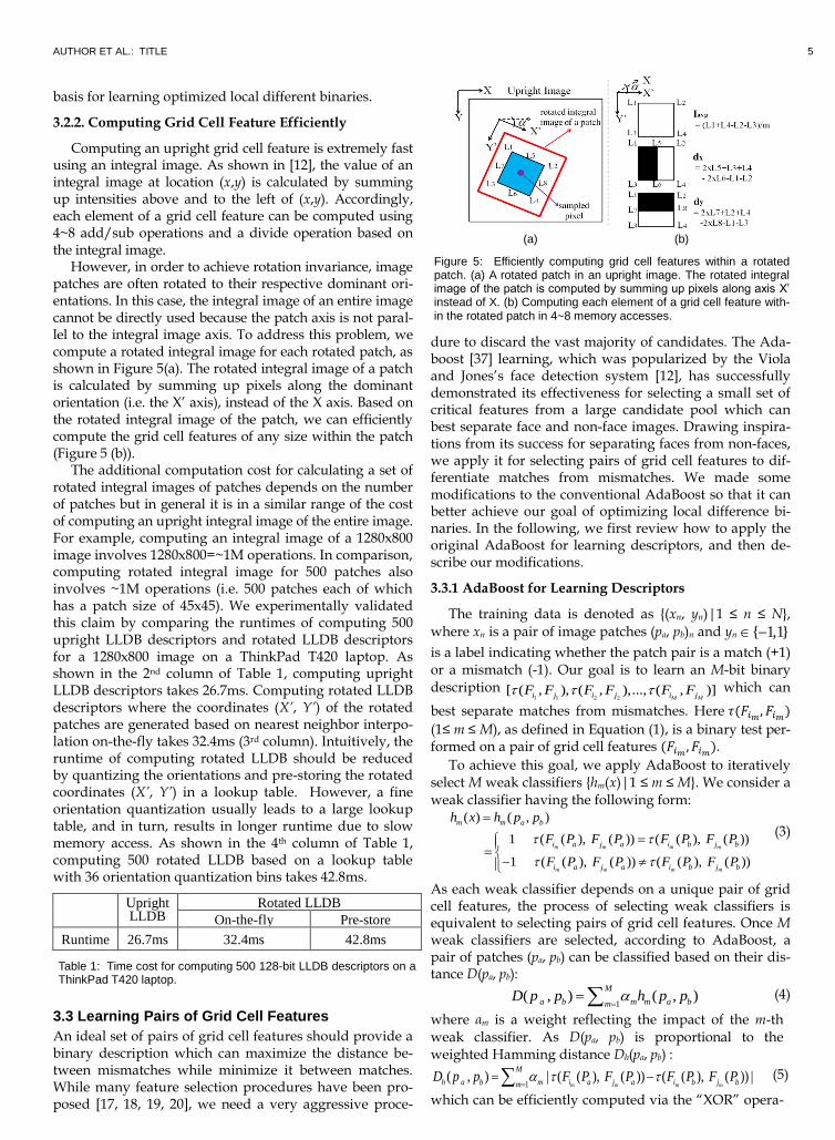
However, in order to achieve rotation invariance, image patches are often rotated to their respective dominant ori-entations. In this case, the integral image of an entire image cannot be directly used because the patch axis is not paral-lel to the integral image axis. To address this problem, we compute a rotated integral image for each rotated patch, as shown in Figure 5(a). The rotated integral image of a patch is calculated by summing up pixels along the dominant orientation (i.e. the X’ axis), instead of the X axis. Based on the rotated integral image of the patch, we can efficiently compute the grid cell features of any size within the patch (Figure 5 (b)).

The additional computation cost for calculating a set of rotated integral images of patches depends on the number of patches but in general it is in a similar range of the cost of computing an upright integral image of the entire image. For example, computing an integral image of a 1280x800 image involves 1280x800=~1M operations. In comparison, computing rotated integral image for 500 patches also involves ~1M operations (i.e. 500 patches each of which has a patch size of 45x45). We experimentally validated this claim by comparing the runtimes of computing 500 upright LLDB descriptors and rotated LLDB descriptors for a 1280x800 image on a ThinkPad T420 laptop. As shown in the 2nd column of Table 1, computing upright LLDB descriptors takes 26.7ms. Computing rotated LLDB descriptors where the coordinates (X’, Y’) of the rotated patches are generated based on nearest neighbor interpo-lation on-the-fly takes 32.4ms (3rd column). Intuitively, the runtime of computing rotated LLDB should be reduced by quantizing the orientations and pre-storing the rotated coordinates (X’, Y’) in a lookup table. However, a fine orientation quantization usually leads to a large lookup table, and in turn, results in longer runtime due to slow memory access. As shown in the 4th column of Table 1, computing 500 rotated LLDB based on a lookup table with 36 orientation quantization bins takes 42.8ms.

3.3 Learning Pairs of Grid Cell Features

An ideal set of pairs of grid cell features should provide a binary description which can maximize the distance be-tween mismatches while minimize it between matches. While many feature selection procedures have been pro-posed [17, 18, 19, 20], we need a very aggressive proce-

dure to discard the vast majority of candidates. The Ada-boost [37] learning, which was popularized by the Viola and Jones’s face detection system [12], has successfully demonstrated its effectiveness for selecting a small set of critical features from a large candidate pool which can best separate face and non-face images. Drawing inspira-tions from its success for separating faces from non-faces, we apply it for selecting pairs of grid cell features to dif-ferentiate matches from mismatches. We made some modifications to the conventional AdaBoost so that it can better achieve our goal of optimizing local difference bi-naries. In the following, we first review how to apply the original AdaBoost for learning descriptors, and then de-scribe our modifications.

3.3.1 AdaBoost for Learning Descriptors

The training data is denoted as {(xn, yn)|1 ≤ n ≤ N},

where xn is a pair of image patches (pa, pb)n and yn { 1,1}

is a label indicating whether the patch pair is a match (+1) or a mismatch (-1). Our goal is to learn an M-bit binary description

1 1 2 2[ ( , ), ( , ),..., ( , )]

M Mi j i j i jF F F F F F which can

best separate matches from mismatches. Here 𝜏(𝐹 , 𝐹 )

(1≤ m ≤ M), as defined in Equation (1), is a binary test per-formed on a pair of grid cell features (𝐹 , 𝐹 ).

To achieve this goal, we apply AdaBoost to iteratively select M weak classifiers {hm(x)|1 ≤ m ≤ M}. We consider a weak classifier having the following form:

( ) ( , )

1 ( ( ), ( )) ( ( ), ( ))

1 ( ( ), ( )) ( ( ), ( ))

m m m m

m m m m

m m a b

i a j a i b j b

i a j a i b j b

h x h p p

F P F P F P F P

F P F P F P F P

(3)

As each weak classifier depends on a unique pair of grid cell features, the process of selecting weak classifiers is equivalent to selecting pairs of grid cell features. Once M weak classifiers are selected, according to AdaBoost, a pair of patches (pa, pb) can be classified based on their dis-tance D(pa, pb):

1( , ) ( , )

M

a b m m a bmD p p h p p

(4)

where αm is a weight reflecting the impact of the m-th weak classifier. As D(pa, pb) is proportional to the weighted Hamming distance Dh(pa, pb) :

1( , ) | ( ( ), ( )) ( ( ), ( )) |

m m m m

M

h a b m i a j a i b j bmD p p F P F P F P F P

(5)

which can be efficiently computed via the “XOR” opera-

(a) (b)

Figure 5: Efficiently computing grid cell features within a rotated patch. (a) A rotated patch in an upright image. The rotated integral image of the patch is computed by summing up pixels along axis X’ instead of X. (b) Computing each element of a grid cell feature with-in the rotated patch in 4~8 memory accesses.

Upright LLDB

Rotated LLDB

On-the-fly Pre-store

Runtime 26.7ms 32.4ms 42.8ms

Table 1: Time cost for computing 500 128-bit LLDB descriptors on a ThinkPad T420 laptop.

6 IEEE TRANSACTIONS ON JOURNAL NAME, MANUSCRIPT ID

tions. In practice, we use Dh(pa, pb) for better efficiency. The key of AdaBoost is the selection of weak classifi-

ers, which is determined in the process of optimizing an objective function. A common objective function used in the conventional AdaBoost procedure is an exponential loss function L over the training data:

1

1( )

2

1

M

n m m nmy h xN

nL e

(6)

To optimize L in Equation (6), in each round of selection AdaBoost selects one pair of grid cell features to form a weak classifier which minimizes the sum of weighted misclassification error εm =∑ 𝑤

( ) 𝐼(ℎ (𝑥 ) ≠ 𝑦 ). Here

𝑤 ( )

is the weight of the n-th training sample in iteration m and is updated iteratively in each round according to Equation (7) to place greater emphasis on those samples incorrectly classified by the previously selected features.

1 1

1( )

( ) ( 1) 2n m m ny h x

m m

n nw w e

(7)

This scheme implicitly reduces correlations among select-ed features as the feature selected in each round tends to classify the training samples in a different way from the ones selected in the previous rounds. A weight αm is cal-culated according to Equation (8) to indicate the impact of the m-th selected feature on the final classification result.

𝛼 = ln(

) (8)

There are three limitations for directly applying the conventional AdaBoost procedure to select local differ-ence binary descriptors:

(1) It’s highly desirable to use Hamming distance as the distance metric so that two local difference binary de-scriptors can be compared with ultra-high efficiency via the XOR and bit count operations. However, the conventional AdaBoost associates a weight αm with each bit of a descriptor, which makes the distance significantly more complex. Directly ignoring the weights (i.e, setting αm = 1 for all m=1,… ,M) is a sim-ple solution. However, this simple solution inevita-bly degrades the matching accuracy. To reduce the performance degradation, it’s desirable to have small differences among the weights so that quantizing all of them to 1 for fast distance estimation between de-scriptors would not degrade the matching accuracy too much. Unfortunately, the conventional AdaBoost automatically generates αm according to the classifica-tion error 𝜀 in each iteration, without providing us a knob to control its value.

(2) To optimize both LDB’s footprint and performance, it’s desirable to have a proper decreasing rate of the objective function for each new iteration. On one hand, a fast decreasing rate can achieve a low classifi-cation error with a smaller number of features, i.e. a small footprint. On the other hand, an excessively fast decreasing rate may lead to a rapid overfit to the training data, adversely limiting the descriptor’s per-formance (i.e. the objective function stops decreasing at a point where the training error is still large). However, the conventional AdaBoost does not offer a

systematical way to control the decreasing rate of the objective function.

(3) The appearance diversity of matching patches is usu-ally larger than that of faces. As a result, the conven-tional AdaBoost would demand much more training data with greater diversity to learn a sufficiently dis-tinctive descriptor. However, this would make the training time impractically long. We observed in our experiment that given 42,588 candidate features and 12,000 training data (~83% being mismatches), a simi-lar amount of candidate features and training data used in Viola and John’s face detection system [12], the conventional AdaBoost can only learn a very short descriptor (around 48bits) and the objective function stops decreasing at that point while the training error is still high. Increasing the training data size to 120,000 increases the training time by 10X, while the training error is only slightly reduced.

To address the above limitations, we made some modifi-cations to the conventional AdaBoost, which are de-scribed in the following subsection.

3.3.2 Modifications

We introduce a variable β and rewrite the objective function as:

1( )

2

1

M

n m m nmy h xN

nL e

(9)

Accordingly, αm and 𝑤 ( )

are computed as:

𝛼 =

ln(

). (10)

1 1 ( )( ) ( 1) 2

n m m ny h xm m

n nw w e

(11)

Details of the derivation of αm and 𝑤 ( )

are given in the Appendix.

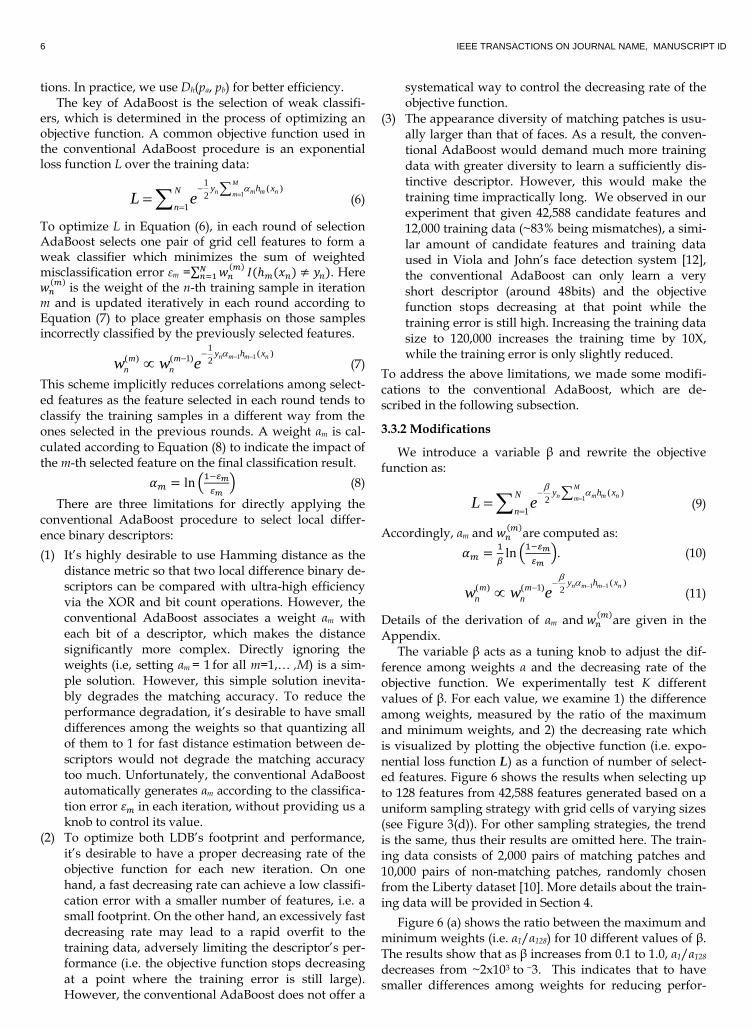
The variable β acts as a tuning knob to adjust the dif-ference among weights α and the decreasing rate of the objective function. We experimentally test K different values of β. For each value, we examine 1) the difference among weights, measured by the ratio of the maximum and minimum weights, and 2) the decreasing rate which is visualized by plotting the objective function (i.e. expo-nential loss function L) as a function of number of select-ed features. Figure 6 shows the results when selecting up to 128 features from 42,588 features generated based on a uniform sampling strategy with grid cells of varying sizes (see Figure 3(d)). For other sampling strategies, the trend is the same, thus their results are omitted here. The train-ing data consists of 2,000 pairs of matching patches and 10,000 pairs of non-matching patches, randomly chosen from the Liberty dataset [10]. More details about the train-ing data will be provided in Section 4.

Figure 6 (a) shows the ratio between the maximum and minimum weights (i.e. α1/α128) for 10 different values of β. The results show that as β increases from 0.1 to 1.0, α1/α128

decreases from ~2x103 to ~3. This indicates that to have smaller differences among weights for reducing perfor-

AUTHOR ET AL.: TITLE 7

mance degradation, a large β is preferred. Figures 6 (b) and (c) show the exponential loss function L for 10 differ-ent values of β. When β is between 0.1 and 0.5 (Figure 6 (b)) a larger β makes the loss function L decrease faster. Therefore, within this range a larger β is preferred since fewer features are needed to achieve the same training error. When β is between 0.5 and 1.0 (Figure 6 (c)), a smaller β makes the loss function saturates later and gives a smaller training error at the saturation point. Therefore, within the range between 0.5 and 1.0, a smaller β is pre-ferred. To summarize the results in Figures 6 (a)-(c), by adjusting the value of β we can limit the differences among weights so that quantizing all of them to 1 for fast distance estimation between descriptors would not de-grade the matching accuracy too much. Furthermore, the value of β can be tuned to explore the tradeoff between the descriptor’s footprint and performance to meet the requirements of various applications.

We also provide a simple solution to maintain a rea-

sonable training complexity and meanwhile learn a suffi-

ciently distinctive descriptor: instead of learning a full

descriptor using a huge amount of training data, we learn

several sub-descriptors using smaller training sets and

concatenate them together to form a distinctive one. More

specifically, we prepare several training sets and based on

each training set we learn a sub-descriptor. The learning process of each sub-descriptor stops once the objective function saturates. This idea is motivated by [12], which leverages a cascade of classifiers and learns classifiers of each stage based on a small amount of training data. In a practical implementation, we utilize the minimum classi-fication error to determine whether the objective function saturates or not. Once the minimum classification error is over 0.5 (i.e. the selected weak classifier is not better than a random guess), the process switches to a new training set.

Pseudo-code 1 details our procedure for selecting pairs of grid cell features.

4 EXPERIMENTS

In this section, we provide experimental details for learn-ing optimized local different binaries. Then we compare

the performance of LLDB with the state-of-the-art binary descriptors for scalable matching and pairwise image matching.

4.1 Learning Local Different Binaries

We first describe the training data, testing data, experi-mental setup and measurement. Then we evaluate the performance of different sampling strategies, grid cell features and pair selection schemes.

4.1.1 Training Data and Testing Data

We use the Liberty data set [10] as a source of training data for the AdaBoost learning. The Liberty dataset con-tains 450,092 patches, sampled densely from multiple images of the 3D scene of Statue of Liberty. The dataset also includes ground truth data indicating the match and mismatch information. The major transformations in the Liberty dataset include scaling, illumination changes and

Pseudo Code 1: AdaBoost-based Feature Selection

Input: training data T = {(xn, yn) | xn = (pa, pb) is a pair of patches, yn = 1 if xn is a match; otherwise is yn = -1, 1≤ n ≤ |T|} Output: M pairs of grid cell features

Step 1. Compute N-bit strings for patches in T. Step 2. For n = 1 to |T|

Assign weight 𝑤 ( )

= 1/|T| to training data Tn. Step 3. For m = 1 to M

a) For feature pair (𝐹 , 𝐹 ), k = 1 to N

- Classify all xn according to Equation (3) - Compute the classification error εb

εb(𝐹 , 𝐹 ) =∑ 𝑤 ( )

𝐼(ℎ (𝑥 ) ≠ 𝑦 )

b) Find a feature pair (𝐹 , 𝐹 ) which gives

minimum classification error ɛm.

(𝐹 , 𝐹 ) = argmin 𝜀 (𝐹 , 𝐹 )

εm= 𝜀 (𝐹 , 𝐹 )

c) If ɛm < 0.5 - For n = 1 to |T|

Update 𝑤 ( ) according to Equation (11)

- Compute αm according to Equation (10) Else

- Discard (𝐹 , 𝐹 ) , switch to a new train

ing set and go back to a)

(a) (b) (c)

Figure 6: (a) Weight ratio α1/α128 (i.e. weight gap) as a function of the tunning knob β. Exponential loss function L as a function of number of selected features (b) when β/2 = 0.1~0.5 and (c) when β/2 = 0.5~1.0. Note that the exponential loss function L is normalized such that the largest entry of L is equal to 1.

8 IEEE TRANSACTIONS ON JOURNAL NAME, MANUSCRIPT ID

viewpoint changes. These transformations commonly exist in MAR applications, thus training descriptors using this dataset can help optimize the performance for practi-cal application scenarios.

We test the performance of our LLDB using 228 pairs of Document-Natural images. Each pair is generated by man-ually capturing two images of an original image from the Document-Natural dataset [36] (Figure 7 - up) with up to ±45o orientation changes and 0.8x~2.0x scaling changes ((Figure 7 - down)).

4.1.2 Experimental Setup and Measurement

In the training phase, we randomly chose 2,000 pairs of matching patches as positive data and 10,000 pairs of non-matching patches as negative data. More negatives are selected since in practice there are significantly more mismatches than matches for most matching tasks. For each sampling strategy (Figure 3), we learn the best M pairs of grid cell features out of 42,588 available pairs. In this experiment, we set M = 32, yielding 32-bit binary de-scriptors. For descriptors of other lengths (64, 128 and 256), we provide detailed evaluation in Sec. 5.2. We set β to 0.5 for all the following experiments as it gives a rela-tively small differences among weights (as shown in Fig-ure 6 (a)) and meanwhile provides a fast decreasing rate of the objective function and a minimum training error (as shown in Figures 6 (b) and (c)).

For each testing image, we detect 1,000 points using an oFAST [4] detector (scales = 4 and scale factor = 1.2). For each point in an image, we perform brute-force matching based on the Hamming distance to find its nearest neigh-bor (NN) on its paired image. Then we verify the match-ing points using RANSAC, and remove the outliers as false matches. Denoting the total number of matching points as N and the number of correct matches as nc, we evaluate the performance of descriptors using the ratio of correct matches nc/N.

4.1.3 Results

Table 2 shows the ratio of correct matches obtained by LLDB for different combinations of sampling strategies and grid cell features. First, we compare the performance of three different location distributions. With keeping all other settings kept the same, the Uniform distribution shows better performance than the Circular (i.e. BRISK Circular) and Retinal distributions for most cases. One possible explanation is that the Circular and Retinal dis-tribution are designed to be more robust with respect to

rotation and viewpoint changes. However, in this exper-iment rotation changes are compensated by aligning patches to dominant orientations and the viewpoint changes are relatively small (In Sec. 4.3 we will show that for images with large viewpoint changes, the Retinal dis-tribution outperforms the Uniform distribution). The Cir-cular and Retinal distributions, which lose more detailed information in the outer region, may lead to less distinc-tive descriptors if details in the outer region are informa-tive and useful.

Second, we examine the use of fixed and varying grid cell size on the descriptor’s performance. In general, us-ing varying sizes can slightly improve the performance of binary descriptors by 0.75% to 6.5%. This makes sense since the outer region is easier to be contaminated by noises, due to translation changes, than the inner region. Using a large smoothing factor can reduce these noises and thus increase the robustness.

Finally, we compare the performance of using only in-tensity summation Iave, with that of using all three grid cell features Iavg, dx and dy. The results in the last two col-umns of Table 2 show that using Iavg +dx + dy can improve the performance by 1.4% to 11.4%. This gain is achieved by the introduction of image gradients.

Table 3 shows the ratio of correct matches for different pair selection schemes: random selection, variance-correlation-based method employed in ORB and FREAK, and our modified AdaBoost method. Table 3 reports the results based on the Uniform distribution, fixed grid cell size and all three grid cell features. For other combina-tions, the trend is consistent. The results show that Ada-Boost learning achieves much better performance than the other two selection schemes. This validates our claim that comparing to existing schemes, the modified Ada-Boost is more capable of choosing a small subset of criti-cal pairs out of a huge number of candidates and facilitat-ing a systematic exploration in a large design space.

4.2 Evaluation of Scalable Matching

In this section we show that LLDB outperforms its com-

Selection Method

Random Variance- Cor-relation [4]

Modified AdaBoost

nc/N 53.7 50.9 67.3

Table 3: The ratio of correct matches for three pair selection schemes. The Uniform distribution, fixed smoothing factor and both types of Harr-like features are used in this test.

Figure 7: Exemplar images from (up) the Document-Natural data-base, (bottom) testing images.

Sampling Strategy Grid Cell Features

Location Distribution

Grid Cell Size Iavg Iavg + dx + dy

Uniform

Circular

Retinal

fixed

fixed

fixed

66.4

62.4

62.5

67.3

66.5

66.6

Uniform Circular Retinal

varying varying varying

66.9 63.2 66.1

70.9 70.4 68.8

Table 2: The ratio of correct matches for different combinations of sampling strategies and grid cell features.

AUTHOR ET AL.: TITLE 9

petitors in Nearest-Neighbor (NN) matching over a large database. The better distinctiveness of LLDB accounts for the superior performance. We start with a brief descrip-tion of Locality Sensitive Hashing (LSH), the indexing structure used for large-scale NN matching.

4.2.1 Locality Sensitive Hashing for LLDB

LSH [25] is a widely used technique for approximate NN search. The key of LSH is a hash function, based on which similar descriptors can be hashed into the same bucket of a hash table while different ones will be stored in different buckets. To find the NN of a query descriptor, we first retrieve its matching bucket and then check all the descriptors within this bucket using a brute-force matching.

For binary features, the hash function is usually a sub-set of bits from the original bit string: buckets of a hash table contain descriptors with a common sub-bit-string. The size of the subset, i.e. hash key size, determines a maximum Hamming distance among descriptors within the same buckets. To improve the chance that a correct NN can be retrieved by LSH, i.e. detection rate of NN, two techniques - multi-table and multi-probe [26] are usually used. Multi-table stores the database descriptors in several hash tables, each of which leverages a different hash function. In the query phase, each query descriptor is hashed into a bucket of every hash table and checks the matches within them. Multi-table improves the detection rate of NN at the cost of linearly increased memory usage and matching time. Multi-probe examines both the bucket in which a query descriptor falls and the neighboring buckets. While multi-probe would result in more matches to check, it actually allows for less hash tables and thus less memory usage. In addition, it enables larger key size and therefore smaller buckets and fewer matches to check per bucket.

4.2.2 Experiment Setup and Measurement

We use the query time per feature and detection rate of true NN to evaluate the matching performance. The evaluation is based on 228 images from Document-Natural images for the database and 228 synthetically generated query imag-es by applying 30 degrees rotation and motion blur (radi-us = 3, sigma = 8 and angle = 4) to the original Document-Natural images, implemented by ImageMagick [27]. To obtain the ground truth of true NN for each keypoint from a query image, we infer its corresponding points on its matched database image using the known homogra-phy between them.

We compare the matching performance of three ver-sions of LLDB with state-of-the-art binary descriptors LDB, ORB, BRISK and FREAK. We use the OpenCV3.2.1 implementations and the default settings for the ORB and FREAK descriptors and the source code from [11] for the BRISK descriptor. For LLDB, we use three types of grid cell features and grid cell of different sizes (i.e. Figure 3 (d), (e) and (f)) for all sampling distributions. For all de-scriptors, we use the same length, i.e. 256 bits.

We tune the LSH parameters: the hash key size and the number of probes, to adjust the detection rate and query

time. A larger hash key size reduces the number of matches to check and hence reduces the runtime per que-ry, but it may also divide true NNs into different buckets, leading to a lower detection rate. Increasing the number of probes improves the detection rate at a cost of longer runtime, which is linearly proportional to the number of probes. In OpenCV 2.3.1 [14], the number of probes is specified through the parameter multi-probe level. Setting level to 0 indicates only the bucket where a query de-scriptor falls is checked, level=1 denotes that the neighbor-ing buckets with 1-bit difference is also examined, and so on and so forth. In the experiment, we used five hash tables and for each table we set the key size as 12, 16, and 18 and the multi-probe level as 0, 1 and 2, yielding 9 sets of LSH parameters in total.

4.2.3 Matching Speed vs. Detection Rate of NN

Figure 8 plotted the results of various methods based on the query time per feature and detection rate of true NN. First, we evaluated the performance of LLDB using three different location distributions: LLDB-U, LLDB-R and LLDB-C. LLDB-U stands for LLDB descriptors using the Uniform distribution. Similarly, LLDB-R and LLDB-C are descriptors using the Retinal and Circular distributions respectively. Given the same LSH parameter setting, LLDB-U achieves a higher detection rate and shorter que-ry time than LLDB-R and LLDB-C. For example, for the setting of the multi-probe level being 2 and the key size

Figure 9: The distributions of the LSH bucket size for the Document-Natural image dataset. LLDB-U give much more uniform buckets than ORB, BRISK, FREAK and LDB, thus improving the query speed.

Figure 8: Runtime vs. detection rate for various methods. Five hash tables are used to store the database with each table containing 456k entries. Therefore, nearest neighbors are searched over 2.3M entries. 9 different sets of LSH parameters are used: the hash key size being 12, 16, and 18 and the multi-probe level being 0, 1, and 2 for each key size.

10 IEEE TRANSACTIONS ON JOURNAL NAME, MANUSCRIPT ID

being 12, LLDB-U retrieves 31% true NNs, while LLDB-R and LLDB-C detect only 26.4% and 24.5% true NNs, re-spectively. With respect to the query time, LLDB-U takes 4.2ms, which is around 22% shorter than LLDB-R (5.4ms) and LLDB-C(5.5 ms). The faster runtime of LLDB-U is most likely due to its better discriminative ability, which reduces the number of descriptors to check in each hash bucket. To further validate this, we plotted the distribu-tions of the bucket sizes in Figure 9. We observed that LLDB-U has more small-sized buckets than LLDB-R and LLDB-C.

Second, we compare the performance of LLDB-U with the other four descriptors. Given the same LSH settings, LLDB-U is much faster for NN search than ORB, BRISK, FREAK and LDB. For example, for the setting of the probe level being 2 and the key size of 12, LLDB-U only takes 4.2ms per query, while FREAK, BRISK, ORB and LDB takes 6.8ms, 8.7ms, 8.8 and 5.6ms, respectively. That is, LLDB-U achieves a 1.3x ~ 2.1x speedup in NN detec-tion its competitors. Regarding the detection rate, LLDB-U also outperforms other descriptors for every LSH set-tings.

4.3 Evaluation for Pairwise Image Matching

In this section, we compare the robustness of LLDB with its competitors to general transformations that commonly exist in practical application scenarios.

4.3.1 Dataset

The evaluation was performed using 6 image sequenc-es [16]. The sequences are divided into 4 categories:

Viewpoint changes: the data sets are Graffiti and Wall;

Image blur: the data set are Trees and Bikes; Compression artifacts: the data set is Jpg; Illumination changes: the data set is Light.

Each sequence contains 6 images. For each sequence, we match the first image to the remaining five, yielding five image pairs per sequence, denoted by pair 1/n (2 ≤ n ≤ 6). The five pairs are sorted in order of ascending diffi-

culty. More specifically, Graffiti and Walls are sorted in order of increasing viewpoint changes to the first image, Trees and Bikes are sorted in increasing image blur, and Light and Jpg are in order of increasing illumination changes and compression artifacts, respectively.

4.3.2 Experiment Setup and Measurement

For each image, we use oFAST detector to detect 1000 keypoints, each of which is then described using a 32-bit binary string. Similar to Sec. 4.1.2, for each keypoint in the first image we find its NNs in the other five images based on brute-force matching. To obtain the ground truth of correct matches, for each keypoint in the first image, we infer its corresponding point in each of the other five im-ages using the known homography between them. The robustness of descriptors is evaluated based on the ratio of correct matches. Here we define a match is correct if the identified NN points are within a predefined distance range (e.g. 10 pixels in this test) to the inferred points.

4.3.3 Results

Figure 10 shows the ratio of correct matches for 6 image sequences. First, we examine the performance for the Graffiti and Wall sequences, which mainly contain view-point changes. Results show that LLDB-R outperforms the other competing descriptors. The results support the following two conclusions: 1) for large viewpoint changes the Retinal distribution offers superior robustness to the other two distributions, 2) LLDB-R has greater robustness comparing to existing binary descriptors. Second, we ex-amine the performance for the remaining image sequenc-es. For these sequences, LLDB-U shows superior perfor-mance to other binary descriptors. The results also show that the Uniform distribution offers better tolerance against image blur, illumination changes and compres-sion artifacts than the other two distributions. Therefore, different distributions may have respective advantages in handling different types of distortions. Our framework can automatically select an optimized set of pairs for all candidate distributions.

Figure 10: The ratio of correct matches obtained by LLDB, REAK, BRISK, ORB, and LDB for the six image sequences. In general, LLDB-R achieves the best performance for Graffiti and Wall sequences which have viewpoint changes (except for Graffiti ½ which has relative small viewpoint changes), and LLDB-U outperforms other descriptors for the Light, Trees, Bikes and JPG sequences.

AUTHOR ET AL.: TITLE 11

5 APPLICATION TO MOBILE AUGMENTED REALITY

We apply LLDB to scalable MAR applications by imple-menting a conventional AR pipeline: we first detect oFAST points and LLDB descriptors for a captured image frame. Then we match it to our database and return the database image with most and sufficient number of matches as a potential recognized result. Finally, we per-form RANSAC [33] to validate the result and have a pose estimate. Once the object is recognized, it is tracked from the next frame by matching features of consecutive frames. The recognizer and tracker of AR are executed complementarily during the entire process: the recognizer is activated whenever the tracker fails or new objects oc-cur and the tracker bridges the recognized results and speeds up the process.

In the following subsections, we evaluate the perfor-mance of scalable object recognition and tracking indi-vidually.

5.1 Object Recognition on Mobile Devices

We first describe the database, the query set, experi-mental setup and measurement metrics used for our evaluation, and then provide results.

5.1.1 Experiment Setup

We evaluate the performance of mobile object recogni-

tion using the 228 Document-Natural images (Figure 12(a))

and 228 testing images (see Figure 12 (b) and (c)). Each

testing image is generated by manually captured a pic-

ture of a database image with 0.8x~2.0x scaling changes

and up to ±45o rotations. In mobile applications, the cap-

tured images are very likely to be blurry due to the

movement of the capturing device. In order to mimic the

motion blur distortions and test the robustness of de-

scriptors to these distortions, we implemented the distor-

tions using ImageMagic [15] with the setting of radius =

3, sigma = 8 and angle = 4, and applied them to each test-

ing image.

We extract 2,000 features on each database image. All

the database features are stored in an LSH indexing struc-

ture, consisting of 5 hash tables with 2.3M entries in total.

For all the hash tables, we set the key size as 18 and the

multi-probe level as 1. We extract 500 features on each

testing image. For each testing feature, we find its NN

using LSH and remove false matches whose Hamming

distance is greater than a threshold. Finally, all remaining

matches are verified by RANSAC. As in previous exper-

iments, LLDB-C achieves the worst performance compar-

ing to LLDB-U and LLDB-R, we remove it from this test.

All experiments were performed on the Motorola Xoom1 tablet, which runs Android 3.0 Honeycomb, fea-tures 1GB RAM and a dual-core ARM Cortex-A9 running at 1GHz clock rate. While there are multi-cores in the pro-cessor, we use only one core in our experiments. Figure 11 displays pictures of our object recognition system run-ning on the Motorola Xoom1 tablet. Figure 12 (b) and (c) show some exemplar recognized query images with scal-ing and rotations, respectively.

5.1.2 Results

Table 4 shows the detection rate when varying the de-

scriptor length from 32bits to 256bits (Note: the precision

of all descriptors are about the same, which is above 90%,

after RANSAC verification). Two observations can be

made from the results. First, for descriptors of short

length, i.e. 32bits and 64bits, LLDB-U has a distinct ad-

vantage over LLDB-R and other competing descriptors. In

particular, the detection rate achieved by LLDB-U of

32bits is 76.2%, which is 26% higher than LLDB-R, and

25.3%, 45.4%, 67.8% and 9.5% higher than FREAK, BRISK,

ORB and LDB, respectively. This demonstrates that

LLDB-U is more suitable than its competitors for applica-

tions which demand small footprint, such as apps run-

ning on mobile devices or using large-scale databases.

Second, for descriptors of longer length, i.e. 128bits and

256bits, LLDB-U still outperforms other descriptors, but

the gap becomes smaller. One explanation for the smaller

gap is that as the number of bits increases, the selection

task for AdaBoost becomes more difficult, yielding an

error rate very close to 0.5. In these cases, the selected

features become trivial, having small contributions for

improving the distinctiveness. How to address this prob-

lem is our future work.

Table 5 shows the query time per image when varying

the descriptor length. The results show that for all de-

Descriptor FREAK BRISK ORB LDB LLDB-U

Time(ms) 61 120 63 70 77

Table 6: Runtime (ms) for computing 256-bit binary descriptors.

Binary Descriptor

32bits 64bits 128bits 256bits

FREAK BRISK ORB LDB

21.1 17.6 7.5

25.1

60.8 52.4 45.4 69.6

85.5 82.5 72.2 90.7

92.5 89.4 86.3 92.7

LLDB-R

LLDB-U

17.6 28.6

56.4 76.2

78.4 89.0

83.7 93.8

Table 4: Detection Rate Comparison: matching 228 manually captured images to the Document-Natural images.

Binary Descriptor

32bits 64bits 128bits 256bits

FREAK BRISK ORB LDB

103 98 75 56

130 196 149 72

332 224 222 100

365 277 231 141

LLDB-R LLDB-U

44 37

52 40

84 53

93 71

Table 5: Query Time (ms) Comparison: matching 228 manually captured images to the Document-Natural images.

12 IEEE TRANSACTIONS ON JOURNAL NAME, MANUSCRIPT ID

scriptors lengths, LLDB-U takes least runtime for recog-

nizing targets from the database. For instance, for 256-bit

descriptors the query time of LLDB-U is only 71ms on the

tablet, which is 5.1X faster than FREAK, 3.9X faster than

BRISK, 3.25X faster than ORB and 2X faster than LDB.

The faster runtime of LLDB-U is due to its better discrim-

inative ability, which helps reduce the number of de-

scriptors to check in each hash bucket.

Table 6 shows the runtime of computing 500 256-bit bi-

nary descriptors. In general, the computational efficiency

of LLDB-U and other descriptors is comparable. FREAK

achieves the fastest runtime (i.e. 61ms). In comparison,

LLDB-U is slightly slower (i.e. 77ms). But FREAK is less

robust and distinctive than LLDB-U, as shown in previ-

ous sections. As a result, it usually incurs longer runtime

for the entire process than LLDB-U. For example, to rec-

ognize 228 objects on the tablet, FREAK costs 426ms for

the entire process, while LLDB-U only takes 148ms.

5.2 Real-Time Patch Tracking on Mobile Devices

Tracking on mobile devices involves matching the live

frames to a previously captured frame. As consecutive

frames usually have large content overlaps, it’s often less

challenging for tracking to achieve satisfactory matching

accuracy than recognition: the photometric changes (e.g.

lighting differences) and geometric changes (e.g. scaling)

are smaller and more predictable. Therefore, in the exper-

iment we extracted fewer oFAST points (200) for tracking

than for recognition (500). Then we compute the LLDB-U

descriptor for each point and search its NN in the previ-

ous frame using a brute-force method for descriptor

matching. The top-ranked putative matches (e.g. 40

matches with the shortest distances in our experiment)

are then validated by homography estimation based on

RANSAC.

Figure 13 shows 40 top-ranked putative matches of

LLDB-U between consecutive frames. The green lines

indicate correct matches that are consistent with homog-

raphy estimation via RANSAC, i.e. inliers, and the red

lines denote the false matches, i.e. outliers. In general,

LLDB-U generates more correct matches on natural imag-

es than on document images. One possible explanation is

that some patches of document images capture the same

character from two different words (e.g. two A’s, one is

from the word “And” and the other one is from “Apple”),

leading to a mismatch. Statistically, LLDB-U generates

68% correct matches out of the top 40 matches. A high

inlier ratio makes the RANSAC algorithm converges

quick, yielding a short verification and estimation

runtime. On a Motorola Xoom tablet, brute-force match-

ing 200 64-bit LLDB-U descriptors of two images takes 13

ms and the subsequent RANSAC estimation for the top40

matches takes 65 ms.

6 CONCLUSIONS

In this paper, we introduce a new binary descriptor,

named LLDB, which achieves higher discriminative abil-

ity, while maintaining similar construction efficiency,

than the state-of-the-art binary descriptors. The superior

performance of LLDB is achieved by three folds: 1) it uti-

lizes both average intensities and gradients, 2) it adopts a

much denser grid cell sampling, and 3) it learns opti-

mized pairs of grid cell features from the labeled exam-

ples using a modified AdaBoost procedure. Various sam-

pling strategies for designing binary descriptors can be

seamlessly plugged into the learning framework and easi-

ly investigated. Comparing to existing approaches, which

only explore in a very limited design space due to signifi-

cant manually efforts and ad hoc schemes, our method

facilitates a systematic exploration in a much larger space,

providing much richer sources for designing robust and

distinctive binary descriptors.

LLDB is demonstrated through a scalable recognition

task and a pariwise image matching task. Due to its better

distinctiveness, LLDB exhibits both faster runtime and

higher accuracy than existing descriptors in recognizing

query images from a database with 2.3M descriptors. For

pairwise image matching, LLDB also outperforms its

competitors.

Though we demonstrated LLDB to MAR applications

using a conventional pipeline, LLDB can be directly in-

corporated into a more advanced flow, e.g. a unified

recognition-and-tracking flow, to further reduce the time

cost for feature detection and description by exploiting

the temporary coherency between consecutive frames.

We will explore this direction in the future.

REFERENCES

[1] Bay, H., Ess, A., Tuytelaars, T. and Gool, L.V., SURF: Speeded-

(a) robust to rotation changes (b) robust to scaling (c) robust to viewpoint changes (d) robust to occlusions

Figure 11: Pictures of our object recognition system based on 64-bit LLDB-U on Motorola Xoom1 tablet at run-time. The green lines demote the matching points between the camera-captured object (left) and the recognized object (right).

AUTHOR ET AL.: TITLE 13

Up Robust Features. In Proc. of ECCV’06.

[2] Lowe, D. G., Distinctive Image Features from Scale-Invariant

Keypoints. In IJCV, vol. 60, no. 2, pp. 91-110, 2004.

[3] Calonder, M., Lepetit, V., Strecha, C., and Fua, P., Brief: Binary

Robust Independent Elementary Features. In Proc. of ECCV’10.

[4] Rublee, E., Rabaud, V., Konolige, K., and Bradski, G., ORB: an

Efficient Alternative to SIFT or SURF. In Proc. of ICCV’11, Barce-

lona, Spain.

[5] Leutenegger, S., Chli, M., Siegwart, R., BRISK: Binary Robust

Invariant Scalable Keypoints. In Proc. of CVPR’11.

[6] Alahi, A., Ortiz, R., and Vandergheynst, P., FREAK: Fast Reti-

nal Keypoint, In Proc. of CVPR’12.

[7] Yang, X. and Cheng, K. T., LDB: An Ultra-Fast Feature for Scal-

able Augmented Reality on Mobile Device. In Proc. of IS-

MAR’12.

[8] Calonder, M., Lepetit, V., Konolige K., Bowman, J., Mihelich, P.,

and Fua, P., Compact Signatures for High-Speed Interest Point

Description and Matching, In Proc. of ICCV’09.

[9] Winder, S., and Brown, M., Learning Local Image Descriptors,

In Proc. of CVPR’07. [10] Winder, S., Hua, G., and Brown, M., Picking the Best DAISY, In

Proc. of CVPR’09.

[11] Babenko, B., Dollar, P., and Belongie, S., Task Specific Local

Image Matching. In Proc. of ICCV’07.

[12] Viola, P., and Jones, M., Robust Real-time Object Detection, In

IJCV, vol. 57, no. 2, pp. 137-154, May 2004.

[13] Mikolajczyk, K., and Schmid, C., A Performance Evaluation of

Local Descriptors, In TPAMI, vol. 27, no. 27, Oct. 2005.

[14] OpenCV2.3.1,http://sourceforge.net/projects/opencvlibrary.

[15] ImageMagic, http://www.imagemagick.org/script/index.php

[16] ImageSequences, http://www.robots.ox.ac.uk/~vgg/research

[17] Brown, M., Hua, G. and Winder, S, Discriminative Learning of Local

Image Descriptors, In Trans. of PAMI, 2011.

[18] Ke, Y., and Sukthankar, R., PCA-SIFT: A More Distinctive Represen-

tation for Local Image Descriptors. In Proc. of CVPR’04.

[19] Jia, Y., Huang, C. and Darrell, T., Beyond Spatial Pyramids: Recep-

tive Field Learning for Pooled Image Features, In Proc. of CVPR’12.

[20] Simonyan, K., Vedali, A. and Zisserman, A., Descriptor Learning

Using Convex Optimisation, In Proc. of ECCV’12.

[21] Wagner, D., Reitmayr, G., Mulloni, A., Drummond, T. and

Schmalstieg, D., Pose tracking from natural features on mobile

phones. In Proc. of ISMAR’08.

[22] Wagner, D., Schmalstieg, D., and Bischof, H., Multiple Target Detec-

tion and Tracking with Guaranteed Framerates on Mobile Phones. In

Proc. of ISMAR’09.

[23] Wagner, D., Mulloni, A., Langlotz, T., and Schmalstieg, D., Real-time

Panoramic Mapping and tracking on Mobile Phones. In Proc of IEEE

VR’10.

[24] Klein, G., and Murray, D., Parallel tracking and mapping on a camera

phone. In Proc. of ISMAR’09, Orlando, October.

[25] Ta, D.N., Chen, W.C., Gelfand, N., and Pulli, K., SURFTrac: Effi-

cient Tracking and Continuous Object Recognition using Local Fea-

ture Descriptors. In Proc. of CVPR’09.

[26] Takacs, G., Chandrasekhar, V., and Tsai, S., Unified Real-Time

Tracking and Recognition with Rotation-Invariant Fast Features. In

Proc. of CVPR’10.

[27] Torralba, A., Fergus, R., Weiss, Y., Small Codes and Large Databases

for Recognition. In Proc. of CVPR’08.

[28] Taylor, S., Rosten, E., Drummond, T., Robust feature matching in

2.3us. In Proc. of CVPR’09.

[29] Lepetit, V., Lagger, P., and Fua, P., Randomized Trees for Real-time

Keypoint Recognition. In Proc. of CVPR’05, pp. 775-781.

[30] Pilet, J., and Saito, H., Virtually Augmenting Hundreds of Real Pic-

tures: An Approach based on Learning, Retrieval, and Tracking. In

Proc. of VR’10.

[31] Rosten, E., Porter, R., and Drummond, T., Faster and Better: A ma-

chine learning approach to corner detection. IEEE Trans. PAMI,

32:105–119, 2010.

[32] Chum, O., and Matas, J., Matching with PROSAC – progressive

sample consensus. In Proc. of CVPR’05, volume 1, pages 220–226.

[33] Fischler, M. A. and Bolles, R. C., Random Sample Consensus: A

Paradigm for Model Fitting with Applications to Image Analysis and

Automated Cartography. Comm. of the ACM 24 (6), pp. 381–395,

June, 1981.

[34] Gionis, A., Indyk, P., and Motwani, R., Similarity search in high

dimensions via hashing. In Proc. of VLDB’99.

[35] Lv, Q., Josephson, W., Wang, Z., Charikar, M., and Li, K., Multi-

probe LSH: efficient indexing for high-dimensional similarity search.

In Proc. of VLDB’07.

Figure 12: (a) Exemplar images from the Document-Natural database, (b) and (c) recognized query images with scaling and rotations, re-spectively. We use 64-bit LLDB-U in this experiment. The green rectangles illustrate the pose between the camera and the recognized object, and red dots denote the matched points.

14 IEEE TRANSACTIONS ON JOURNAL NAME, MANUSCRIPT ID

[36] Yang, X., Liu, Q., Liao, C. Y. and Cheng, K. T., Large-Scale EMM

Identification Based on Geometry-Constrained Visual Word Corre-

spondence Voting, In Proc. of ICMR’11, Trento, Italy.

[37] Freund, Y. and Schapire, E. R., A Decision-Theoretic Generalization

of On-Line Learning and an Application to Boosting. In Journal of

Computer and System Sciences, 55: 119-139, 1997.

[38] Shakhnarovich, G., Learning Task-Specific Similarity, PhD Thesis,

MIT, 2005.

[39] Trzcinski, T., Christoudias, M., Lepetit, V., and Fua, P., Learning

Image Descriptors with the Boosting-Trick, In Proc. of NIPS’12.

[40] Ali, K., Fleuret, F., Hasler, D. and Fua, P., A Real-Time Deformable

Detector. In Trans. of PAMI, 34(2): 225-239, 2012.

APPENDIX

We use the following modified objective function L:

1( )

2

1

M

n m m nmy h xN

nL e

(12)

When selecting the weak classifier hm at step m, the object function can be re-written as the following which sepa-rates out the contribution of classifier hm:

1

1( ) ( )

2 2

1=

m

n j j n n m m njy h x y h xN

nL e e

(13)

Since the m-1 weak classifiers already selected previously won’t change in the future iterations, we can replace the first m-1 terms with a constant:

1

1( )

( ) 2

m

n j j njy h x

m

nw e

(14)

Accordingly, Equation (13) can be expressed as:

( )

( ) 2

1=

n m m ny h xN m

nnL w e

(15)

We can split Equation (15) into two terms: one for data correctly classified by hm and the other for those misclassi-fied:

( ) ( )2 2

: ( ) : ( )=

m m

m n n m n n

m m

n nn h x y n h x yL w e w e

(16)

Rearranging these terms, we have

( )2 2

1

( )2

1

( ) ( ( ) )

m m

m

N m

n m n nn

N m

nn

L e e w I h x y

e w

(17)

Optimizing for L in Equation (17) with respect to hm is

equivalent to minimizing∑ 𝑤 ( )𝐼(ℎ (𝑥 ) ≠ 𝑦 ) , which

is the weighted misclassification error. The optimal val-ue for αm can be derived by solving dL/dαm = 0. That is,

( )2 2

( )2

( ) ( ( ) )2

02

m m

m

mmn m n nn

m

mmnn

dLe e w I h x y

d

e w

(18)

After dividing both sides by ( )/ 2 m

m nnw and denoting

εm as the normalized weighted misclassification error, ( )

( )

( ( ) )m

n m n nnm m

nn

w I h x y

w

(19)

we can finally arrive at:

2 2 2 0m m m

m me e e

(20)

11ln m

m

m

(21)

Xin Yang received her PhD degree in University of California, Santa Barbara in 2013. Currently she is working as a Post-doc in Learning-based Multimedia Lab at UCSB. Her research interests include mobile computer vision and its applica-tion to mobile augmented reality, large-scale content-based image retrieval. She is a student member of IEEE and a member of ACM. Kwang-Ting (Tim) Cheng worked at Bell La-boratories in Murray Hill, N J, from 1988 to 1993 and joined the faculty at UC Santa Barbara in 1993 where he is currently Acting Associate Vice Chancellor for Research and Professor of Elec-trical and Computer Engineering. He was the Founding Director (1999-2002) of UCSB's Com-puter Engineering program and former Chair (2005-2008) of the ECE Department. He also

served as Visiting Professor at Univ. of Tokyo Japan, Beijing Univer-sity China, National TsingHua University, Taiwan, and Hong Kong University of Science and Technology. He has published over 350 technical papers, co-authored five books and holds 12 U.S. Patents. Cheng, a fellow of IEEE, served as Editor-in-Chief for IEEE Design and Test of Computers and currently serves on the editorial boards of several IEEE and ACM journals.

Figure 13: 40 top-ranked putative matches of LLDB-U descriptors between two consecutive frames. The green lines indicate correct matches, i.e. inliers, and the red lines denote false matches, i.e. outliers. More correct matches are detected on natural images than on document imag-es by LLDB-U.