Learning Long-Term Dependencies with GradientDescent is Di�cultYoshua Bengioy, Patrice Simardy, and Paolo FrasconizyAT&T Bell LaboratorieszDip. di Sistemi e Informatica, Universit�a di FirenzeAbstractRecurrent neural networks can be used to map input sequences to output se-quences, such as for recognition, production or prediction problems. However, prac-tical di�culties have been reported in training recurrent neural networks to performtasks in which the temporal contingencies present in the input/output sequences spanlong intervals. We show why gradient based learning algorithms face an increasinglydi�cult problem as the duration of the dependencies to be captured increases. Theseresults expose a trade-o� between e�cient learning by gradient descent and latch-ing on information for long periods. Based on an understanding of this problem,alternatives to standard gradient descent are considered.Paper to appear in the special issue on Recurrent Networks of the IEEE Transactions onNeural Networks1

1 IntroductionWe are interested in training recurrent neural networks to map input sequences to outputsequences, for applications in sequence recognition, production or time-series prediction.All of the above applications require a system that will store and update context infor-mation, i.e., information computed from the past inputs and useful to produce desiredoutputs. Recurrent neural networks are well suited for those tasks because they have aninternal state that can represent context information. The cycles in the graph of a recur-rent network allow it to keep information about past inputs for an amount of time that isnot �xed a-priori, but rather depends on its weights and on the input data. In contrast,static networks (i.e., with no recurrent connection), even if they include delays (such asTime Delay Neural Networks [15]), have a �nite impulse response and can't store a bit ofinformation for an inde�nite time. A recurrent network whose inputs are not �xed butrather constitute an input sequence can be used to transform an input sequence into anoutput sequence while taking into account contextual information in a exible way. Werestrict here our attention to discrete-time systems.Learning algorithms used for recurrent networks are usually based on computing the gra-dient of a cost function with respect to the weights of the network [22, 21]. For example,the back-propagation through time algorithm [22] is a generalization of back-propagationfor static networks in which one stores the activations of the units while going forward intime. The backward phase is also backward in time and recursively uses these activations tocompute the required gradients. Other algorithms, such as the forward propagation algo-rithms [14, 23], are much more computationally expensive (for a fully connected recurrentnetwork) but are local in time, i.e., they can be applied in an on-line fashion, produc-ing a partial gradient after each time step. Another algorithm was proposed [10, 18] for2

training constrained recurrent networks in which dynamic neurons { with a single feedbackto themselves { have only incoming connections from the input layer. It is local in timelike the forward propagation algorithms and it requires computation only proportional tothe number of weights, like the back-propagation through time algorithm. Unfortunately,the networks it can deal with have limited storage capabilities for dealing with generalsequences [7], thus limiting their representational power.A task displays long-term dependencies if computation of the desired output at time tdepends on input presented at an earlier time � � t. Although recurrent networks can inmany instances outperform static networks [4], they appear more di�cult to train optimally.Earlier experiments indicated that their parameters settle in sub-optimal solutions whichtake into account short-term dependencies but not long-term dependencies [5]. Similarresults were obtained by Mozer [19]. It was found that back-propagation was not su�cientlypowerful to discover contingencies spanning long temporal intervals. In this paper, wepresent experimental and theoretical results in order to further the understanding of thisproblem.For comparison and evaluation purposes, we now list three basic requirements for a para-metric dynamical system that can learn to store relevant state information. We requirethat1. the system be able to store information for an arbitrary duration,2. the system be resistant to noise (i.e., uctuations of the inputs that are random orirrelevant to predicting a correct output).3. the system parameters be trainable (in reasonable time).Throughout the paper, the long-term storage of de�nite bits of information into the state3

variables of the dynamic system is referred to as information latching. A formalization ofthis concept, based on hyperbolic attractors, is given in section 4.1.The paper is divided in �ve sections. In Section 2 we present a minimal task that can besolved only if the system satis�es the above conditions. We then present a recurrent networkcandidate solution and negative experimental results indicating that gradient descent isnot appropriate even for such a simple problem. The theoretical results of Section 4 showthat either such a system is stable and resistant to noise or, alternatively, it is e�cientlytrainable by gradient descent, but not both. The analysis shows that when trying to satisfyconditions (1) and (2) above, the magnitude of the derivative of the state of a dynamicalsystem at time t with respect to the state at time 0 decreases exponentially as t increases.We show how this makes the back-propagation algorithm (and gradient descent in general)ine�cient for learning of long term dependencies in the input/output sequence, hence failingcondition (3) for su�ciently long sequences. Finally, in Section 5, based on the analysisof the previous sections, new algorithms and approaches are proposed and compared tovariants of back-propagation and simulated annealing. These algorithms are evaluated onsimple tasks on which the span of the input/output dependencies can be controlled.2 Minimal Task Illustrating the ProblemThe following minimal task is designed as a test that must necessarily be passed in or-der to satisfy the three conditions enumerated above. A parametric system is trained toclassify two di�erent sets of sequences of length T . For each sequence u1; : : : ; uT the classC(u1; : : : ; uT ) 2 f0; 1g depends only on the �rst L values of the external input:C(u1; : : : ; uT ) = C(u1; : : : ; uL):4

We suppose L �xed and allow sequences of arbitrary length T � L. The system shouldprovide an answer at the end of each sequence. Thus, the problem can be solved onlyif the dynamic system is able to store information about the initial input values for anarbitrary duration. This is the simplest form of long-term computation that one may aska recurrent network to carry out. The values uL+1; : : : ; uT are irrelevant for determiningthe class of the sequences. However, they may a�ect the evolution of the dynamic systemand eventually erase the internally stored information about the initial values of the input.Thus the system must latch information robustly, i.e., in such a way that it cannot beeasily deleted by events which are unrelated with the classi�cation criterion. We assumehere that for each sequence, ut is zero-mean Gaussian noise for t > L.The third required condition is learnability. There are two di�erent computational aspectsinvolved in this task. First, it is necessary to process u1; � � � ; uL in order to extract someinformation about the class, i.e., perform classi�cation. Second, it is necessary to store suchinformation into a subset of the state variables (let us call them latching state variables) ofthe dynamic system, for an arbitrary duration. For this task, the computation of the classdoes not require accessing latching state variables. Hence the latching state variables donot need to a�ect the evolution of the other state variables. Therefore, a simple solutionto this task may use a latching subsystem, fed by a subsystem that computes informationabout the class.We are interested in assessing learning capabilities on this latching problem independentlyon a particular set of training sequences, i.e. in a way that is independent on the speci�cproblem of classifying u1; : : : ; uL. Therefore we will focus here only on the latching subsys-tem. In order to train any module feeding the latching subsystem, the learning algorithmshould be able to transmit error information (such as gradient) to such a module. An im-portant question is thus whether the learning algorithm can propagate error information5

to a module that feeds the latching subsystem and detects the events leading to latching.Hence, instead of feeding a recurrent network with the input sequences de�ned as abovewe use only the latching subsystem as a test system and we reformulate our minimal taskas follows. The test system has one input ht and one output xt (at each discrete time stept). The initial inputs ht, for t � L, are values which can be tuned by the learning algorithm(e.g., gradient descent) whereas ht is Gaussian noise for L < t � T . The connection weightsof the test system are also trainable parameters. Optimization is based on the cost functionC = 12Xp (xpT � dp)2where p is an index over the training sequences and dp is a target of +0:8 for sequence ofclass 1 and �0:8 for sequences of class 0.In this formulation, ht (t = 1; : : : ; L) represent the result of the computation that extractsthe class information. Learning ht directly is an easier task than computing it as a paramet-ric function ht(ut; �) of the original input sequence and learning the parameters �. In fact,the error derivatives @C@ht (as used by backpropagation through time) are the same as if htwere obtained as a parametric function of ut. Thus, if ht cannot be directly trained as pa-rameters in the test system (because of vanishing gradient), they clearly cannot be trainedas a parametric function of the input sequence in a system that uses a trainable moduleto feed a latching subsystem. The ability of learning the free input values h1; : : : ; hL is ameasure of the e�ectiveness of the gradient of error information which would be propagatedfurther back if the test system were connected to the output of another module.6

3 Simple Recurrent Network Candidate SolutionWe performed experiments on this minimal task with a single recurrent neuron, as shownin Fig. 1a. Two types of trajectories are considered for this test system, for the two classes(k = 0; k = 1): xkt = f(akt ) = tanh(akt )akt = w f(akt�1) + hkt t = 1 : : : Ta00 = a10 = 0 (1)If w > 1=f 0(0) = 1, then the autonomous dynamic of this neuron has two attractorsx > 0 and �x that depend on the value of the weight w [7, 8] (they can be easily obtainedas non zero intersections of the curve x = tanh(a) with the line x = a=w). Assuming thatthe initial state at t = 0 is x0 = �x, it can be shown [8] that there exists a value h� > 0of the input such that, (1) xt maintains its sign if jhtj < h� 8t , and, (2) there exists a�nite number of steps L1 such that xL1 > x if ht > h� 8t � L1. A symmetric case occursfor x0 = �x. h� increases with w. For �xed w, the transient length L1 decreases with jhtj.Thus the recurrent neuron of Fig. 1a. can robustly latch one bit of information, representedby the sign of its activation. Storing is accomplished by keeping a large input (i.e., largerthan h� in absolute value) for a long enough time. Small noisy inputs (i.e., smaller than h�in absolute value) cannot change the sign of the activation of the neuron, even if appliedfor arbitrary long time. This robustness essentially depends on the nonlinearity.The recurrent weight w is also trainable. The solution for T � L requires w > 1 toproduce two stable attractors x and �x. Larger w correspond to larger critical value h�and, consequently, more robustness against noise. The trainable input values must bringthe state of the neuron towards x or �x in order to robustly latch a bit of informationagainst the input noise. For example this can be accomplished by adapting, for t = 1; : : : ; L,7

h1t � H and h0t � �H, where H > h� controls the transient duration towards one of thetwo attractors.In Fig. 1b we show two sample sequences that feed the recurrent neuron. As stated insection 2, hkt are trainable for t � L and samples from a Gaussian distribution with mean0 and variance s for t > L. The values of ht for t � L were initialized to small uniformrandom values before starting training. A set of simulations were carried out to evaluate thee�ectiveness of back-propagation (through time) on this simple task. In a �rst experimentwe investigated the e�ect of the noise variance s and of di�erent initial values w0 for theself loop weight (see also [3].) A density plot of convergence is shown in Fig. 2a, averagedover 18 runs for each of the selected pairs (w0; s). It can be seen that convergence becomesvery unlikely for large noise variance or small initial values of w. L = 3 and T = 20 werechosen in these experiments.In Fig. 2b, we show instead the e�ect of varying T , keeping �xed s = 0:2 and w0 = 1:25.In this case the task consists in learning only the input parameters ut. As explained insection 2, If the learning algorithm is unable to properly tune the inputs ut, then it will notbe able to learn what should trigger latching in a more complicated situation. Solving thistask is a minimum requirement for being able to transmit error information backwards,towards modules feeding the latch unit.When T becomes large it is extremely di�cult to attain convergence. These experimentalresults show that even in the very simple situation where we want to robustly latch on 1bit of information about the input, gradient descent on the output error fails for long-terminput/output dependencies, for most initial parameter values.8

4 Learning to Latch with Dynamical SystemsIn this section, we attempt to understand better why learning even simple long-term de-pendencies with gradient descent appears to be so di�cult. We discuss the general caseof a real-time recognizer based on a parametric dynamical system. We �nd that the con-ditions under which a recurrent network can robustly store information (in a way de�nedbelow, i.e. with hyperbolic attractors) yield a problem of vanishing gradients that canmake learning very di�cult.We consider a non-autonomous discrete-time system with additive inputs:at =M(at�1) + ut (2)and the corresponding autonomous dynamicsat =M(at�1) (3)where M is a nonlinear map, and at and ut are n-vectors representing respectively thesystem state and the external input at time t.To simplify the analysis presented in this section, we consider only a system with additiveinputs. However, a dynamic system with non-additive inputs, e.g., at = N(at�1; ut�1), canbe transformed into one with additive inputs by introducing additional state variables andcorresponding inputs. Suppose at 2 Rn and ut 2 Rm. The new system is de�ned by theadditive inputs dynamics a0t = N 0(a0t�1) + u0t where a0t = (at; yt) is a n+m-vector state, andthe �rst n elements of u0t = (0; ut) 2 Rn+m are 0. The new map N 0 can be de�ned interms of the old map N as follows: N 0(a0t�1) = (N(at�1; yt�1); 0), with m zeroes for thelast elements of N 0(). Hence we have yt = ut. Note that a system with additive inputswith a map of the form of N 0() can be transformed back into an equivalent system withnon-additive inputs. Hence without loss of generality we can use the model in eq. 2.9

In the next subsection, we show that only two conditions can arise when using hyperbolicattractors to latch bits of information. Either the system is very sensitive to noise, orthe derivatives of the cost at time t with respect to the system activations a0 convergeexponentially to 0 as t increases.This situation is the essential reason for the di�culty in using gradient descent to train adynamical system to capture long-term dependencies in the input/output sequences.4.1 AnalysisIn order to latch a bit of state information one wants to restrict the values of the systemactivity at to a subset S of its domain. In this way, it will be possible to later interpret at inat least two ways: inside S and outside S. To make sure that at remains in such a region,the system dynamics can be chosen such that this region is the basin of attraction of anattractor (or of an attractor in a sub-manifold or subspace of at's domain). To \erase"that bit of information, the inputs may push the system activity at out of this basin ofattraction and possibly into another one. In this section, we show that if the attractoris hyperbolic (or can be transformed into one, e.g. a stable periodic attractor), then thederivatives @at@a0 quickly vanish as t increases. Unfortunately, when these gradients vanish,training becomes very di�cult because the in uence of short-term dependencies dominatesin the weights gradient.De�nition 1 A set of points E is said to be invariant under a map M if E =M(E).De�nition 2 A hyperbolic attractor is a set of points X invariant under the di�erentiablemap M , such that 8a 2 X, all eigenvalues of M 0(a) are less than 1 in absolute value.10

An attractor X may contain a single point (�xed point attractor), a �nite number of points(periodic attractor), or an in�nite number of points (chaotic attractor). Note that a stableand attracting �xed point is hyperbolic for the map M , whereas a stable and attractingperiodic attractor of period l for the mapM is hyperbolic for the mapM l. For a recurrentnet, the kind of attractor depends on the weight matrix. In particular, for a network de�nedby at =W tanh(at�1) + ut , ifW is symmetric and its minimum eigenvalue is greater than-1, then the attractors are all �xed points [17]. On the other hand, if jW j < 1 or if thesystem is linear and stable, the system has a single �xed point attractor at the origin.De�nition 3 The basin of attraction of an attractor X is the set �(X) of points a con-verging to X under the map M , i.e., �(X) = fa : 8�;9l;9x 2 X s:t: kM l(a)� xk < �g.De�nition 4 We call �(X), the reduced attracting set of a hyperbolic attractor X, the setof points y in the basin of attraction of X, such that 8l � 1, all the eigenvalues of (M l)0(y)are less than 1.Note that by de�nition, for a hyperbolic attractor X, X � �(X) � �(X).De�nition 5 A system is robustly latched at time t0 to X, one of several hyperbolic at-tractors, if at0 is in the reduced attracting set of X under a map M de�ning the autonomoussystem dynamics.For the case of non-autonomous dynamics, it remains robustly latched to X as long as theinputs ut are such that at 2 �(X) for t > t0. Let us now see why it is more robust to storea bit of information by keeping at in �(X), the reduced attracting set of X.Theorem 1 Assume x is a point of Rn such that there exist an open sphere U(x) centeredon x for which jM 0(z)j > 1 for all z 2 U(x). Then there exist y 2 U(x) such thatkM(x)�M(y)k > kx� yk. 11

Proof: see the Appendix.This theorem implies that for a hyperbolic attractor X, if a0 is in �(X) but not in �(X),then the size of a ball of uncertainty around a0 will grow exponentially as t increases,as illustrated in �gure 3(a). Therefore, small perturbations in the input could push thetrajectory towards another (possibly wrong) basin of attraction. This means that thesystem will not be resistant to input noise. What we call input noise here may be simplycomponents of the inputs that are not relevant to predict the correct future outputs. Incontrast, the following results show that if a0 is in �(X), at is guaranteed to remain withina certain distance of X when the input noise is bounded.De�nition 6 A map M is contracting on a set D if 9� 2 [0; 1) such thatkM(x)�M(y)k � �kx� yk 8x; y 2 D.Theorem 2 LetM be a di�erentiable mapping on a convex set D. If 8x 2 D; jM 0(x)j < 1,then M is contracting on D.Proof: See [20].A crucial element in this analysis, is to identify the conditions in which one can robustlylatch information with an attractor:Theorem 3 Suppose the system is robustly latched to X, starting in state a0, and theinputs ut are such that for all t > 0, kutk < bt, where bt = (1 � �t)d. Let ~at be theautonomous trajectory obtained by starting at a0 and no input u. Also suppose 8y 2Dt; jM 0(y)j < �t < 1, where Dt is a ball of radius d around at. Then at remains inside aball of radius d around ~at, and this ball intersects X when t!1.Proof: see the Appendix. 12

The above results justi�es the term \robust" in our de�nition of robustly latched system:as long as at remains in the reduced attracting set �(X) of a hyperbolic attractor X, abound on the inputs can be found that guarantees at to remain within a certain distance ofsome point in X, as illustrated in �gure 3(b). The smaller is jM 0(y)j in the region aroundat, the looser is the bound bt on the inputs, meaning that the system is more robust toinput noise. On the other hand, outside �(X) but in �(X), M is not contracting, it isexpanding, i.e., the size of a ball of uncertainty grows exponentially with time.We now show the consequences of robust latching, i.e., vanishing gradient:Theorem 4 If the input ut is such that a system remains robustly latched on attractor Xafter time 0, then @at@a0 ! 0 as t!1.Proof: see the Appendix.The results in this section thus show that when storing one or more bit of information ina way that is resistant to noise, the gradient with respect to past events rapidly becomesvery small in comparison to the gradient with respect to recent events. In the next sectionwe discuss how that makes gradient descent on parameter space (e.g., the weights of anetwork) ine�cient.4.2 E�ect on the Weight GradientLet us consider the e�ect of vanishing gradients on the derivatives of a cost Ct at time twith respect to parameters of a dynamical system, say a recurrent neural network withweights W : @Ct@W =X��t @Ct@a� @a�@W =X��t @Ct@at @at@a� @a�@W (4)Suppose we are in the condition in which the network has robustly latched. Hence for a13

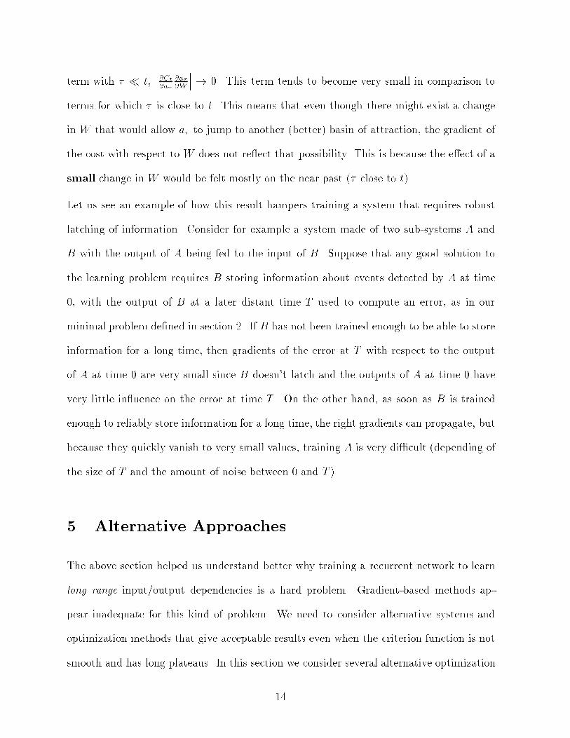
term with � � t, ���@Ct@a� @a�@W ��� ! 0. This term tends to become very small in comparison toterms for which � is close to t. This means that even though there might exist a changein W that would allow a� to jump to another (better) basin of attraction, the gradient ofthe cost with respect to W does not re ect that possibility. This is because the e�ect of asmall change in W would be felt mostly on the near past (� close to t).Let us see an example of how this result hampers training a system that requires robustlatching of information. Consider for example a system made of two sub-systems A andB with the output of A being fed to the input of B. Suppose that any good solution tothe learning problem requires B storing information about events detected by A at time0, with the output of B at a later distant time T used to compute an error, as in ourminimal problem de�ned in section 2. If B has not been trained enough to be able to storeinformation for a long time, then gradients of the error at T with respect to the outputof A at time 0 are very small since B doesn't latch and the outputs of A at time 0 havevery little in uence on the error at time T . On the other hand, as soon as B is trainedenough to reliably store information for a long time, the right gradients can propagate, butbecause they quickly vanish to very small values, training A is very di�cult (depending ofthe size of T and the amount of noise between 0 and T ).5 Alternative ApproachesThe above section helped us understand better why training a recurrent network to learnlong range input/output dependencies is a hard problem. Gradient-based methods ap-pear inadequate for this kind of problem. We need to consider alternative systems andoptimization methods that give acceptable results even when the criterion function is notsmooth and has long plateaus. In this section we consider several alternative optimization14

algorithms for this purpose, and compare them to two variants of back-propagation.One way to help in the training of recurrent networks is to set their connectivity and initialweights (and even constraints on the weights) using prior knowledge. For example, thisis accomplished in [8] and [11] using prior rules and sequentiality constraints. In fact, theresults in this paper strongly suggest that when such prior knowledge is given, it shouldbe used, since the learning problem itself is so di�cult. However, there are many instanceswhere many long-term input/output dependencies are unknown and have to be learnedfrom examples.5.1 Simulated AnnealingGlobal search methods such as simulated annealing can be applied to such problems, butthey are generally very slow. We implemented the simulated annealing algorithm presentedin [6] for optimizing functions of continuous variables. This is a \batch learning" algorithm(updating parameters after all examples of the training set have been seen). It performsa cycle of random moves, each along one coordinate (parameter) direction. Each point isaccepted or rejected according to the Metropolis criterion [13]. New points are selectedaccording to a uniform distribution inside a hyperrectangle around the last point. Thedimensions of the hyperrectangle are updated in order to maintain the average percentageof accepted moves at about one-half of the total number of moves. After a certain numberof cycles, the temperature is reduced by a constant multiplicative factor (0.85 in the exper-iments). Training stops when some acceptable value of the cost function is attained, whenlearning gets \stuck" 1, or if a maximum number of function evaluations is performed. A1when the cost value on the last N� points does not change by more than � (a small constant) andthese values are all within � of the current optimal cost value found by the algorithm. In the experiments,� = 0:001 and N� = 4. 15

`function evaluation' corresponds to performing a single pass through the network, for oneinput sequence.5.2 Multi-Grid Random SearchThis simple algorithm is similar to the simulated annealing algorithm. Like simulatedannealing, it tries random points. However, if the main problem with the learning taskswas plateaus (rather than local minima), an algorithm that accepts only points that reducethe error could be more e�cient. This algorithm has this property. It performs a (uniform)random search in a hyperrectangle around the current (best) point. When a better pointis found, it reduces the size of the hyperrectangle (by a factor of 0.9 in the experiments)and re-centers it around the new point. The stopping criterion is the same as for simulatedannealing.5.3 Time-Weighted Pseudo-Newton OptimizationThe pseudo-Newton algorithm [2] for neural networks has the advantage of re-scaling thelearning rate of each weight dynamically to match the curvature of the energy functionwith respect to that weight. This is of interest because adjusting the learning rate couldpotentially circumvent the problem of vanishing gradient. The pseudo-Newton algorithmcomputes a diagonal approximation to the Hessian matrix (second derivatives of the costwith respect to the parameters) and updates parameters according to the following on-linerule: �wi(p) = � �@2C(p)j@w2i j + � � @C(p)@wi (5)where �wi(p) is the update for weight wi after pattern p has been presented, C(p) is the16

cost for pattern p, and � and � are small positive constants. This amounts to computinga local learning rate for each parameter by using the inverse of the second derivative withrespect to each parameter as a normalizing factor. When @2C(p)j@w2i j is small, the curvature issmall (around the current value of w) in the direction corresponding to the wi axis. Hencea larger step can be taken in that direction. This algorithm was tested in the experimentsdescribed in section 5.5. It consistently performs better than standard back-propagationbut still fails more and more as we increase the span of input/output dependencies.This algorithm and our theoretical results of section 4 inspired the following time-weightedpseudo-Newton algorithm. The basic idea is to consider the unfolding of the recurrentnetwork in time, and each instantiation of a weight (at di�erent times) as a separatevariable, albeit with the constraint that these now separate variables should be equal. Tosimplify the problem, we consider here a cost C(p) which depends on the output of thenetwork at the �nal time step of sequence p. Hence the weight update for wi can becomputed as follows: �wi(p) = �Xt �@2C(p)j@w2itj + � � @C(p)@wit (6)where wit is the instantiation for time t of parameter wi. In this way, each (temporal)contribution to �wi(p) is weighted by the inverse curvature with respect to wit, the in-stantiation of parameter wi at time t 2. The reader may compare the above equation withequation 4, where all the temporal contributions are uniformly summed. Consequently,updating w according to equation 6 does not actually follow the gradient (but neitherwould following equation 5). Instead, several gradient contributions are weighted usingsecond derivatives, in order to make faster moves in the atter directions. Like for thepseudo-Newton algorithm of [2], we prefer using a diagonal approximation of the Hessian2The idea of using second derivatives in this way was inspired from discussions with L. Bottou.17

which is cheap to compute and guaranteed to be positive. � is a global learning rate (0.01in our experiments). The constant � is introduced to prevent �w from becoming verylarge (when @2C(p)j@w2itj is very small). However, we found that much better performance canbe attained with the recurrent networks when � is adapted on-line. This prevents themaximum �w from being greater than a certain upper bound (0.3 in the experiments) orsmaller than a certain lower bound (0.001 in the experiments). The constant � is updatedwith a \momentum" term (0.8 in the experiments), in order to prevent it from decreasingtoo rapidly when the �rst and second derivatives vary widely from sequence to sequenceand have very small magnitude (for example when the norm of the weight matrix jW j isless than 1).5.4 Discrete Error PropagationThe analysis of section 4 could suggest that the root of the problem lies in the essentiallydiscrete nature of the process of storing information for an inde�nite amount of time.Indeed, the gradient backpropagated through time vanishes when the system stays in thesame stable state for several time steps. Intuitively, we would like to recover some errorinformation at the time when the input made the system reach that stable state. Insteadof propagating a gradient through di�erentiable units, the algorithm presented here wasexplicitly designed to propagate discrete error information through units that compute anon-di�erentiable function, such as a hard threshold. In this way we hope to �nd algorithmthat directly address the problem of propagating error backwards in time, even though theprocess of robustly storing information appears to have a discrete nature.Other methods have been explored in order to train layered networks of hard thresholdunits. For example, in [1] it is shown how to train two layered networks using a probabilistic18

approach. In [9] a method is proposed that iterates two training steps: adjusting thenetwork internal representation (units activations) and training the parameters to producesuch representation. This algorithm can be applied to recurrent networks as well. Bothmethods take advantage of probabilities in order to make di�erentiable the error function,thus permitting the use of gradient descent. Another approach, proposed in [12], applies totwo layer networks. The space of activities of hidden units is searched in a greedy way inorder reduce output error. An earlier algorithm also related to the one presented here, butbased on the propagation of targets was proposed in [16]. The algorithm introduced here,instead, relies on propagating discrete error information, obtained with a �nite di�erenceapproach.A neural network can be represented as a series of local elements with each a forwardpropagation function and an error propagation function. We will derive these functions fora discrete element and show how they can be used together with standard di�erentiableelements to minimize a cost function. Our building block for discrete elements is thenon-linear threshold function. The forward propagation is given byyi(x) = sign(xi) (7)where yi 2 f�1; 1g is the output of unit i and xi 2 R its input. We are now interested in�nding the discrete counterpart of gradient propagation for this unit. To backpropagatean error signal, we should �rst establish the relation between variations of the output �yiand variations of the input �xi. This can be done in a systematic way. The variation�yi(�xi) can be easily computed from equation 7 by considering under which conditions19

the output y of a discrete threshold unit will change by 2, -2 or 0:�yi = ������������� 2 if xi < 0 and xi +�xi � 0�2 if xi � 0 and xi +�xi < 00 otherwise (8)and from this equation we can compute the desired variation �xi(�yi) of xi when thedesired variation of yi is �yi:�xi = ������������� �� xi if �yi = 2��� xi if �yi = �20 otherwise (9)where � is a positive constant. We now denote by �yi and �xi the desired changes inyi and xi respectively. Let C be a cost function on our system when a certain pattern(sequence) is presented. A \pseudo-gradient" �C�xi should re ect the in uence of a changeof xi on the cost C. In our experiment we set �C�xi to 1�xi(�yi) if �yi 6= 0 and 0 otherwise.To use the \pseudo gradient" we must insure that �yi is in f2;�2; 0g since �xi(�yi) isnot de�ned for other values. This is achieved using a stochastic process. Let's assumethat there exist two constants MIN and MAX such that the error signal �C�yi = gi to bebackpropagated is a real number satisfying MIN � gi �MAX. We de�ne the stochasticfunction �yi = S(gi) which maps gi to f�2; 2g as follows:8>><>>: P (S(gi) = 2) = gi�MINMAX�MINP (S(gi) = �2) = MAX�giMAX�MIN (10)Provided that �2 < MIN and MAX < 2, it is easy to show that the expectation ofS(gi) is exactly gi, even though S(gi)can only take two values (if jgij > 2 the resultingexpected value will be -2 or +2). Furthermore the sum of this \pseudo gradient" overseveral patterns quickly converges to the sum of the continuous valued gi's.20

The non-linear threshold unit can be used in combination with any other di�erentiableelements which backpropagate the gradient in the usual fashion. The important pointis that when a non-linear threshold unit is connected to itself in a loop with a positivegain, two stable �xed points are induced. The \pseudo gradient" along this loop doesn'tvanish with time which is the essential reason for using discrete units. This pseudo-gradientdoesn't vanish along the loop, as can be observed by repetitively applying equations 9 and8 and noting that if the pseudo-gradient is large enough in magnitude then it is alwayspropagated.This approach is in no way optimal and many other discrete error propagation algorithmsare possible. Another very promising approach for instance is the trainable discrete ip- op unit [3] which also preserves error information in time. Our only claim here is thatdiscrete propagation of error o�ers interesting solutions to the vanishing gradient problemin recurrent network. Our preliminary results on toy problems (see next subsection and[3]) con�rm this hypothesis.5.5 Experimental ResultsExperiments were performed to evaluate various alternative optimization approaches onproblems on which one can increase the temporal span of input/output dependencies. Ofcourse, when it is possible, �rst training on shorter sequences helps a lot, but in manyproblems no such \short-term" version of the problem is available. Hence a goal of theseexperiments was to measure how these algorithms can perform when it is not possibleto train using sequences with equivalent short-term dependencies. Experiments were per-formed with and without input noise (uniformly distributed in [-0.2,0.2]) and varying thelength of the input/output sequences. The criteria by which the performance of these al-21

gorithms were measured are (1) the average classi�cation error at the end of training, i.e.,after the stopping criterion has been met (when either some allowed number of functionevaluations has been performed or the task has been learned), (2) the average number offunction evaluations needed to reach the stopping criterion.Experiments were performed on three problems: the Latch problem, the 2-Sequence prob-lem, and the Parity problem. For each of these problems, a suitable architecture was chosenand all algorithms were used to search in the resulting parameter space (except that thediscrete error propagation algorithm used hard threshold neurons instead of symmetricsigmoids). Initial parameters of the networks were randomly generated for each trial (uni-formly between -0.5 and 0.5). The choice of inputs and the noise for each training sequencewas also randomly generated for each trial. The same initial conditions and training setwere used with each of the algorithms (at a given trial). For each trial, a training set wasgenerated with sequences whose length is uniformly distributed between T=2 and T . Thenumber T (maximum sequence length) is displayed in Figure 4. The tasks all involved asingle input and a single output at each time step.Latch Problem The Latch problem is the same as described above in Section 3.Here we considered only three adaptive parameters: the self-loop weight w, the initial inputvalue u1 for \positive" sequences (with positive �nal target), and the initial input value u0for \negative" sequences (with negative �nal target). The network thus had only one unit.2-Sequence Problem The 2-Sequence problem is the following: classify an inputsequence as one of two sequences when given the �rst N elements of this sequence. N variesfrom pattern to pattern and noise may be added to the input. Hence the network can'trely on the last particular values it saw. Instead, early on, it must recognize subsequencesbelonging to one of the two classes and store that information (or update it if con icting22

information arrives) until its output is read out (which may be at any time but is doneonly once per sequence). These initial key subsequences were randomly generated froma uniform distribution in [-1,1]. In all experiments we used a fully connected recurrentnetwork with 5 units and no bias (one of the units received external additive input, i.e.,the network has 25 free parameters).Parity Problem The Parity problem consists in producing the parity of an inputsequence of 1's and -1's (i.e., a 1 should be produced in output if and only if the numberof 1's in the input is odd). The target is only given at the end of the sequence. The lengthof the sequence may vary and the input may be noisy. It is a di�cult problem that haslocal minima (like the XOR problem), and that appears more and more di�cult for longersequences. Most local optimization algorithms tend to get stuck in a local minimum formany initial values of the parameters. The minimal size network that we implementedhas 7 free parameters and 2 units (2 inputs connected to 1 hidden and 1 output units).Although it requires less parameters than the 2-Sequence problem, it is a more di�cultlearning problem.The results displayed in Figure 4 can be summarized as follows:� Although simulated annealing performed well on all problems, it requires an order ofmagnitude more training time than all the other algorithms. This is not surprisingsince it is global search algorithm. The multi-grid algorithm is faster but fails onthe Parity problem, probably because of local minima. It is also interesting to notethat on the Latch problem with simulated annealing, training time increases withsequence length. Although the best solution is the same for all sequence lengths, theerror surface for longer sequences could be more di�cult to search, even for simulatedannealing. 23

� The discrete error propagation algorithm performed reasonably well on all the prob-lems and sequence lengths, and was the only one with simulated annealing that couldsolve the Parity problem. Because it performs an on-line local search it is howevermuch faster than simulated annealing. It seems to be more robust to local minimathan the multi-grid random search.� The pseudo-Newton back-propagation algorithm consistently performs better thanthe standard back-propagation. However, both see their performance worsen whenthe temporal span of input/output dependencies increasing.� The time-weighted pseudo-Newton algorithm appears to perform better than theother two variants of back-propagation but its performance also appears to worsenwith increasing sequence length.6 ConclusionRecurrent networks are very powerful in their ability to represent context, often outperform-ing static networks [4]. However, we have presented theoretical and experimental evidenceshowing that gradient descent of an error criterion may be inadequate to train them fortasks involving long-term dependencies. Assuming hyperbolic attractors are used to storestate information, we found that either the system would not be robust to input noise orwould not be e�ciently trainable by gradient descent when long term context is required.Note that the theoretical results presented in this paper hold for any error criterion andnot only for the mean square error criterion. Two simple generalizations are obtained asfollows. As mentioned in the analysis section, a periodic attractor can be transformed intoa �xed point by subsampling time with the period of the attractor. Hence if corresponding24

�xed point is stable, it is also hyperbolic and our results hold in that case as well. Anotherinteresting case is the situation in which the system doesn't remain long near an attractor,but rather, jumps rapidly from one stable (hyperbolic) attractor to another. This wouldarise for example if the continuous dynamics can be made to correspond to the discretedynamics of a deterministic �nite-state automaton. In that case, our results hold as wellsince the norm of Jacobian of the map derivatives near each of the attractor is less thanone ( @at@at�1 = M 0(at�1)). What remains to be shown is that similar problems occur withchaotic attractors, i.e., that either the gradients vanish or the system is not robust to inputnoise. It is interesting to note that related problems of vanishing gradient may occur indeep feedforward networks (since a recurrent network unfolded in time is just a very deepfeedforward network with shared weights).The result presented here does not mean that it is impossible to train a recurrent networkon a particular task. It says that gradient descent becomes increasingly ine�cient when thetemporal span of the dependencies increases. Furthermore, for a given problem, there aresometimes ways to help the training by setting the network connectivity and initial weights(and even constraints on the weights) using prior knowledge (e.g., [8], [11]). For sometasks, it is also possible to present a variety of examples of the input/output dependencies,including short-term dependencies which are su�cient to infer similar but longer termdependencies. For example, in the Latch problem or the Parity problem, if we start bytraining with short sequences, the system rapidly settles in the correct region of parameterspace.A better understanding of this problem has driven us to design alternative algorithms,such as the time-weighted pseudo-Newton and the discrete error propagation algorithms.In the �rst case, we consider the instantiation of the weights at di�erent times as dif-ferent variables and consider the curvature of the cost function for these variables. This25

information is used to weight the gradient contributions for the di�erent times in such away as to make larger steps in directions where the cost function is atter. The discreteerror propagation algorithm propagates error information through a mixture of discreteand continuous elements. The gradient is locally quantized with a stochastic decision rulethat appears to help the algorithm in locally searching for solutions and getting out of localminima. We have compared these algorithms with standard optimization algorithms on toytasks on which the temporal span of the input/output dependencies could be controlled.The very preliminary results we obtained are encouraging and suggest that there may beways to reconcile learning with storing. Good solutions to the challenge presented here tolearning long-term dependencies with dynamical systems such as recurrent networks mayhave implications for many types of applications for learning systems, e.g., in languagerelated problems, for which long-term dependencies are essential in order to make correctdecisions.AppendixProof of Theorem 1:By hypothesis and de�nition of norm, 9 u s.t. kuk = 1 and kM 0(x)uk > 1. The Taylorexpansion of M at x for small value of � is:M(x+ �u) =M(x) +M 0(x)�u+O(k�uk2) (11)Since U(x) is an open set, 9 � s.t. kO(k�uk2)k < �(kM 0(x)uk�1) and x+�u 2 U(x). Let-ting y = x+�u we can write kM(y)�M(x)�M 0(x)�uk = kO(k�uk2)k < �kM 0(x)uk��or �kM(y)�M(x)�M 0(x)�uk+kM 0(x)�uk > �. This implies using the triangle inequal-ity kM(y)�M(x)k > � = kx� yk.2 26

Proof of Theorem 3:Let us denote by �t the radius of the \uncertainty" ball �t = fa : k ~at � ak < �tg in which weare sure to �nd at, where ~at gives the trajectory of the autonomous system. Let us supposethat at time t, �t < d (this is certainly true at time 0, when ~a0 = a0). By Lagrange's meanvalue theorem and convexity of Dt, 9z 2 Dt s.t.kM(x)�M(y)k � jM 0(z)jkx� yk, but jM 0(z)j < �t by hypothesis. Then by the con-traction theorem [20] we have �t+1 � �td+ bt. Now by hypothesis we have bt = (1 � �t)d,so �t+1 < d. The conclusion of the theorem is then obtained since ~at 2 Dt by our construc-tion above and ~at converges to X for t!1. 2Proof of Theorem 4:By hypothesis and de�nitions 4 and 2, ��� @a�@a��1 ��� = jM 0(a��1)j < 1 for � > 0, hence @at@a0 ! 0as t!1 2.One could however ask what happens when at remains near the boundary between twobasins:Lemma 1 Suppose that for t > 0, a0 and ut are such that at remains on the boundarybetween two basins of attraction for attractors X1 and X2, and there exists an in�nites-imal change in a0 yielding the state into either X1 or X2 and remaining there. Thenlimt!1 ��� @at@a0 ��� =1.It appears that the hypotheses of this lemma will rarely be satis�ed, for two reasons.Firstly, the system evolves in discrete time, making it improbable to obtain at preciselyon the boundary surface. Second, in order to stay on that surface, say S(at) = 0, ut mustsatisfy the equation S(M(at�1) + ut) = 0. Hence the submanifold of values of ut in Rmwhich satisfy this equation has dimension m� 1, thus having null measure.27

Generalization to a Projection of the StateThe results obtained so far can be generalized to the case when a projection Pat of the stateat converges to an attractor under a map M . This would be the case for example when asubset of the hidden units in a recurrent network participate directly in the dynamics of astable attractor. Let P and R be orthogonal projection matrices such thatat = P+zt + R+ytzt = Pat; yt = RatPR+ = 0; RP+ = 0 (12)where A+ denotes the right pseudo-inverse of A, i.e. AA+ = I. Suppose M is such that Pcan be chosen so that zt converges to an attractor Z with the dynamics zt = MP (zt�1) =PtM(P+zt+R+yt) for any yt. Then we can specialize all the previous de�nitions, lemmasand theorems to the subspace zt. When we conclude with these results that @zt@z0 ! 0 , wecan infer that @at@a0 ! R+ @yt@y0R , i.e., that the derivatives of at with respect to a0 depend onlyon the projection of a on the subspace Ra. Hence the in uence of changes in the projectionof a on the subspace Pa is ignored in the computation of the gradient with respect to W ,even though non-in�nitesimal changes in Pa could yield very di�erent results (i.e., jumpinginto a di�erent basin of attraction). Although training can now proceed in some directions,the e�ect of parameters that in uence detecting and storing events for the long-term orswitching between stable states is still not taken very much into account.References[1] P.L. Bartlett, and T. Downs, \Using Random Weights to train Multilayer Networksof Hard-Limiting Units," IEEE Transactions on Neural Networks, vol. 3, no. 2, 1992,pp. 202{210. 28

[2] S. Becker and Y. Le Cun, \Improving the convergence of back-propagation learningwith second order methods", Proceedings of the 1988 Connectionist Models SummerSchool, (eds. Touretzky, Hinton and Sejnowski), Morgan Kaufmann, pp. 29{37.[3] Y. Bengio, P. Frasconi, P. Simard, \The problem of learning long-term dependenciesin recurrent networks", invited paper at the IEEE International Conference on NeuralNetworks 1993, San Francisco, IEEE Press.[4] Y. Bengio, \Arti�cial Neural Networks and their Application to Sequence Recogni-tion," Ph.D. Thesis, McGill University, (Computer Science), 1991, Montreal, Qc.,Canada.[5] Y. Bengio, R. De Mori, G. Flammia, and R. Kompe, \Global Optimization of a NeuralNetwork - Hidden Markov Model Hybrid," IEEE Transactions on Neural Networks,vol. 3, no. 2, 1992, pp. 252{259.[6] A. Corana, M. Marchesi, C. Martini, and S. Ridella, \Minimizing Multimodal Func-tions of Continuous Variables with the Simulated Annealing Algorithm", ACM Trans-actions on Mathematical Software, vol. 13, no. 13, Sept. 1987, pp. 262{280.[7] P. Frasconi, M. Gori, and G. Soda, \Local Feedback Multilayered Networks", NeuralComputation 3, 1992, pp. 120{130.[8] P. Frasconi, M. Gori, M. Maggini, and G. Soda, \Uni�ed Integration of Explicit Rulesand Learning by Example in Recurrent Networks," IEEE Trans. on Knowledge andData Engineering, in press.[9] R.J. Gaynier, and T. Downs, \A Method of Training Multi-layer Networks with Heav-iside Characteristics Using Internal Representations," IEEE International Conferenceon Neural Networks 1993, San Francisco, pp. 1812{1817.29

[10] M. Gori, Y. Bengio and R. De Mori, \BPS: a learning algorithm for capturing thedynamic nature of speech," Proc. IEEE Int. Joint Conf. on Neural Networks, Wash-ington DC, 1989, pp. II.417-II.424.[11] C.L. Giles and C.W. Omlin, \Inserting Rules into Recurrent Neural Networks", NeuralNetworks for Signal Processing II, Proceedings of the 1992 IEEE workshop, (eds. Kung,Fallside, Sorenson and Kamm), IEEE Press, pp. 13-22.[12] T. Grossman, R. Meir and E. Domany, \Learning by choice of internal representation",Neural Information Processing Systems 1, (ed. D.S. Touretzky), pp. 73{80.[13] S. Kirkpatrick, C.D. Gelatt, M.P. Vecchi, \Optimization by simulated annealing",Science 220, 4598 (May 1983), pp.671{680.[14] Kuhn G., \A �rst look at phonetic discrimination using connectionist models withrecurrent links." CCRP { IDA SCIMP working paper No.4/87, Institute for DefenseAnalysis, Princeton, NJ, 1987.[15] K.J. Lang and G.E. Hinton, \The development of the Time-Delay Neural Networkarchitecture for speech recognition", Technical Report CMU-CS-88-152, Carnegie-Mellon University, 1988.[16] Y. Le Cun, \Learning Processes in an Asymmetric Threshold Network", in Disorderedsystems and biological organization, (eds. Bienenstock, E. and Fogelman-Souli�e, F. andWeisbuch, G.), Springer-Verlag, Les Houches, France, 1986, pp. 233-240.[17] C.M. Marcus, F.R. Waugh, and R.M. Westervelt, \Nonlinear Dynamics and Stabilityof Analog Neural Networks", Physica D 51 (special issue), 1991, pp. 234-247.30

[18] Mozer M.C. \A focused back-propagation algorithm for temporal pattern recognition",Complex Systems, 3, 1989, pp. 349-391.[19] Mozer M.C., \Induction of multiscale temporal structure", Advances in Neural Infor-mation Processing Systems 4, (eds. Moody, Hanson, Lippman), Morgan Kaufmann,1992, pp. 275-282.[20] Ortega J.M. and Rheinboldt W.C. Iterative Solution of Non-linear Equations in Sev-eral Variables and Systems of Equations, Academic Press, New York, 1960.[21] Rohwer R. \The `Moving Targets' Training Algorithm", Advances in Neural Informa-tion Processing Systems 2, (ed. Touretzky), Morgan Kaufmann, 1990, pp. 558-565.[22] D.E. Rumelhart, G.E. Hinton and R.J. Williams, \Learning internal representationby error propagation," Parallel Distributed Processing volume 1. Rumelhart D.E. andMcClelland J.L. (eds.), Bradford Books, MIT Press, 1986, pp. 318{362.[23] Williams R.J. and Zipser D. \A learning algorithm for continuously running fullyrecurrent neural networks", Neural Computation, 1, 1989, pp. 270-280.31

xt = f(at) = tanh(at)at = wxt�1 + hth

t1

ht0

ht

w (a)

L T t

tL T

(b)

Figure 1: a) Latching recurrent neuron. b) Sample input to the recurrent neuron. The trainablevalues h1; : : : ; hL (marked in bold) have been tuned by one of the successfully learning simulations.32

0.5 1 1.5 2 2.5

Wo

0

0.2

0.4

0.6

0.8

1

S

(a)

5

10

15

20

25

30

35

40

45

50

55

60 T

(b)

0.2

0.4

0.6

0.8

1

Freq.

Figure 2: Experimental results for the minimal problem. a) Density of training convergence withrespect to the initial weight w0 and the noise variance s (white ) high density), with L = 3 andT = 20. b) Frequency of training convergence with respect to the sequence length T , (with noisevariance s = 0:2, and initial weight w0 = 1:25).33

X

β

Γ

Domain of a t

(a)

X

β

Domain of at

Γ

(b)

|M’|>1

|M’|<1

|M’|<1

|M’|>1

Figure 3: Basin of attraction (�), reduced attracting set (�) of an attractor X. Ball ofuncertainty grows exponentially (a) outside �, but is bounded (b) inside �.34

0 10 20 30 40 50 60 70 80 90 1000.025

0.05

0.1

0.2

0.4

0.8

0 10 20 30 40 50 60 70 80 90 100

0 10 20 30 40 50 60 70 80 90 100 0 10 20 30 40 50 60 70 80 90 100

0 10 20 30 40 50 60 70 80 90 100 0 10 20 30 40 50 60 70 80 90 100

Final Classification Error, Latch Problem # Sequence Presentations, Latch Problem

100

200

400

800

1600

3200

6400

12800

25600

51200

Final Classification Error, 2−Sequence Problem

0.025

0.05

0.1

0.2

0.4

0.8

# Sequence Presentations, 2−Sequence Problem

100

200

400

800

1600

3200

6400

12800

25600

51200

Final Classification Error, Parity Problem

0.025

0.05

0.1

0.2

0.4

0.8

# Sequence Presentations, Parity Problem

100

400

1600

6400

25600

102400

409600

T T

T T

T TFigure 4: Comparative simulation results for: 2 standard back-propagation, 5 pseudo-Newton,4 time-weighted pseudo-Newton, discrete error propagation, � multi-grid random search,jjjjjjjjjjjjjjjj simulated annealing. The horizontal axis (T ) represents maximum sequence length. On theleft, the vertical axis represents classi�cation error after training; on the right, the number ofsequence presentations to reach a stopping criterion.35