Learning Large-Alphabet and Analog Circuits with

Value Injection Queries

Dana Angluin1 James Aspnes1,∗ Jiang Chen2,†

Lev Reyzin1,‡,§

1 Computer Science Department, Yale University{angluin,aspnes}@cs.yale.edu, lev.reyzin@yale.edu

2 Center for Computational Learning Systems, Columbia Universitycriver@cs.columbia.edu

Abstract

We consider the problem of learning an acyclic discrete circuit withn wires, fan-in bounded by k and alphabet size s using value injec-tion queries. For the class of transitively reduced circuits, we developthe Distinguishing Paths Algorithm, that learns such a circuit using(ns)O(k) value injection queries and time polynomial in the number ofqueries. We describe a generalization of the algorithm to the class ofcircuits with shortcut width bounded by b that uses (ns)O(k+b) valueinjection queries. Both algorithms use value injection queries that fixonly O(kd) wires, where d is the depth of the target circuit. We give areduction showing that without such restrictions on the topology of thecircuit, the learning problem may be computationally intractable whens = nΘ(1), even for circuits of depth O(log n). We then apply our large-alphabet learning algorithms to the problem of approximate learningof analog circuits whose gate functions satisfy a Lipschitz condition.Finally, we consider models in which behavioral equivalence queries arealso available, and extend and improve the learning algorithms of [7]to handle general classes of gate functions that are polynomial timelearnable from counterexamples.

∗Supported in part by NSF grant CNS-0435201.†Supported in part by a research contract from Consolidated Edison.‡Supported in part by a Yahoo! Research Kern family Scholarship.§This material is based upon work supported under a National Science Foundation

Graduate Research Fellowship.

1

1 Introduction

We consider learning large-alphabet and analog acyclic circuits in the valueinjection model introduced in [7]. In this model, we may inject values ofour choice on any subset of wires, but we can only observe the one outputof the circuit. However, the value injection query algorithms in that paperfor boolean and constant alphabet networks do not lift to the case when thesize of the alphabet is polynomial in the size of the circuit.

One motivation for studying the boolean network model includes generegulatory networks. In a boolean model, each node in a gene regulatorynetwork can represent a gene whose state is either active or inactive. How-ever, genes may have a large number of states of activity. Constant-alphabetnetwork models may not adequately capture the information present in thesenetworks, which motivates our interest in larger alphabets.

Akutsu et al. [2] and Ideker, Thorsson, and Karp [11] consider the dis-covery problem that models the experimental capability of gene disruptionand overexpression. In such experiments, it is desirable to manipulate asfew genes as possible. In the particular models considered in these papers,node states are fully observable – the gene expression data gives the stateof every node in the network at every time step. Their results show that inthis model, for bounded fan-in or sufficiently restricted gene functions, theproblem of learning the structure of a network is tractable.

In contrast, there is ample evidence that learning boolean circuits solelyfrom input-output behaviors may be computationally intractable. Kearnsand Valiant [15] show that specific cryptographic assumptions imply thatNC1 circuits and TC0 circuits are not PAC learnable in polynomial time.These negative results have been strengthened to the setting of PAC learn-ing with membership queries [8], even with respect to the uniform distri-bution [16]. Furthermore, positive learnability results exist only for fairlylimited classes, including propositional Horn formulas [4], general read onceBoolean formulas [5], and decision trees [9], and those for specific distribu-tions, including AC0 circuits [17], DNF formulas [12], and AC0 circuitswith a limited number of majority gates [13].1

Thus, Angluin et al. [7] look at the relative contributions of full obser-vation and full control of learning boolean networks. Their model of valueinjection allows full control and restricted observation, and it is the modelwe study in this paper. Interestingly, their results show that this model

1Algorithms in both [17] and [13] for learning AC0 circuits and their variants run inquasi-polynomial time.

2

gives the learner considerably more power than with only input-output be-haviors but less than the power with full observation. In particular, theyshow that with value injection queries, NC1 circuits and AC0 circuits areexactly learnable in polynomial time, but their negative results show thatdepth limitations are necessary.

A second motivation behind our work is to study the relative importanceof the parameters of the models for learnability results. The impact ofalphabet size on learnability becomes a natural point of inquiry, and ideasfrom fixed parameter tractability are very relevant [10, 20].

In this paper we show positive learnability results for bounded fan-in,large alphabet, arbitrary depth circuits given some restrictions on the topol-ogy of the target circuit. Specifically, we show that transitively reduced cir-cuits and circuits with bounded shortcut width (as defined in section 2) areexactly learnable in polynomial time, and we present evidence that shortcutwidth is the correct parameter to look at for large alphabet circuits. We alsoshow that analog circuits of bounded fan-in, logarithmic depth, and smallshortcut width that satisfy a Lipschitz condition are approximately learnablein polynomial time. Finally, we extend the results of [7] when behavioralequivalence queries are also available, for both binary and large-alphabetcircuits.

2 Preliminaries

2.1 Circuits

We give a general definition of acyclic circuits whose wires carry valuesfrom a set Σ. For each nonnegative integer k, a gate function of arityk is a function from Σk to Σ. A circuit C consists of a finite set of wiresw1, . . . , wn, and for each wire wi, a gate function gi of arity ki and an orderedki-tuple wσ(i,1), . . . , wσ(i,ki) of wires, the inputs of wi. We define wn to bethe output wire of the circuit. We may think of wires as outputs of gatesin C.

The unpruned graph of a circuit C is the directed graph whose verticesare the wires and whose edges are pairs (wi, wj) such that wi is an inputof wj in C. A wire wi is output-connected if there is a directed path inthe unpruned graph from that wire to the output wire. Wires that are notoutput-connected cannot affect the output value of a circuit. The graph ofa circuit C is the subgraph of its unpruned graph induced by the output-connected wires.

A circuit is acyclic if its graph is acyclic. In this paper we consider

3

only acyclic circuits. If u and v are vertices such that u 6= v and there isa directed path from u to v, then we say that u is an ancestor of v andthat v is a descendant of u. The depth of an output-connected wire wi isthe length of a longest path from wi to the output wire wn. The depth of acircuit is the maximum depth of any output-connected wire in the circuit.A wire with no inputs is an input wire; its default value is given by itsgate function, which has arity 0 and is constant.

We consider the property of being transitively reduced [1] and a gen-eralization of it: bounded shortcut width. Let G be an acyclic directedgraph. An edge (u, v) of G is a shortcut edge if there exists a directedpath in G of length at least two from u to v. G is transitively reduced ifit contains no shortcut edges. A circuit is transitively reduced if its graph istransitively reduced. Note that in a transitively reduced circuit, for everyoutput-connected wire wi, no ancestor of wi is an input of any descendantof wi, otherwise there would be a shortcut edge in the graph of the circuit.

The shortcut width of a wire wi is the number of wires wj such thatwj is both an ancestor of wi and an input of a descendant of wi. (Note thatwe are counting wires, or vertices, not edges.) The shortcut width of acircuit C is the maximum shortcut width of any output-connected wire inC. A circuit is transitively reduced if and only if it has shortcut width 0. Acircuit’s shortcut width turns out to be a key parameter in its learnabilityby value injection queries.

2.2 Experiments on circuits

Let C be a circuit. An experiment e is a function mapping each wire of Cto Σ ∪ {∗}, where ∗ is not an element of Σ. If e(wi) = ∗, then the wire wiis free in e; otherwise, wi is fixed in e. If e is an experiment that assigns ∗to wire w, and σ ∈ Σ, then e|w=σ is the experiment that is equal to e on allwires other than w, and fixes w to σ. We define an ordering � on Σ∪{∗} inwhich all elements of Σ are incomparable and precede ∗, and lift this to thecomponentwise ordering on experiments. Then e1 � e2 if every wire thate2 fixes is fixed to the same value by e1, and e1 may fix some wires that e2

leaves free.For each experiment e we inductively define the value wi(e) ∈ Σ, of each

wire wi in C under the experiment e as follows. If e(wi) = σ and σ 6= ∗,then wi(e) = σ. Otherwise, if the values of the input wires of wi have beendefined, then wi(e) is defined by applying the gate function gi to them,that is, wi(e) = gi(wσ(i,1)(e), . . . , wσ(i,ki)(e)). Because C is acyclic, for anyexperiment this uniquely defines wi(e) ∈ Σ for all wires wi. We define the

4

value of the circuit to be the value of its output wire, that is, C(e) = wn(e)for every experiment e.

Let C and C ′ be circuits with the same set of wires and the same valueset Σ. If C(e) = C ′(e) for every experiment e, then we say that C and C ′ arebehaviorally equivalent. To define approximate equivalence, we assumethat there is a metric d on Σ mapping pairs of values from Σ to a real-valueddistance between them. If d(C(e), C ′(e)) ≤ ε for every experiment e, thenwe say that C and C ′ are ε-equivalent.

We consider two principal kinds of circuits. A discrete circuit is acircuit for which the set Σ of wire values is a finite set. An analog circuitis a circuit for which Σ = [0, 1]. In this case we specify the distance functionas d(x, y) = |x− y|.

2.3 The learning problems

We consider the following general learning problem. There is an unknowntarget circuit C∗ drawn from a known class of possible target circuits. Theset of wires w1, . . . , wn and the value set Σ are given as input. The learningalgorithm may gather information about C∗ by making calls to an oraclethat will answer value injection queries. In a value injection query, thealgorithm specifies an experiment e and the oracle returns the value of C∗(e).The algorithm makes a value injection query by listing a set of wires and theirfixed values; the other wires are assumed to be free, and are not explicitlylisted. The goal of a learning algorithm is to output a circuit C that is eitherexactly or approximately equivalent to C∗.

In the case of learning discrete circuits, the goal is behavioral equivalenceand the learning algorithm should run in time polynomial in n. In the case oflearning analog circuits, the learning algorithm has an additional parameterε > 0, and the goal is ε-equivalence. In this case the learning algorithmshould run in time polynomial in n and 1/ε. In Section 6.1, we consideralgorithms that may use equivalence queries in addition to value injectionqueries.

3 Learning Large-Alphabet Circuits

In this section we consider the problem of learning a discrete circuit whenthe alphabet Σ of possible values is of size nO(1). In Section 5 we reduce theproblem of learning an analog circuit whose gate functions satisfy a Lipschitzcondition to that of learning a discrete circuit over a finite value set Σ; thenumber of values is nΘ(1) for an analog circuit of depth O(log n). Using this

5

approach, in order to learn analog circuits of even moderate depth, we needlearning algorithms that can handle large alphabets.

The algorithm Circuit Builder [7] uses value injection queries to learnacyclic discrete circuits of unrestricted topology and depth O(log n) withconstant fan-in and constant alphabet size in time polynomial in n. How-ever, the approach of [7] to building a sufficient set of experiments does notgeneralize to alphabets of size nO(1) because the total number of possiblesettings of side wires along a test path grows superpolynomially. In fact,we give evidence in Section 3.1 that this problem becomes computationallyintractable for an alphabet of size nΘ(1).

In turn, this negative result justifies a corresponding restriction on thetopology of the circuits we consider. We first show that a natural top-downalgorithm using value-injection queries learns transitively reduced circuitswith arbitrary depth, constant fan-in and alphabet size nO(1) in time poly-nomial in n. We then give a generalization of this algorithm to circuitsthat have a constant bound on their shortcut width. The topological re-strictions do not result in trivial classes; for example, every levelled graphis transitively reduced.

Combining these results with the discretization from Section 5, we obtainan algorithm using value-injection queries that learns, up to ε-equivalence,analog circuits satisfying a Lipschitz condition with constant bound, depthbounded by O(log n), having constant fan-in and constant shortcut widthin time polynomial in n and 1/ε.

3.1 Hardness for large alphabets with unrestricted topology

We give a reduction that turns a large-alphabet circuit learning algorithminto a clique tester. Because the clique problem is complete for the com-plexity class W [1] (see [10, 20]), this suggests the learning problem may becomputationally intractable for classes of circuits with large alphabets andunrestricted topology.

The Reduction. Suppose the input is (G, k), where k ≥ 2 is an integerand G = (V,E) is a simple undirected graph with n ≥ 3 vertices, and thedesired output is whether G contains a clique of size k. We construct acircuit C of depth d =

(k2

)as follows. The alphabet Σ is V ; let v0 be a

particular element of V . Define a gate function g with three inputs s, u,and v as follows: if (u, v) is an edge of G, then the output of g is equal tothe input s; otherwise, the output is v0. The wires of C are s1, . . . , sd+1 andx1, x2, . . . , xk. The wires xj have no inputs; their gate functions assign them

6

the default value v0. For i = 1, . . . , d, the wire si+1 has corresponding gatefunction g, where the s input is si, and the u and v inputs are the i-th pair(x`, xm) with ` < m in the lexicographic ordering. Finally, the wire s1 hasno inputs, and is assigned some default value from V − {v0}. The outputwire is sd+1.

To understand the behavior of C, consider an experiment e that assignsvalues from V to each of x1, . . . , xk, and leaves the other wires free. Thegates g pass along the default value of s1 as long as the values e(x`) ande(xm) are an edge of G, but if any of those checks fail, the output value willbe v0. Thus the default value of s1 will be passed all the way to the outputwire if and only if the vertex values assigned to x1, . . . , xk form a clique ofsize k in G.

We may use a learning algorithm as a clique tester as follows. Run thelearning algorithm using C to answer its value-injection queries e. If forsome queried experiment e, the values e(x1), . . . , e(xk) form a clique of kvertices in G, stop and output the answer “yes.” If the learning algorithmhalts and outputs a circuit without making such a query, then output theanswer “no.” Clearly a “yes” answer is correct, because we have a witnessclique. And if there is a clique of size k in G, the learning algorithm mustmake such a query, because in that case, the default value assigned to s1

cannot otherwise be learned correctly; thus, a “no” answer is correct. Thenwe have the following.

Theorem 1. If for some nonconstant computable function d(n) an algo-rithm using value injection queries can learn the class of circuits of at mostn wires, alphabet size s, fan-in bound 3, and depth bound d(n) in time poly-nomial in n and s, then there is an algorithm to decide whether a graph onn vertices has a clique of size k in time f(k)nα, for some function f andconstant α.

Proof. (Note that the function f need not be a polynomial.) On input (G, k),where G has n vertices, we construct the circuit C as described above, whichhas alphabet size s′ =

(n2

), depth d′ =

(k2

)and number of wires n′ = d′+k+1.

We then evaluate d(1), d(2), . . . to find the leastN such that d(N) ≥ n′. Suchan N may be found because d(n) is a nonconstant computable function; thevalue of N depends only on k. We run the learning algorithm on the circuitC padded with inessential wires to have N wires, using C to answer thevalue injection queries. By hypothesis, because d′ ≤ d(N), the learningalgorithm runs in time polynomial in N and s′. Its queries enable us toanswer correctly whether G has a clique of size k. The total running timeis bounded by f(k)nα for some function f and some constant α.

7

Because the clique problem is complete for the complexity class W [1],a polynomial time learning algorithm as hypothesized in the theorem forany non-constant computable function d(n) would imply fixed-parametertractability of all the problems in W [1] [10, 20]. However, we show thatrestricting the circuit to be transitively reduced (Theorem 5), or more gen-erally, of bounded shortcut width (Theorem 13), avoids the necessity of adepth bound at all.2

Remark. A natural question is whether a pattern graph less dense than aclique might avoid squaring the parameter k in the reduction. In fact, thereis a polynomial-time algorithm to test whether a graph contains a path oflength O(log n) [3]. A reduction similar to the one above can be used totest for the presence of an arbitrary graph H on k vertices {1, . . . , k} as aninduced subgraph in G. The gate with inputs x` and xm tests for an edgein G (if (`,m) is an edge of H) or tests whether the vertices are distinct andnot an edge of G (if (`,m) is not an edge of H.) Note that regardless of thenumber of edges in H, the all-pairs structure is necessary to verify that thedistinctness of the vertices assigned to x1, . . . , xk.

3.2 Distinguishing Paths

This section develops some properties of distinguishing paths, making noassumptions about shortcut width. Let C∗ be a circuit with n wires, an al-phabet Σ of cardinality s, and fan-in bounded by a constant k. An arbitrarygate function for such a circuit can be represented by a gate table withsk entries, giving the value of the gate function for each possible k-tuple ofinput symbols.

Experiment e distinguishes σ from τ for w if e sets w to ∗ and

C∗(e|w=σ) 6= C∗(e|w=τ )

. If such an experiment exists, the values σ and τ are distinguishable forwire w; otherwise, σ and τ are indistinguishable for w.

A test path π for a wire w in C∗ consists of a directed path of wiresfrom w to the output wire, together with an assignment giving fixed valuesfrom Σ to some set S of other wires; S must be disjoint from the set of wiresin the path, and each element of S must be an input to some wire beyond walong the path. The wires in S are the side wires of the test path π. Thelength of a test path is the number of edges in its directed path. There

2The target circuit C constructed in the reduction is of shortcut width k − 1.

8

is just one test path of length 0, consisting of the output wire and no sidewires.

We may associate with a test path π the partial experiment pπ thatassigns ∗ to each wire on the path, and the specified value from Σ to eachwire in S. An experiment e agrees with a test path π if e extends thepartial experiment pπ, that is, pπ is a subfunction of e. We also define theexperiment eπ that extends pπ by setting all the other wires to ∗.

If π is a test path and V is a set of wires disjoint from the side wires of π,then V is functionally determining for π if for any experiment e agreeingwith π and leaving the wires in V free, for any experiment e′ obtained frome by setting the wires in V to fixed values, the value of C∗(e′) depends onlyon the values assigned to the wires in V . That is, the values on the wiresin V determine the output of the circuit, given the assignments specified bypπ. A test path π for w is isolating if {w} is functionally determining forπ. The following property is then clear.

Lemma 2. If π is an isolating test path for w then the set V of inputs ofw is functionally determining for π.

We define a distinguishing path for wire w and values σ, τ ∈ Σ to bean isolating test path π for w such that eπ distinguishes between σ and τfor w. The significance of distinguishing paths is indicated by the followinglemma, which is analogous to Lemma 10 of [7].

Lemma 3. Suppose σ and τ are distinguishable for wire w. Then for anyminimal experiment e distinguishing σ from τ for w, there is a distinguishingpath π for wire w and values σ and τ such that the free wires of e are exactlythe wires of the directed path of π, and e agrees with π.

Proof. We prove the result by induction on the depth of the wire w; it clearlyholds when w is the output wire. Suppose the result holds for all wires atdepth at most d in C∗, and assume that w is a wire at depth d + 1 andthat e is any minimal experiment that distinguishes σ from τ for w. Everyfree wire in e must be reachable from w; using the acyclicity of C∗, let w′

be a free wire in e whose only free input is w. Let σ′ = w′(e|w=σ) andτ ′ = w′(e|w=τ ). Because e is minimal, we must have σ′ 6= τ ′.

Moreover, the minimality of e also implies that

C∗(e|w=σ,w′=σ′) = C∗(e|w=τ,w′=σ′)

andC∗(e|w=σ,w′=τ ′) = C∗(e|w=τ,w′=τ ′),

9

so we must have

C∗(e|w=σ,w′=σ′) 6= C∗(e|w=σ,w′=τ ′),

which means that the experiment e′ = e|w=σ distinguishes σ′ from τ ′ for w′.The experiment e′ is also a minimal experiment distinguishing σ′ from τ ′ forw′; otherwise, e would not be minimal. The depth of w′ is at most d, so byinduction, there is a distinguishing path π′ for wire w′ and values σ′ and τ ′

such that the free wires of e′ are exactly the wires of the directed path π′,and e′ agrees with π′.

We may extend π′ to π as follows. Add w to the start of the directedpath in π′. The side wires of π are the side wires of π′ with their settings inπ′, together with any inputs of w′ (other than w) that are not already sidewires of π′, set as in e. The result is clearly an isolating test path for w thatdistinguishes σ from τ . Also the wires in the directed path of π are preciselythe free wires of e, and e agrees with π, which completes the induction.

Conversely, a shortest distinguishing path yields a minimal distinguish-ing experiment, as follows. This does not hold for circuits of general topologywithout the restriction to a shortest path.

Lemma 4. Let π be a shortest distinguishing path for wire w and values σand τ . Then the experiment e obtained from pπ by setting every unspecifiedwire to an arbitrary fixed value is a minimal experiment distinguishing σfrom τ for w.

Proof. Because π is a distinguishing path, w is functionally determining forπ, so e distinguishes σ from τ for w. If e is not minimal, then there is someminimal e′ � e such that e′ distinguishes σ and τ for w. By Lemma 3, thereis a distinguishing path for w and values σ and τ whose path wires are thefree wires of e′. This contradicts the assumption that π as a shortest pathdistinguishing σ from τ for w.

3.3 The Distinguishing Paths Algorithm

In this section we develop the Distinguishing Paths Algorithm.

Theorem 5. The Distinguishing Paths Algorithm learns any transitivelyreduced circuit with n wires, alphabet size s, and fan-in bound k, withO(n2k+1s2k+2) value injection queries and time polynomial in the numberof queries.

10

Lemma 6. If C∗ is a transitively reduced circuit and π is a test path for win C∗, then none of the inputs of w is a side wire of π.

Proof. Every side wire u of π is an input to some wire beyond w in thedirected path of wires, that is, to some descendant of w. If u were an inputto w, then u would be an ancestor of w and an input to a descendant of w,contradicting the assumption that C∗ is transitively reduced.

The Distinguishing Paths Algorithm builds a directed graph G whosevertices are the wires of C∗, in which an edge (v, w) represents the discoverythat v is an input of w in C∗. The algorithm also keeps for each wire w adistinguishing table Tw with

(s2

)entries, one for each unordered pair of

values from Σ. The entry for (σ, τ) in Tw is 1 or 0 according to whether ornot a distinguishing path has been found to distinguish values σ and τ onwire w. Stored together with each 1 entry is a corresponding distinguishingpath and a bit marking whether the entry is processed or unprocessed.

At each step, for each distinguishing table Tw that has unprocessed 1entries, we try to extend the known distinguishing paths to find new edgesto add to G and new 1 entries and corresponding distinguishing paths forthe distinguishing tables of inputs of w. Once every 1 entry in every distin-guishing table has been marked processed, the construction of distinguishingtables terminates. Then a circuit C is constructed with graph G by com-puting gate tables for the wires; the algorithm outputs C and halts.

To extend a distinguishing path for a wire w, it is necessary to find aninput wire of w. Given a distinguishing path π for wire w, an input v of wis relevant with respect to π if there are two experiments e1 and e2 thatagree with π, that set the inputs of w to fixed values, that differ only byassigning different values to v, and are such that C∗(e1) 6= C∗(e2). Let V (π)denote the set of all inputs v of w that are relevant with respect to π. It isonly relevant inputs of w that need be found, as shown by the following.

Lemma 7. Let π be a distinguishing path for w. Then V (π) is functionallydetermining for π.

Proof. Suppose V (π) is not functionally determining for π. Then there aretwo experiments e1 and e2 that agree with π and assign ∗ to all the wires inV (π), and an assignment a of fixed values to the wires in V (π) such that thetwo experiments e′1 and e′2 obtained from e1 and e2 by fixing all the wiresin V (π) as in a have the property that C∗(e′1) 6= C∗(e′2).

Because π is a distinguishing path for w, the set V of all inputs of w isfunctionally determining for π. Thus, e′1 and e′2 must induce different values

11

for at least one input of w (that cannot be in V (π).) Let e′′1 be e′1 with allof the inputs of w fixed to their induced values in e′1, and similarly for e′′2with respect to e′2. Now C∗(e′′1) = C∗(e′1) 6= C∗(e′2) = C∗(e′′2), and both e′′1and e′′2 fix all the inputs of w. By changing the differing fixed values of theinputs of w one by one from their setting in e′′1 to their setting in e′′2, we canfind a single input wire u of w such that changing just its value changes theoutput of the circuit. The resulting two experiments witness that u is aninput of w relevant with respect to π, which contradicts the fact that u isnot in V (π).

Given a distinguishing path π for wire w, we define its correspondinginput experiments Eπ to be the set of all experiments e that agree withπ and set up to 2k additional wires to fixed values and set the rest of thewires free. Note that each of these experiments fix at most 2k more valuesthan are already fixed in the distinguishing path. Consider all pairs (V, Y )of disjoint sets of wires not set by pπ such that |V | ≤ k and |Y | ≤ k; forevery possible way of setting V ∪Y to fixed values, there is a correspondingexperiment in Eπ.

Find-Inputs. We now describe a procedure, Find-Inputs, that uses theexperiments in Eπ to find all the wires in V (π). Define a set V of at mostk wires not set by pπ to be determining if for every disjoint set Y of atmost k wires not set by pπ and for every assignment of values from Σ tothe wires in V ∪ Y , the value of C∗ on the corresponding experiment fromEπ is determined by the values assigned to wires in V , independent of thevalues assigned to wires in Y . Find-Inputs finds all determining sets V andoutputs their intersection.

Lemma 8. Given a distinguishing path π for w and its corresponding inputexperiments Eπ, the procedure Find-Inputs returns V (π).

Proof. First, there is at least one set in the intersection, because if Vw is theset of all inputs to w in C∗, then by Lemma 6 and the acyclicity of C∗, nowires in Vw are set in pπ. By Lemma 2, Vw is functionally determining forπ and therefore determining, and, by the bound on fan-in, |Vw| ≤ k, so Vwwill be one such set V . Let V ∗ denote the intersection of all determiningsets V .

Clearly, every wire in V ∗ is an input of w, because V ∗ ⊆ Vw. To see thateach v ∈ V ∗ is relevant with respect to π, consider the set V ′ = Vw −{v} ofinputs of w other than v. This set must not appear in V ∗(because v ∈ V ∗),so it must be that for some pair (V ′, Y ) there are two experiments e1 and

12

e2 in Eπ that give the same fixed assignments to V ′ and different fixedassignments to Y , and are such that C∗(e1) 6= C∗(e2). Then v(e1) 6= v(e2),because V ′ ∪ {v} is functionally determining for π. Thus, if we take e′1 tobe e1 with v fixed to v(e1) and e′2 to be e1 with v fixed to v(e2), we havetwo experiments that witness that v is relevant with respect to π. ThusV ∗ ⊆ V (π).

Conversely, suppose v ∈ V (π) and that V ∗ does not include v. Thenthere is some set V in the intersection that excludes v. Also, there are twoexperiments e1 and e2 that agree with π, set the inputs of w to fixed valuesand differ only on v, such that C∗(e1) 6= C∗(e2). Let Y consist of all theinputs of w that are not in V ; clearly v ∈ Y , none of the elements of Y areset in pπ and |Y | ≤ k. There is an experiment e′1 ∈ Eπ for the pair (V, Y )that sets the inputs of w as in e1 and the other wires of V arbitrarily, andanother experiment e′2 ∈ Eπ for the pair (V, Y ) that agrees with e1 except insetting v to its value in e2. These two experiments set the inputs of w as ine1 and e2 respectively, and the inputs of w are functionally determining forπ, so we have C∗(e′1) = C∗(e1) 6= C∗(e2) = C∗(e′2). This is a contradiction:V would not have been included in the intersection. Thus V (π) ⊆ V ∗,concluding the proof.

Find-Paths. We now describe a procedure, Find-Paths, that takes the setV (π) of all inputs of w relevant with respect to π, and searches, for eachtriple consisting of v ∈ V (π) and σ, τ ∈ Σ, for two experiments e1 and e2

in Eπ that fix all the wires of V (π) − {v} in the same way, but set v to σand τ , respectively, and are such that C∗(e1) 6= C∗(e2). On finding such atriple, the distinguishing path π for w can be extended to a distinguishingpath π′ for v by adding v to the start of the path, and making all the wiresin V (π) − {v} new side wires, with values fixed as in e1. If this gives anew 1 for entry (σ, τ) in the distinguishing paths table Tv, then we changethe entry, add the corresponding distinguishing path for v to the table, andmark it unprocessed. We have to verify the following.

Lemma 9. Suppose π′ is a path produced by Find-Paths for wire v andvalues σ and τ . Then π′ is a distinguishing path for wire v and values σ, τ .

Proof. Because v is an input to w in C∗, prefixing v to the path from π is apath of wires from v to the output wire in C∗. Because v is an input of w,by Lemma 6, v is not among the side wires S for π. The new side wires arethose in V (π)−{v}, and because they are inputs of w, by Lemma 6 they arenot already on the path for π nor in the set S. Thus, π′ is a test path. The

13

new side wires are fixed to values with the property that changing v betweenσ and τ produces a difference at the output of C∗. Because by Lemma 7,V (π) is functionally determining for π, the test path π′ is isolating for v.Thus π′ is a distinguishing path for wire v and values σ and τ .

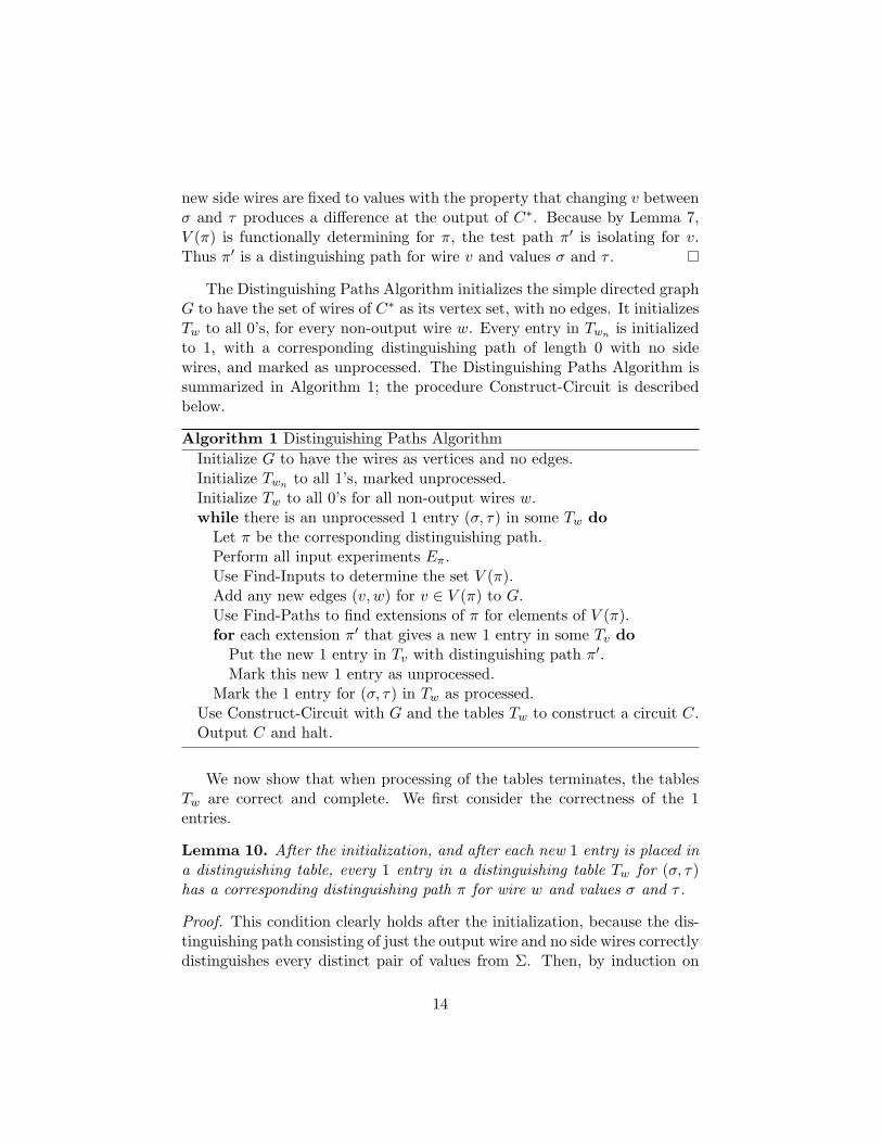
The Distinguishing Paths Algorithm initializes the simple directed graphG to have the set of wires of C∗ as its vertex set, with no edges. It initializesTw to all 0’s, for every non-output wire w. Every entry in Twn is initializedto 1, with a corresponding distinguishing path of length 0 with no sidewires, and marked as unprocessed. The Distinguishing Paths Algorithm issummarized in Algorithm 1; the procedure Construct-Circuit is describedbelow.

Algorithm 1 Distinguishing Paths AlgorithmInitialize G to have the wires as vertices and no edges.Initialize Twn to all 1’s, marked unprocessed.Initialize Tw to all 0’s for all non-output wires w.while there is an unprocessed 1 entry (σ, τ) in some Tw do

Let π be the corresponding distinguishing path.Perform all input experiments Eπ.Use Find-Inputs to determine the set V (π).Add any new edges (v, w) for v ∈ V (π) to G.Use Find-Paths to find extensions of π for elements of V (π).for each extension π′ that gives a new 1 entry in some Tv do

Put the new 1 entry in Tv with distinguishing path π′.Mark this new 1 entry as unprocessed.

Mark the 1 entry for (σ, τ) in Tw as processed.Use Construct-Circuit with G and the tables Tw to construct a circuit C.Output C and halt.

We now show that when processing of the tables terminates, the tablesTw are correct and complete. We first consider the correctness of the 1entries.

Lemma 10. After the initialization, and after each new 1 entry is placed ina distinguishing table, every 1 entry in a distinguishing table Tw for (σ, τ)has a corresponding distinguishing path π for wire w and values σ and τ .

Proof. This condition clearly holds after the initialization, because the dis-tinguishing path consisting of just the output wire and no side wires correctlydistinguishes every distinct pair of values from Σ. Then, by induction on

14

the number of new 1 entries in distinguishing path tables, when an existing1 entry in Tw gives rise to a new one in Tv, then the path π from Tw isa correct distinguishing path for w. Thus, by Lemma 8, the Find-Inputsprocedure correctly finds the set V (π) of inputs of w relevant with respectto π, and by Lemma 9, the Find-Paths procedure correctly finds extensionsof π to distinguishing paths π′ for elements of V (π). Thus, any new 1 entryin a table Tv will have a correct corresponding distinguishing path.

A distinguishing table Tw is complete if for every pair of values σ, τ ∈ Σsuch that σ and τ are distinguishable for w, Tw has a 1 entry for (σ, τ).

Lemma 11. When the Distinguishing Paths Algorithm terminates, Tw iscomplete for every wire w in C∗.

Proof. Assume to the contrary and look at a wire w at the smallest possibledepth such that Tw is incomplete; assume it lacks a 1 entry for the pair (σ, τ),which are distinguishable for w. Note that w cannot be the output wire.Because the depth of w is at least one more than the depth of any descendantof w, all wires on all directed paths from w to the root have completedistinguishing tables. By Lemma 10, all the entries in all distinguishingtables are also correct.

Because σ and τ are distinguishable for w, by Lemma 3 there exists adistinguishing path π for wire w and values σ and τ . On this distinguishingpath, w is followed by some wire x. The wires along π starting with x andomitting any side wires that are inputs of x is a distinguishing path for wirex and values σ′ and τ ′, where σ′ is the value that x takes when w = σ andτ ′ is the value that x takes when w = τ in any experiment agreeing with π.

Because x is a descendant of w, its distinguishing table Tx is completeand correct. Thus, there exists in Tx a 1 entry for (σ′, τ ′) and a corre-sponding distinguishing path πx. This 1 entry must be processed beforethe Distinguishing Paths Algorithm terminates. When it is processed, twoof the input experiments for πx will set the inputs of x in agreement withπ, and set w to σ and τ respectively. Thus, w will be discovered to be arelevant input of x with respect to π, and a distinguishing experiment forwire w and values σ and τ will be found, contradicting the assumption thatTw never gets a 1 entry for (σ, τ). Thus, no such wire w can exist and allthe distinguishing tables are complete.

Construct-Circuit. Now we show how to construct a circuit C behav-iorally equivalent to C∗ given the graph G and the final distinguishing tables.G is the graph of C, determining the input relation between wires. Note

15

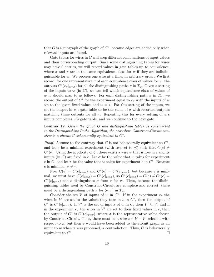
that G is a subgraph of the graph of C∗, because edges are added only whenrelevant inputs are found.

Gate tables for wires in C will keep different combinations of input valuesand their corresponding output. Since some distinguishing tables for wiresmay have 0 entries, we will record values in gate tables up to equivalence,where σ and τ are in the same equivalence class for w if they are indistin-guishable for w. We process one wire at a time, in arbitrary order. We firstrecord, for one representative σ of each equivalence class of values for w, theoutputs C∗(eπ|w=σ) for all the distinguishing paths π in Tw. Given a settingof the inputs to w (in C), we can tell which equivalence class of values ofw it should map to as follows. For each distinguishing path π in Tw, werecord the output of C∗ for the experiment equal to eπ with the inputs of wset to the given fixed values and w = ∗. For this setting of the inputs, weset the output in w’s gate table to be the value of σ with recorded outputsmatching these outputs for all π. Repeating this for every setting of w’sinputs completes w’s gate table, and we continue to the next gate.

Lemma 12. Given the graph G and distinguishing tables as constructedin the Distinguishing Paths Algorithm, the procedure Construct-Circuit con-structs a circuit C behaviorally equivalent to C∗.

Proof. Assume to the contrary that C is not behaviorally equivalent to C∗,and let e be a minimal experiment (with respect to �) such that C(e) 6=C∗(e). Using the acyclicity of C, there exists a wire w that is free in e and itsinputs (in C) are fixed in e. Let σ be the value that w takes for experimente in C, and let τ be the value that w takes for experiment e in C∗. Becausee is minimal, σ 6= τ .

Now C(e) = C(e|w=σ) and C∗(e) = C∗(e|w=τ ), but because e is mini-mal, we must have C(e|w=σ) = C∗(e|w=σ), so C∗(e|w=σ) = C(e) 6= C∗(e) =C∗(e|w=τ ) and e distinguishes σ from τ for w. Thus, because the distin-guishing tables used by Construct-Circuit are complete and correct, theremust be a distinguishing path π for (σ, τ) in Tw.

Consider the set V of inputs of w in C∗. If in the experiment eπ thewires in V are set to the values they take in e in C∗, then the output ofC∗ is C∗(e|w=τ ). If V ′ is the set of inputs of w in C, then V ′ ⊆ V , and ifin the experiment eπ the wires in V ′ are set to their fixed values in e, thenthe output of C∗ is C∗(e|w=σ), where σ is the representative value chosenby Construct-Circuit. Thus, there must be a wire v ∈ V − V ′ relevant withrespect to π, but then v would have been added to the circuit graph as aninput to w when π was processed, a contradiction. Thus, C is behaviorallyequivalent to C∗.

16

We analyze the total number of value injection queries used by the Dis-tinguishing Paths Algorithm; the running time is polynomial in the numberof queries. To construct the distinguishing tables, each 1 entry in a distin-guishing table is processed once. The total number of possible 1 entries inall the tables is bounded by ns2. The processing for each 1 entry is to takethe corresponding distinguishing path π and construct the set Eπ of inputexperiments, each of which consists of choosing up to 2k wires and settingthem to arbitrary values from Σ, for a total of O(n2ks2k) queries to con-struct Eπ. Thus, a total of O(n2k+1s2k+2) value injection queries are usedto construct the distinguishing tables.

To build the gate tables, for each of n wires, we try at most s2 distin-guishing path experiments for at most s values of the wire, which takes atmost s3 queries. We then run the same experiments for each possible set-ting of the inputs to the wire, which takes at most sks2 experiments. ThusConstruct-Circuit requires a total of O(n(s3 + sk+2)) experiments, whichare already among the ones made in constructing the distinguishing tables.Note that every experiment fixes at most O(kd) wires, where d is the depthof C∗. This concludes the proof of Theorem 5.

4 Circuits with Bounded Shortcut Width

In this section we describe the Shortcuts Algorithm, which generalizes theDistinguishing Paths Algorithm to circuits with bounded shortcut width asfollows.

Theorem 13. The Shortcuts Algorithm learns the class of circuits havingn wires, alphabet size s, fan-in bound k, and shortcut width bounded by busing a number of value injection queries bounded by (ns)O(k+b) and timepolynomial in the number of queries.

When C∗ is not transitively reduced, there may be edges of its graphthat are important to the behavior of the circuit, but are not completelydetermined by the behavior of the circuit. For example, the three circuitsgiven in Figure 1 of [7] are behaviorally equivalent, but have different graphs;a behaviorally correct circuit cannot be constructed with just the edges thatare common to the three circuit graphs. Thus, the Shortcuts Algorithmfocuses on finding a sufficient set of experiments for C∗, and uses CircuitBuilder [7] to build the output circuit C.

A gate with gate function g and input wires u1, . . . , u` is wrong for win C∗ if there exists an experiment e in which the wires u1, . . . , u` are fixed,

17

say to values uj = σj , and w is free, and there is an experiment e such thatC∗(e) 6= C∗(e|w=g(σ1,...,σ`)), and is correct otherwise. The experiment e,which we term a witness experiment for this gate and wire, shows thatno circuit C using this gate for w can be behaviorally equivalent to C∗.A set E of experiments is sufficient for C∗ if for every wire w and everycandidate gate that is wrong for w, E contains a witness experiment for thisgate and this wire.

Lemma 14. [7] If the input E to Circuit Builder is a sufficient set of exper-iments for C∗, then the circuit C that it outputs is behaviorally equivalentto C∗.

The need to guarantee witness experiments for all possible wrong gatesmeans that the Shortcuts Algorithm will learn a set of distinguishing tablesfor the restriction of C∗ obtained by fixing u1, . . . , u` to values σ1, . . . , σ` forevery choice of at most k wires uj and every choice of assignments of fixedvalues to them.

On the positive side, we can learn quite a bit about the topology of acircuit C∗ from its behavior. An edge (v, w) of the graph of C∗ is discover-able if it is the initial edge on some minimal distinguishing experiment e forv and some values σ1 and σ2. This is a behaviorally determined property;all circuits behaviorally equivalent to C∗ must contain all the discoverableedges of C∗.

Because e is minimal, w must take on two different values, say τ1 andτ2 in e|v=σ1 and e|v=σ2 respectively.. Moreover, e|v=σ1 must be a minimalexperiment distinguishing τ1 from τ2 for w; this purely behavioral propertyis both necessary and sufficient for a pair (v, w) to be a discoverable edge.

Lemma 15. The pair (v, w) is a discoverable edge of C∗ if and only if thereis an experiment e and values σ1, σ2, τ1, τ2 such that e is a minimal exper-iment distinguishing σ1 from σ2 for v, and e|v=σ1 is a minimal experimentdistinguishing τ1 from τ2 for w.

We now generalize the concept of distinguishing paths to leave potentialshortcut wires unassigned. Assume that C∗ is a circuit, with n wires, analphabet Σ of s symbols, fan-in bound k, and shortcut width bound b. Atest path with shortcuts π is a directed path of wires from some wirew to the output, a set S of side wires assigned fixed values from Σ, anda set K of cut wires such that S and K are disjoint and neither containsw, and each wire in S ∪K is an input to at least one wire beyond w in thedirected path of wires. One intuition for this is that the wires in K could

18

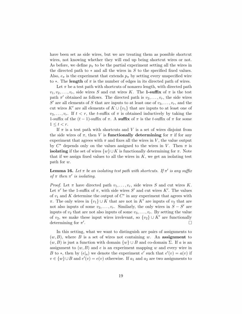
have been set as side wires, but we are treating them as possible shortcutwires, not knowing whether they will end up being shortcut wires or not.As before, we define pπ to be the partial experiment setting all the wires inthe directed path to ∗ and all the wires in S to the specified fixed values.Also, eπ is the experiment that extends pπ by setting every unspecified wireto ∗. The length of π is the number of edges in its directed path of wires.

Let π be a test path with shortcuts of nonzero length, with directed pathv1, v2, . . . , vr, side wires S and cut wires K. The 1-suffix of π is the testpath π′ obtained as follows. The directed path is v2, . . . , vr, the side wiresS′ are all elements of S that are inputs to at least one of v3, . . . , vr, and thecut wires K ′ are all elements of K ∪ {v1} that are inputs to at least one ofv3, . . . , vr. If t < r, the t-suffix of π is obtained inductively by taking the1-suffix of the (t− 1)-suffix of π. A suffix of π is the t-suffix of π for some1 ≤ t < r.

If π is a test path with shortcuts and V is a set of wires disjoint fromthe side wires of π, then V is functionally determining for π if for anyexperiment that agrees with π and fixes all the wires in V , the value outputby C∗ depends only on the values assigned to the wires in V . Then π isisolating if the set of wires {w}∪K is functionally determining for π. Notethat if we assign fixed values to all the wires in K, we get an isolating testpath for w.

Lemma 16. Let π be an isolating test path with shortcuts. If π′ is any suffixof π then π′ is isolating.

Proof. Let π have directed path v1, . . . , vr, side wires S and cut wires K.Let π′ be the 1-suffix of π, with side wires S′ and cut wires K ′. The valuesof v1 and K determine the output of C∗ in any experiment that agrees withπ. The only wires in {v1} ∪K that are not in K ′ are inputs of v2 that arenot also inputs of some v3, . . . , vr. Similarly, the only wires in S − S′ areinputs of v2 that are not also inputs of some v3, . . . , vr. By setting the valueof v2, we make these input wires irrelevant, so {v2} ∪ K ′ are functionallydetermining for π′.

In this setting, what we want to distinguish are pairs of assignments to(w,B), where B is a set of wires not containing w. An assignment to(w,B) is just a function with domain {w} ∪B and co-domain Σ. If a is anassignment to (w,B) and e is an experiment mapping w and every wire inB to ∗, then by (e|a) we denote the experiment e′ such that e′(v) = a(v) ifv ∈ {w}∪B and e′(v) = e(v) otherwise. If a1 and a2 are two assignments to

19

(w,B), then the experiment e distinguishes a1 from a2 if e maps {w} ∪Bto ∗ and C∗(e|a1) 6= C∗(e|a2).

Let π be a distinguishing path with shortcuts with initial path wirew, side wires S and cut wires K. Then π is distinguishing for the pair(w,B) and assignments a1 and a2 to (w,B) if K ⊆ B, B ∩ S = ∅, π isisolating and eπ distinguishes a1 from a2. If such a path exists, we say(w,B) is distinguishable for a1 and a2. Note that this condition requiresthat π not set any of the wires in B. When B = ∅, these definitions reduceto the previous ones.

4.1 The Shortcuts Algorithm

Overview of algorithm. We assume that at most k wires u1, . . . , u` havebeen fixed to values σ1, . . . , σ`, and denote by C∗ the resulting circuit. Theprocess described is repeated for every choice of wires and values. Like theDistinguishing Paths Algorithm, the Shortcuts Algorithm builds a directedgraph G whose vertices are the wires of C∗, in which an edge (v, w) is addedwhen v is discovered to be an input to w in C∗; one aim of the algorithm isto find all the discoverable edges of C∗.

Distinguishing tables. The Shortcuts Algorithm maintains a distinguish-ing table Tw for each wire w. Each entry in Tw is indexed by a triple,(B, a1, a2), where B is a set of at most b wires not containing w, and a1

and a2 are assignments to (w,B). If an entry exists for index (B, a1, a2),it contains π, a distinguishing path with shortcuts that is distinguishingfor (w,B), a1 and a2. The entry also contains a bit marking the entry asprocessed or unprocessed.

Initialization. The distinguishing table Twn for the output wire is ini-tialized with entries indexed by (∅, {wn = σ}, {wn = τ}) for every pair ofdistinct symbols σ, τ ∈ Σ, each containing the distinguishing path of length0 with no side wires and no cut wires. Each such entry is marked as unpro-cessed. All other distinguishing tables are initialized to be empty.

While there is an entry in some distinguishing table Tw marked as un-processed, say with index (B, a1, a2) and π the corresponding distinguishingpath with shortcuts, the Shortcuts Algorithm processes it and marks it asprocessed. To process it, the algorithm first uses the entry try to discoverany new edges (v, w) to add to the graph G; if a new edge is added, allof the existing entries in the distinguishing table for wire w are marked asunprocessed. Then the algorithm attempts to find new distinguishing paths

20

with shortcuts obtained by extending π in all possible ways. If an extensionis found to a test path with shortcuts π′ that is distinguishing for (w′, B′), a′1and a′2, if there is not already an entry for (B′, a′1, a

′2), or, if π′ is of shorter

length that the existing entry for (B′, a′1, a′2), then its entry is updated to π′

and marked as unprocessed. When all possible extensions have been tried,the algorithm marks the entry in Tw for (B, a1, a2) as processed.

In contrast to the case of the Distinguishing Paths Algorithm, the Short-cuts Algorithm tries to find a shortest distinguishing path with shortcutsfor each entry in the table. When no more entries marked as unprocessedremain in any distinguishing table, the algorithm constructs a set of ex-periments E as described below, calls Circuit Builder on E, outputs theresulting circuit C, and halts.

Processing an entry. Let (B, a1, a2) be the index of an unprocessed entryin a distinguishing table Tw, with corresponding distinguishing path withshortcuts, π, where the side wires of π are S and the cut wires are K. Notethat K ⊆ B and S ∩B = ∅. Let the set Eπ consist of every experiment thatagrees with π, arbitrarily fixes the wires in K, and arbitrarily fixes up to 2kadditional wires not in K and not set by pπ, and sets the remaining wiresfree. There are O((ns)2ksb) experiments in Eπ; the algorithm makes a valueinjection query for each of them.

Finding relevant inputs. For every assignment a of fixed values to K,the resulting path πa is an isolating test path for w. We use the Find-Inputsprocedure (in Section 3.3) to find relevant inputs to w with respect to πa,and let V ∗(π) be the union of the sets of wires returned by Find-Inputs overall assignments a to K. For each v ∈ V ∗(π), add the edge (v, w) to G if itis not already present, and mark all existing entries in all the distinguishingtables for wire w as unprocessed.

Lemma 17. The wires in V ∗(π) are inputs to w and the wires in V ∗(π)∪Kare functionally determining for π.

Proof. This follows from Lemma 8, because for each assignment a to K, theresulting πa is an isolating path for w, and any wires in the set returned byFind-Inputs are indeed inputs to w. Also, for each assignment a to K, theset V (πa) is functionally determining for πa, and is contained in V ∗(π).

Additional input test. The Shortcuts Algorithm makes an additionalinput test if π distinguishes two assignments a1 and a2 such that there is

21

a wire w′ ∈ K such that a1 and a2 agree on every wire other than w.Let π′ be the distinguishing path obtained from π by fixing every wire inK − {w} to its value in a1. If there is an experiment e agreeing with π′

and setting w to ∗ and fixing every element of V (π′), and two values σ1

and σ2 such that C∗(e|v=σ1) 6= C∗(e|v=σ2), and, moreover, for every τ ∈ Σ,C∗(e|w=τ,v=σ1) = C∗(e|w=τ,v=σ2), then add edge (v, w) to G if it is notalready present, and mark all the existing entries in the distinguishing tablefor wire w as unprocessed.

Lemma 18. If edge (v, w) is added to G by this additional input test, thenv is an input of w in C∗.

Proof. Note that w must take two different values, say τ1 and τ2, in theexperiments e|v=σ1 and e|v=σ2 ; thus, w must be a descendant of v. Moreover,C∗(e|w=τ1,v=σ1) = C∗(e|w=τ1,v=σ2) and C∗(e|w=τ2,v=σ1) = C∗(e|w=τ2,v=σ2),from which we conclude that C∗(e|w=τ1,v=σ1) 6= C∗(e|w=τ2,v=σ1).

If v is not an input of w, then let U be the set of all inputs of w. Ine, if we set v = σ1 and w = ∗ and the wires in U as induced by e|v=σ1 ,then w = τ1 and the output of C∗ is C∗(e|w=τ1,v=σ1). If we then change thevalues on wires in U one by one to their values in e|v=σ2 , because the finalresult have w = τ2 and output C∗(e|v=σ1,w=τ2), there must be an input usuch that fixing the other inputs to w and changing u’s value changes theoutput with respect to e|v=σ1 . Thus, u is a relevant input with respect tothe distinguishing path π{v=σ1}, and must be in the set V (π). This is acontradiction, because wires in V (π) are fixed in e, and u must change valuefrom e|v=σ1 and e|v=σ2 . Thus v must be an input of w.

Extending a distinguishing path. After finding as many inputs of w aspossible using π, the Shortcuts Algorithm attempts to extend π as follows.Let IG(w) be the set of all inputs of w in G. For each pair (w′,K ′) suchthat w′ ∈ IG(w) and K ′ is a set of at most b wires not containing w′ suchthat K ′ ⊆ IG(w) ∪K and K ′ is disjoint from the path wires and side wiresof π, we let S0 = (K ∪ V ∗(π)) − ({w′} ∪K ′). Note that the set of wires inS0 ∪K ′ ∪ {w′} is functionally determining for π.

For each assignment a of fixed values to S0, the algorithm extends π toπ′ as follows. It adds w′ to the start of the directed path, adds S0 to theset of side wires (fixed to the values assigned by a) and takes the cut wiresto be K ′. Note that every wire in K ′ is an input to some wire beyond w onthe path. Because w′ is an input of w, and all of the wires in V ∗(π)∪K areaccounted for among (w,K ′) and S′, and all of the wires in S′ are inputs to

22

w or wires beyond w on the path, the result is an isolating test path withshortcuts for (w′,K ′).

The algorithm then searches through all triples (B′, a′1, a′2) where B′ is

a set of at most b wires not containing w′, and a′1 and a′2 are assignments to(w′, B′), to discover whether π′ is distinguishing for (w′, B′), a′1 and a′2. Ifso, the algorithm checks the distinguishing table Tw′ and creates or updatesthe entry for index (B′, a′1, a

′2) as follows. If there is no such entry, one is

created with π′. If there already is an entry and π′ is shorter than the pathin the entry, then the entry is changed to contain π′. If the entry is createdor changed by this operation, it is marked as unprocessed. When all possibleextensions of π have been tried, the entry in Tw for (B, a1, a2) is marked asprocessed.

Correctness and completeness. We define the distinguishing table Twto be correct if whenever π is an entry in Tw for (B, a1, a2), then π is adistinguishing path with shortcuts that is distinguishing for (w,B), a1 anda2. For each wire w, let B(w) denote the set of shortcut wires of w in thetarget circuit C∗. If π is a distinguishing path with shortcuts such that everyedge in its directed path is discoverable, we say that π is discoverable.The distinguishing Tw table is complete if for every pair a1 and a2 ofassignments to (w,B(w)) that are distinguishable by a discoverable path,there is an entry in Tw for index (B(w), a1, a2).

Lemma 19. When Shortcuts Algorithm finishes the processing of the dis-tinguishing tables, every distinguishing table Tw is correct and complete.

Proof. The correctness follows inductively from the correctness of the ini-tialization of Twn by the arguments given above. To prove completeness, weprove the following stronger condition about the distinguishing tables whenthe Shortcuts Algorithm finishes processing them: (1) for every wire w andevery pair a1 and a2 of assignments to (w,B(w)) that are distinguishableby a discoverable path, the entry for (B(w), a1, a2) is a shortest discoverabledistinguishing path with shortcuts that is distinguishing for (w,B(w)), a1

and a2.Condition (1) clearly holds for Twn after it is initialized, and this table

does not change thereafter. Assume to the contrary that condition (1) doesnot hold and let w be a wire of the smallest possible depth such that Twdoes not satisfy condition (1). Note that w is not the output wire.

There must be assignments a1 and a2 for (w,B(w)) that are distinguish-able by a discoverable path such that in Tw, the entry for (B(w), a1, a2)

23

is either nonexistent or not as short as possible. Let π be a shortest pos-sible discoverable distinguishing path with shortcuts that is distinguishingfor (w,B(w)), a1 and a2. Let S be the side wires of π, with assignment a,and let K be the cut wires of π. Then we have K ⊆ B and S ∩ B = ∅.Because w is not the output wire, the directed path in π is of length at least1. Let π′ be the 1-suffix of π, with initial vertex w′, side wires S′ and cutwires K ′. Note that (w,w′) must be a discoverable edge and that π′ is alsodiscoverable. By Lemma 16, π′ is isolating.

For any two assignments a′1 and a′2 to (w′, B(w′)) such that a′j(u) is thevalue of u in eπ|aj for each u ∈ {w′} ∪K ′, we have that π′ is distinguishingfor (w′, B(w′)), a′1 and a′2. To see this, note that {w′} ∪K ′ is functionallydetermining for π′, so C∗(eπ′ |a′j ) = C∗(eπ|aj ) for j = 1, 2, and these lattertwo values are distinct. Let a′j denote the assignment to (w′, B(w′)) inducedby the experiment eπ|aj for j = 1, 2; these two assignments have the requiredproperty.

Because the depth of w′ is smaller than the depth of w, condition (1)must hold for Tw′ , and the distinguishing table for Tw′ must contain anentry for (B(w′), a′1, a

′2) that is a shortest discoverable distinguishing path

with shortcuts π′′ that is distinguishing for B(w′), a′1 and a′2. Note that thelength of π′′ is at most the length of π minus 1.

We argue that the discoverable edge (w,w′) must be added to G by theShortcuts Algorithm. This edge is the first edge on a minimal experiment edistinguishing σ1 from σ2 for w. This corresponds to a distinguishing pathρ with no cut edges distinguishing σ1 from σ2 for w, and every edge of thispath is also discoverable. There are two cases, depending on whether w is ashortcut of w′ on the path or not.

If w is not a shortcut edge of w′ on the path, then the 1-suffix of ρ will bea discoverable distinguishing path with no cut edges that is distinguishingfor w′, τ1, and τ2, where these are the values w′ takes in e|w=σj for j = 1, 2.Because condition (1) holds for Tw′ , there will be an entry in Tw′ containinga distinguishing path with shortcuts for (w′, B(w′)) that distinguishes thetwo assignments that set B(w′) as in e and set w′ to τ1 and τ2. Because wis a relevant input with respect to ρ, the edge (w,w′) will be added to G ifit is not already present when ρ is processed.

If w is a shortcut edge of w′ on the path, then the 1-suffix of ρ will bea discoverable distinguishing path with cut edges {w} that is distinguishingfor the assignments α1 = {w = σ1, w

′ = τ1} and α2 = {w = σ2, w′ = τ2}.

Because w ∈ B(w′) and Tw′ satisfies condition (1), there will be an entry ρin Tw′ for (w′, B(w′)) that distinguishes the two assignments to (w′, B(w′))

24

that agree with α1 and α2 on w′ and w, and set every other element of B(w′)as in e. When the entry ρ is processed, the additional input test will discoverthe edge (w,w′) and add it to the graph G if it is not already present. In fact,this shows that every discoverable edge (v, w′) will eventually be discoveredby the algorithm because Tw′ is complete.

Thus, we can be sure that the entry π′′ will be (re)processed when everydiscoverable edge (v, w′) is present in G, including (w,w′). When this hap-pens, the entry π′′ will be extended to a distinguishing path with shortcutsthat is distinguishing for (w,B(w)), a1 and a2 and has length at most thatof π. To see that this holds, note that if v is a side wire of π′′, then it cannotbe an ancestor of w′ because otherwise it is a shortcut wire of w′ and inB(w′), which is disjoint from the side wires of π′′. Thus, the side wires of π′′

cannot include any input of w′ or any wire in B(w), because all these wiresare ancestors of w′. Moreover, since all the discoverable inputs to w′ havebeen added to G, one of the possible extensions of π′′ will set (some of) theinputs of w′ in such a way that moving from assignment a1 to assignmenta2 to (w,B(w)) with the other side gate settings of π′′ will move from a′1 toa′2 for (w′, B(w′)),

Thus, the entry (B, a1, a2) will exist and be of length at most the lengthof π when the algorithm finishes processing the distinguishing tables. Thiscontradiction shows that all the distinguishing tables must be complete.

Building a circuit. When all the entries in all the distinguishing tablesare marked as processed, the Shortcuts Algorithm constructs a set E of ex-periments. For every table Tw and every distinguishing path π for (B, a1, a2)in the table such that a1(u) = a2(u) for every u ∈ B, and every set V ofat most k wires not set by pπ and every assignment a to V , add to E theexperiment eπ|a, that extends eπ by the assignment a. After iterating theabove process over all possible choices of at most k wires u1, . . . , u` and as-signments to them, the algorithm takes the union of all the resulting sets ofexperiments E and calls Circuit Builder [7] on this union and outputs thereturned circuit C and halts.

Lemma 20. The circuit C is behaviorally equivalent to the target circuitC∗.

Proof. We show that the completeness of the distinguishing tables impliesthat the set E of experiments is sufficient, and apply Lemma 14 to concludethat C is behaviorally equivalent to C∗. Suppose a gate g with inputs

25

u1, . . . , u` is wrong for wire w in C∗. Then there exists a minimal experimente that witnesses this; e fixes all the wires u1, . . . , u`, say as uj = σj forj = 1, . . . , `, sets the wire w free and is such that C∗(e) 6= C∗(e|w=g(σ1,...,σ`

)).Consider the iteration of the table-building process for the circuit C∗

with the restriction uj = σj for j = 1, . . . , `. In this circuit, e distinguishesbetween w = σ and w = τ , where σ is the value w takes in C∗ for e,and τ = g(σ1, . . . , σ`). Note that the free wires of e form a directed pathof discoverable edges. Because the table Tw is complete, there will be adistinguishing path π with shortcuts for (w,B(w)) for assignments a1 anda2 where a1(w) = σ and a2(w) = τ , and a1(v) = a2(v) for all v ∈ B(w).For every input v of w in C∗ that is not among u1, . . . , u`, π does not setv, because it only sets wires that are inputs to descendants of w, and anyinput of w that is an input of a descendant of w is a short cut wire of wand therefore in B(w). However, π does not set any wires in B(w). Thus,among the choices of sets of at most k wires and values to set them to, therewill be one that sets just the inputs (in C∗) of w as in e. The correspondingexperiment e′ in E will be a witness experiment eliminating the gate g withinputs u1, . . . , u`, so the set of experiments to Circuit Builder is sufficientfor C∗.

Running time. To analyze the running time of the Shortcuts Algorithm,note that there are O(nksk) choices of at most k wires and values fromΣ to fix them to; this bounds the number of iterations of the table build-ing process. In each iteration, there are O(nb+1s2b+2) total entries in thedistinguishing tables. Each entry in a distinguishing table may be pro-cessed several times: when it first appears in the table, and each time itsdistinguishing path is replaced by a shorter one, and each time a new in-put of w is discovered, for a total of at most n + k times. Thus, the to-tal number of entry-processing events by the algorithm in one iteration isO((n + k)nb+1s2b+2). Each such event makes O((ns)2ksb) value injectionqueries, so O((n + k)n2k+b+1s2k+3b+2) value injection queries are made bythe algorithm in each iteration, for a total of O((n + k)n3k+b+1s3k+3b+2)value injection queries made by the Shortcuts Algorithm. The number ofexperiments given as input to Circuit Builder is O(n2k+b+1s2k+2b+2), be-cause each final entry may give rise to at most O(nksk) experiments in E ineach iteration. This concludes the proof of Theorem 13.

26

5 Learning Analog Circuits via Discretization

We first give a simple example of an analog circuit. We then show how toconstruct a discrete approximation of an analog circuit, assuming its gatefunctions satisfy a Lipschitz condition with constant L, and apply the large-alphabet learning algorithm of Theorem 13, to get a polynomial-time algo-rithm for approximately learning an analog circuit with logarithmic depth,bounded fan-in and bounded shortcut width.

5.1 Example of an analog circuit

For example, let ∧(x, y) = xy for all x, y ∈ [0, 1] and let ∨(x, y) = x+y−xyfor all x, y ∈ [0, 1]. (Note that these are polynomial representations ofconjunction and disjunction when restricted to the values 0 and 1.) Then ∧and ∨ are analog functions of arity 2, and we define a circuit with 6 wires asfollows. Let g1 be the constant function 0.1, g2 be the constant function 0.6and g3 be the constant function 0.8. These functions assign default values tothe corresponding wires. Let g4 be the function ∨, and let its pair of inputsbe w1, w2. Let g5 be the function ∨, and let its pair of inputs be w2, w3.Finally, let w6 be the function ∧, and let its pair of inputs be w4, w5. Ifwe consider the experiment e0 that assigns ∗ to every wire, we calculate thevalues wi(e0) as follows. Using their default values,

w1(e0) = 0.1, w2(e0) = 0.6, w3(e0) = 0.8.

Then, because the inputs to w4 and w5 have defined values,

w4(e0) = ∨(0.1, 0.6) = 0.64, w5(e0) = ∨(0.6, 0.8) = 0.92.

Because the inputs to w6 now have defined values,

w6 = ∧(0.64, 0.92) = 0.5888.

If we consider the experiment e1 that fixes the value of w5 to 0.2 and assigns∗ to every other wire, then as before,

w1(e1) = 0.1, w2(e1) = 0.6, w3(e1) = 0.8, w4(e1) = 0.64.

However, because the value of w5 is fixed to 0.2 in e1,

w5(e1) = 0.2, w6(e1) = ∧(0.64, 0.2) = 0.128.

27

5.2 A Lipschitz condition

An analog function g of arity k satisfies a Lipschitz condition with constantL if for all x1, . . . , xk and x′1, . . . , x

′k from [0, 1] we have

|g(x1, . . . , xk)− g(x′1, . . . , x′k)| ≤ Lmax

i|xi − x′i|.

For example, the function ∧(x, y) = xy satisfies a Lipschitz condition withconstant 2. A Lipschitz condition on an analog function allows us to boundthe error of a discrete approximation to the function. For more on Lipschitzconditions, see [14].

Let m be a positive integer. We define a discretization function Dm from[0, 1] to the m points {1/2m, 3/2m, . . . , (2m− 1)/2m} by mapping x to theclosest point in this set (choosing the smaller point if x is equidistant fromtwo of them.) Then |x −Dm(x)| ≤ 1/2m for all x ∈ [0, 1]. We extend Dm

to discretize analog experiments e by defining Dm(∗) = ∗ and applying itcomponentwise to e. An easy consequence is the following.

Lemma 21. If g is an analog function of arity k, satisfying a Lipschitzcondition with constant L and m is a positive integer, then for all x1, . . . , xkin [0, 1], |g(x1, . . . , xk)− g(Dm(x1), . . . , Dm(xk))| ≤ L/2m.

5.3 Discretizing analog circuits

We describe a discretization of an analog gate function in which the inputsand the output may be discretized differently. Let g be an analog functionof arity k and r, s be positive integers. The (r, s)-discretization of g is g′,defined by

g′(x1, . . . , xk) = Dr(g(Ds(x1), . . . , Ds(xk))).

Let C be an analog circuit of depth dmax and let L and N be positiveintegers. Define md = N(3L)d for all nonnegative integers d. We constructa particular discretization C ′ of C by replacing each gate function gi byits (md,md+1)-discretization, where d is the depth of wire wi. We alsoreplace the value set Σ = [0, 1] by the value set Σ′ equal to the union ofthe ranges of Dmd

for 0 ≤ d ≤ dmax. Note that the wires and tuples ofinputs remain unchanged. The resulting discrete circuit C ′ is termed the(L,N)-discretization of C.

Lemma 22. Let L and N be positive integers. Let C be an analog cir-cuit of depth dmax whose gate functions all satisfy a Lipschitz conditionwith constant L. Let C ′ denote the (L,N)-discretization of C and let M =N(3L)dmax. Then for any experiment e for C, |C(e)− C ′(DM (e))| ≤ 1/N.

28

Proof. Define md = N(3L)d for all nonnegative integers d; then M = mdmax .We prove the stronger condition that for every experiment e for C and everywire wi, if d is the depth of wi, we have

|wi(e)− w′i(DM (e))| ≤ 1/md,

where wi(e) is the value of wire wi in C for experiment e and w′i(DM (e)) isthe value of wire wi in C ′ for experiment DM (e). Because the output wireis at depth d = 0, this will imply that C(e) and C ′(DM (e)) do not differ bymore than 1/N .

Let e be an arbitrary experiment for C. We proceed by downward in-duction on the depth d of wi. When this quantity is dmax, the wire wi is atmaximum depth and has no inputs. The wire wi is fixed in e if and only ifit is fixed in DM (e), and in either case, the values assigned to wi agree towithin 1/2M < 1/mdmax . Now consider wi at depth d, assuming inductivelythat the condition holds for all wires at greater depth. If wi is fixed in e thenit is fixed in DM (e) and the values assigned to it differ by at most 1/2M .If wi is free in e then it is free in DM (e). Consider the input wires to wi,say wj1 , . . . , wjs ; these are all at depth at least d + 1, so by the inductivehypothesis

|wjr(e)− w′jr(DM (e))| ≤ 1/md+1,

for r = 1, . . . , s.Note that

wi(e) = gi(wj1(e), . . . , wjs(e))

andw′i(DM (e)) = Dmd

(gi(y1, . . . , ys)),

where yr = Dmd+1(w′jr(DM (e))) for r = 1, . . . , s. Note that by the properties

of the discretization function,

|yr − w′jr(DM (e))| ≤ 1/(2md+1).

By the Lipschitz condition on the gate function gi we have

|gi(wj1(e), . . . , wjs(e))− gi(y1, . . . , ys)| ≤ L(3/2)(1/md+1) = 1/(2md),

because|wjr(e)− yr| ≤ 1/md+1 + 1/(2md+1).

Discretizing the output of gi by Dmdadds at most 1/(2md) to the difference,

so|gi(wj1(e), . . . , wjs(e))−Dmd

(gi(y1, . . . , yx))| ≤ 1/md,

29

that is,|wi(e)− w′i(DM (e))| ≤ 1/md,

which completes the induction.

This lemma shows that if every gate of C satisfies a Lipschitz condi-tion with constant L, we can approximate C’s behavior to within ε usinga discretization with O((3L)d/ε) points, where d is the depth of C. Ford = O(log n), this bound is polynomial in n and 1/ε.

Theorem 23. There is a polynomial time algorithm that approximatelylearns any analog circuit of n wires, depth O(log n), constant fan-in, gatefunctions satisfying a Lipschitz condition with a constant bound, and short-cut width bounded by a constant.

6 Learning with Experiments and Counterexam-ples

In this section, we consider the problem of learning circuits using both valueinjection queries and counterexamples. In a counterexample query, thealgorithm proposes a hypothesis C and receives as answer either the factthat C exactly equivalent to the target circuit C∗, or a counterexample,that is, an experiment e such that C(e) 6= C∗(e). In [7], polynomial-timealgorithms are given that use value injection queries and counterexamplequeries to learn (1) acyclic circuits of arbitrary depth with arbitrary gatesof constant fan-in, and (2) acyclic circuits of arbitrary depth with AND,OR, NOT, NAND, and NOR gates of arbitrary fan-in.

The algorithm that we now develop generalizes both previous algorithmsby permitting any class of gates that is polynomial time learnable withcounterexamples. It also guarantees that the depth of the output circuitis no greater than the depth of the target circuit and that the number ofadditional wires fixed in value injection queries is bounded by O(kd), wherek is a bound on the fan-in and d is a bound on the depth of the targetcircuit.

An advantage of learning with counterexamples is its flexibility. As re-marked in [7], if the counterexample queries return counterexamples thatfix only the input wires of the circuit, learning algorithms output a circuitequivalent to the target circuit with respect to input/output behaviors. Ingeneral, the algorithms only output a circuit equivalent to the target withrespect to the set of counterexamples presented to them. Moreover, the

30

algorithms presented in this section can be naturally generalized to workwhen more than one gate is observable. In this case, an experiment e is acounterexample if C and C∗ compute one of the observable gates differentlyand the learning algorithm outputs a circuit that behaves the same way onall observable gates with respect to the given set of counterexamples.

6.1 The learning algorithm

The algorithm proceeds in a cycle of proposing a hypothesis, getting a coun-terexample, processing the counterexample, and then proposing a new hy-pothesis. Whenever we receive a counterexample e, we process the coun-terexample so that we can “blame” at least one gate; we find a witnessexperiment e∗ eliminating a candidate gate function g. In effect, we reducethe problem of learning a circuit to the problem of learning individual gateswith counterexamples.

An experiment e∗ is a witness experiment eliminating g, if and onlyif e∗ fixes all inputs of g but sets g free and C∗(e∗|w=g(e∗)) 6= C∗(e∗). It isimportant that we require e∗ fix all inputs of g, because then we know it isg and not its ancestors computing wrong values. The main operation of theprocedure that processes counterexamples is to fix wires to specific values.

Given a counterexample e, let procedure minimize fix wires in e whilepreserving the property that C(e) 6= C∗(e) until it cannot fix any more.Therefore, e∗ = minimize(e) is a minimal counterexample for C under thepartial order � defined in Sect. 2.2. The following lemma is a consequenceof Lemma 10 in [7].

Lemma 24. If e∗ is a minimal counterexample for C, there exists a gate gin C such that e∗ is a witness experiment for g.

Proof. Because C is acyclic, there exists a gate g that is free in e∗ such thatall the inputs of g are fixed in e∗. Then e∗ is a witness experiment for g, be-cause otherwise we have C∗(e∗|w=g(e∗)) = C∗(e∗) 6= C(e∗) = C(e∗|w=g(e∗)),which contradicts the minimality of e∗.

Although it does the job, the procedure minimize may fix many morewires than necessary. (In Section 6.2 we will describe a different algorithmthat will fix many fewer wires for certain classes of circuits.)

Now we run a separate counterexample learning algorithm for each in-dividual wire. Whenever C receives a counterexample, at least one of thelearning algorithms will receive one. However, if we run all the learningalgorithms simultaneously and let each learning algorithm propose a gate

31

function, the hypothesis circuit may not be acyclic. Instead we will use Al-gorithm 2 to coordinate them, which can be viewed as a generalization ofthe circuit building algorithm for learning AND/OR circuits in [7]. Conflictsare defined below.

Algorithm 2 Learning with experiments and counterexamplesRun an individual learning algorithm for each wire w. Each learningalgorithm takes as candidate inputs only wires that have fewer conflicts.Let C be the hypothesis circuit.while there is a counterexample for C do

Process the counterexample to obtain a counterexample for a wire w.Run the learning algorithm for w with the new counterexample.if there is a conflict for w then

Restart the learning algorithms for w and all wires whose candidateinputs have changed.

The algorithm builds an acyclic circuit C because each wire has as inputsonly wires that have fewer conflicts. At the start, each individual learningalgorithm runs with an empty candidate input set since there is yet no con-flict. Thus, each of them tries to learn each gate as a constant gate, andsome of them will not succeed. A conflict for w happens when there is nohypothesis in the hypothesis space that is consistent with the set of coun-terexamples received by w. For constant gates, there is a conflict when wereceive a counterexample for each of the s = |Σ| possible constant functions.We note that there will be no conflict for a wire w if the set of candidateinputs contains the set of true inputs of w in the target circuit C∗, becausethen the hypothesis space contains the true gate.

Whenever a conflict occurs for a wire, it has a chance of having morewires as candidate inputs. Therefore, our learning algorithm can be seen asrepeatedly rebuilding a partial order over wires based on their numbers ofconflicts. Another natural partial order on wires is given by the level of awire, defined as the length of a longest directed path from a constant gate tothe wire in the target circuit C∗. The following lemma shows an interestingconnection between levels and numbers of conflicts.

Lemma 25. The number of conflicts each wire receives is bounded above byits level.

Proof. A conflict happens to a wire w only when the candidate input wiresdo not contain all input wires of the true gate of w. Therefore, constantgates, whose levels are zero, have no conflict. Assuming the lemma is true

32

for all wires with level no higher than i, for a level i wire w, at the point whas i conflicts, all the input wires of w’s true gates have fewer conflicts thanw and thus are considered as candidate input wires for w by our algorithm.Therefore, w can not have more than i conflicts.

Corollary 26. The depth of C is at most the depth of C∗.

In fact, the depth of C is bounded by the minimum depth of any circuitbehaviorally equivalent to C∗.

Theorem 27. Circuits whose gates are polynomial time learnable with coun-terexamples are learnable in polynomial time with experiments and coun-terexamples.

Proof. By the learnability assumption of each gate, Algorithm 2 will re-ceive only polynomially many counterexamples between two conflicts, be-cause the candidate inputs for every wire are unchanged. (A conflict canbe detected when the number of counterexamples exceeds the polynomialbound.) Lemma 25 bounds the number of conflicts for each wire by itslevel, which then bounds the total number of counterexamples of Algorithm2 by a polynomial. It is clear that we use O(n) experiments to process eachcounterexample. Thus, the total number of experiments is bounded by apolynomial as well.

We make the learnability assumption that each gate is polynomial timelearnable with counterexamples. The model of learning with counterexam-ples are also known as the mistake-bound model [18]. Circuits with constantfan-in gates are learnable in this model, even with large alphabets. To seethis, note that there are at most

(nk

)many choices of input wires. For each

combination of k input wires, the gate function is fully specified by the spossible outputs associated with each of the sk possible settings to the kinputs. Each counterexample will eliminate one of the s possible outputsfor one of the sk settings to the inputs.

More efficient algorithms exist when we have prior knowledge of hy-pothesis space. For example, the “halving” algorithm and the “optimal”algorithm are able to cut the hypothesis space in half whenever they receivea mistake [18]. Although computationally expensive in general, these al-gorithms can be efficient when the hypothesis space is small which can betrue in a practical application of our circuit learning algorithms. In fact,there exists a large body of work in the counterexample or mistake-boundlearning literature and many efficient learning algorithms exist. For exam-ple, AND/OR functions are certainly learnable in this model. Furthermore,

33

halfspaces and boxes with finite domain and threshold functions [19] are alsolearnable in this model.

6.2 A new diagnosis algorithm

A shortcoming of minimize is that it fixes many wires, which may be unde-sirable in the context of gene expression experiments and other applications.In this section, we propose a new diagnosis algorithm to find a witness ex-periment e∗ for some gate g in C. If the hypothesis circuit C has depth dand fan-in bound k, the new algorithm fixes only O(dk) more gates thanthe number fixed in the original counterexample.

Given a counterexample e, we first gather a list of potentially wrongwires. Let wC(e) be the value of wire w in C under experiment e. Wecan compute wC(e) given e because we know C. The potentially wrongwires are those w’s such that C∗(e|w=wC(e)) 6= C∗(e). It is not hard tosee that a potentially wrong wire must be a free wire in e. We can gatherall potentially wrong wires by conducting n experiments, each fixing onemore wire than e does.

Now, pick an arbitrary potentially wrong wire w and let g be its gatefunction in C. If g’s inputs are fixed in e, then e is a witness experiment forg, and we are done. Otherwise, fix all g’s free input wires to their values inC, and let e′ be the resulting experiment. There are two cases: either g iswrong or one of g’s inputs computes a wrong value.

1. If C∗(e′|w=wC(e)) 6= C∗(e′), then e′ is a witness experiment for g.

2. Otherwise, we have C∗(e′|w=wC(e)) = C∗(e′). Because C∗(e|w=wC(e)) 6=C∗(e), we have either C∗(e′) 6= C∗(e) or C∗(e′|w=wC(e)) 6= C∗(e|w=wC(e)).Note that the only difference between e and e′ is that e′ fixes free in-puts of g to their values in C. So either e or e|w=wC(e) is an experimentin which fixing all g’s free inputs gives us a change in the circuit out-puts. We then start from whichever experiment gives us such a changeand fix free inputs of g in C one after another, until the circuit outputchanges. We will find an experiment e′′, for which one of g’s inputs ispotentially wrong. We then restart the process with e′′ and this inputof g.

At each iteration, we go to a deeper gate in C. The process will stopwithin d iterations. If C has fan-in at most k, the whole process will fix atmost d(k − 1) + 1 more gates than were fixed in the original experiment e.

34

7 Discussion

In this paper, we extended the results of Angluin et al. [7] to the large-alphabet setting under the value injection query model. We showed topolog-ical conditions under which large-alphabet circuits are efficiently learnableand gave evidence that the conditions for shortcut width that we considerare necessary. We also showed that analog circuits can be approximated bylarge alphabet circuits, and that they can be approximately learned givena restriction on their depth. We improved on the results of [7] for the casewhen counterexamples are added, and we extended some of the results tothe large-alphabet case.

Now that small-alphabet, large-alphabet, and analog circuits have beenstudied under the value-injection model, we plan to consider Bayesian cir-cuits, where probabilities are attached to the gates. Another interestingdirection to explore is possible implications of this work to complexity the-ory. For example, does the class of circuits that are efficiently learnable withvalue injection queries represent a natural class of problems?

8 Acknowledgments

A preliminary version of this paper was presented at COLT 2007 [6]. Wewould like to thank the anonymous reviewers of that version and of thepresent paper for their helpful suggestions and revisions.

References

[1] Alfred V. Aho, M. R. Garey, and Jeffrey D. Ullman. The transitivereduction of a directed graph. SIAM J. Comput., 1:131–137, 1972.

[2] Tatsuya Akutsu, Satoru Kuhara, Osamu Maruyama, and SatoruMiyano. Identification of genetic networks by strategic gene disruptionsand gene overexpressions under a boolean model. Theor. Comput. Sci.,298(1):235–251, 2003.

[3] Noga Alon, Raphael Yuster, and Uri Zwick. Color-coding. J. ACM,42(4):844–856, 1995.

[4] D. Angluin, M. Frazier, and L. Pitt. Learning conjunctions of Hornclauses. Machine Learning, 9:147–164, 1992.

35

[5] D. Angluin, L. Hellerstein, and M. Karpinski. Learning read-once for-mulas with queries. J. ACM, 40:185–210, 1993.

[6] Dana Angluin, James Aspnes, Jiang Chen, and Lev Reyzin. Learn-ing large-alphabet and analog circuits with value injection queries. InTwentieth Annual Conference on Learning Theory, pages 51–65, June2007.

[7] Dana Angluin, James Aspnes, Jiang Chen, and Yinghua Wu. Learninga circuit by injecting values. In Proceedings of the Thirty-Eighth AnnualACM Symposium on Theory of Computing, pages 584–593, New York,NY, USA, 2006. ACM Press.

[8] Dana Angluin and Michael Kharitonov. When won’t membershipqueries help? J. Comput. Syst. Sci., 50(2):336–355, 1995.

[9] Nader H. Bshouty. Exact learning boolean functions via the monotonetheory. Inf. Comput., 123(1):146–153, 1995.

[10] R. G. Downey and M. R. Fellows. Parameterized Complexity. Springer-Verlag, 1999.

[11] T. Ideker, V. Thorsson, and R Karp. Discovery of regulatory inter-actions through perturbation: Inference and experimental design. InPacific Symposium on Biocomputing 5, pages 302–313, 2000.

[12] Jeffrey C. Jackson. An efficient membership-query algorithm for learn-ing DNF with respect to the uniform distribution. J. Comput. Syst.Sci., 55(3):414–440, 1997.

[13] Jeffrey C. Jackson, Adam R. Klivans, and Rocco A. Servedio. Learn-ability beyond AC0. In STOC ’02: Proceedings of the thirty-fourthannual ACM symposium on Theory of computing, pages 776–784, NewYork, NY, USA, 2002. ACM Press.

[14] H. Jeffreys and B. Jeffreys. Methods of Mathematical Physics. Cam-bridge University Press, Cambridge, England, 3rd. edition, 1988.

[15] Michael Kearns and Leslie Valiant. Cryptographic limitations on learn-ing boolean formulae and finite automata. J. ACM, 41(1):67–95, 1994.

[16] Michael Kharitonov. Cryptographic hardness of distribution-specificlearning. In STOC ’93: Proceedings of the twenty-fifth annual ACMsymposium on Theory of computing, pages 372–381, New York, NY,USA, 1993. ACM Press.

36

[17] Nathan Linial, Yishay Mansour, and Noam Nisan. Constant depthcircuits, Fourier transform, and learnability. Journal of the ACM,40(3):607–620, 1993.

[18] Nick Littlestone. Learning quickly when irrelevant attributes abound:A new linear-threshold algorithm. Mach. Learn., 2(4):285–318, 1988.

[19] W. Maass and G. Turan. On the complexity of learning from counterex-amples. In the 30th Annual Symposium on Foundations of ComputerScience, pages 262–267, 1989.

[20] Rolf Niedermeier. Invitation to Fixed-Parameter Algorithms. OxfordUniversity Press, 2006.

37