learning influence from heterogeneous social...
TRANSCRIPT

Noname manuscript No.(will be inserted by the editor)
Learning Influence from Heterogeneous Social Networks
Lu Liu · Jie Tang · Jiawei Han ·
Shiqiang Yang
Received: date / Accepted: date
Abstract Influence is a complex and subtle force that governs social dynamics and
user behaviors. Understanding how users influence each other can benefit various ap-
plications, e.g., viral marketing, recommendation, information retrieval and etc. While
prior work has mainly focused on qualitative aspect, in this paper, we present our
research in quantitatively learning influence between users in heterogeneous networks.
We propose a generative graphical model which leverages both heterogeneous link in-
formation and textual content associated with each user in the network to mine topic-
level influence strength. Based on the learned direct influence, we further study the
influence propagation and aggregation mechanisms: conservative and non-conservative
propagations to derive the indirect influence. We apply the discovered influence to user
behavior prediction in four different genres of social networks: Twitter, Digg, Renren,
and Citation. Qualitatively, our approach can discover some interesting influence pat-
terns from these heterogeneous networks. Quantitatively, the learned influence strength
greatly improves the accuracy of user behavior prediction.
Keywords Social influence analysis · Social network analysis · Influence propagation ·
Topic modeling
1 Introduction
It is well known that influence is a complex and subtle force to govern user behav-
iors and relationship formation in social networks. With the power of influence, a
company can market a new product by first convincing a small number of influential
L. LiuCapital Medical UniversityE-mail: [email protected]
J. Tang · S. YangTsinghua University
J. HanUniversity of Illinois at Urbana-Champaign

2
users to adopt the product and then triggering further adoptions through the effect
of “word of mouth” (also referred to as influence maximization [10,36,25,30]). In aca-
demic networks, thanks to the influence between research collaborators, novel ideas
or innovations quickly spread and lead the blooming of new academic directions. On
social websites, e.g., Facebook and Twitter, users are very likely to follow influential
friends in their social circle to retweet a microblog or to “like” a picture.
An interesting question is: how friends in a social network influence each other
and how the influence is spreading in the social network? Answering the question is
non-trivial. Indeed, it is challenging on the following aspects.
First, what are the fundamental (micro-level) mechanisms of social influence in
social networks? In particular, when social networks are heterogeneous (consisting of
heterogeneous objects such as users, groups, and blogs), how the influence is affected
by different types of objects on different topics (e.g., entertainment, marketing, and
research)? Recently, web users enjoy sharing or spreading interesting User Generated
Content (UGC), e.g., users re-tweet microblogs on Twitter and dig stories on Digg, etc.
Social networks closely inosculate with UGC in result of many heterogenous networks.
Thus besides the network structure, the content spreading on the top of networks be-
comes a key factor for social influence mining in heterogeneous networks. For example,
students’ research interests are greatly influenced by their advisors. While, their hob-
bies may be mainly influenced by their family members or close friends in their daily
life. Thus influence strength varies with topics. The problem of jointly learning topic
distribution associated with each user and topic-level influence between users has not
been addressed before.
Second, can your friends’ friends have some kind of influence on your behaviors?
Interestingly, the answer is “Yes”. For example, Fowler, Christakis [13] and Whitfield
[46] have studied a special case of this problem, i.e., influence of happiness, and showed
that within a social network, happiness spreads among people up to three degrees of
separation, which means when you feel happy, your friend’s friend’s friend has a higher
likelihood to feel happy too. Then a straightforward question is: how the influence
propagates in social networks? Existing works such as [13] and [46] merely qualitatively
test indirect influence on two small data sets. A systematic investigation of this problem
is still needed.
Social influence analysis has attracted considerable research interests and is becom-
ing a popular research topic. However, most existing works have focused on validating
the existence of influence [1,7], or studying the maximization of influence spread in the
whole network [25,6], or modeling only direct influence in homogeneous networks [9,
44,47]. The micro-level mechanisms of social influence w.r.t. topics and its propagation
over social networks have been largely ignored.
Contributions In this article, we aim to systematically and quantitatively study
how friends influence each other and how influence spreads in heterogeneous social
networks. Our objective is to effectively and efficiently discover the underlying influence
patterns in heterogeneous networks. Building on our previous research work [32], we
aim to provide a more comprehensive analysis on this problem, which can be explained
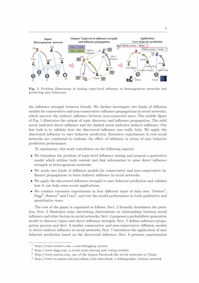
by using the example in Fig. 1. The input (left figure) is a heterogeneous network
consisting of web documents, users, and links between them. To leverage both content
information of web documents and social network structure, we propose a probabilistic
generative model to jointly learn topics and to associate a topic distribution with each
user which indicates his/her interests. Based on the modeling results, we can estimate
3
Smith
AdaBob
Jerry
Ying
Input:
Heterogeneous network
Output: Topics-level influence strength
and influence propagation
Ada
Bob
Smith
Application:
User behavior prediction
Jerry
d1
d2
d3
d4
d5Ying
Topic 1: Avatar
Topic 2: iphone
0.70.3
indirect
influence
direct
influence
0.40.6
0.40.6
0.60.4
0.20.8
Smith
Ada Bob
YingJerry
iphone Avatar
re-tweet a blogwrite a blog
Will she re-tweet iphone ?
click a blog
write a blog
Will he re-tweet Avatar ?
Ying
AAAAAAAAAAAAAAAAAAAAAAAAAAAAAAAAAAAAAA
ngggggggggggggggggggggg
BBBBBBBBBBBBBBBBBBBBo
Je
yyyyyyyyyyyyyyy
Smity
a
Fig. 1 Problem illustration of mining topic-level influence in heterogeneous networks andpredicting user behaviors.
the influence strength between friends. We further investigate two kinds of diffusion
models for conservative and non-conservative influence propagations in social networks,
which uncover the indirect influence between non-connected users. The middle figure
of Fig. 1 illustrates the output of topic discovery and influence propagation. The solid
arrow indicates direct influence and the dashed arrow indicates indirect influence. Our
last task is to validate how the discovered influence can really help. We apply the
discovered influence to user behavior prediction. Extensive experiments in real social
networks are conducted to evaluate the effect of influence in terms of user behavior
prediction performance.
To summarize, this work contributes on the following aspects:
• We formulate the problem of topic-level influence mining and propose a generative
model which utilizes both content and link information to mine direct influence
strength in heterogeneous networks.
• We study two kinds of diffusion models for conservative and non-conservative in-
fluence propagations to learn indirect influence in social networks.
• We apply the discovered influence strength to user behavior prediction and validate
how it can help some social applications.
• We conduct extensive experiments in four different types of data sets: Twitter1,
Digg2, Renren3 and Cora4, and test the model performance in both qualitative and
quantitative ways.
The rest of the paper is organized as follows: Sect. 2 formally formulates the prob-
lem; Sect. 3 illustrates some interesting observations on relationships between social
influence and other factors in social networks; Sect. 4 proposes a probabilistic generative
model to discover topics and direct influence strength; Sect. 5 defines influence propa-
gation process and Sect. 6 studies conservative and non-conservative diffusion models
to derive indirect influence in social networks; Sect. 7 introduces the application of user
behavior prediction based on the discovered influence; Sect. 8 presents experimental
1 http://www.twitter.com, a microblogging system.2 http://www.digg.com, a social news sharing and voting website.3 http://www.renren.com, one of the largest Facebook-like social networks in China.4 http://www.cs.umass.edu/mccallum/code-data.html, a bibliographic citation network

4
results that validate the effectiveness of our methodology; Sect. 9 discusses related work
and Sect. 10 concludes.
2 Problem Formulation
In this section, we introduce several related concepts and then formulate the problem
of mining topic-level influence in heterogeneous networks.
Definition 1 [Heterogeneous Social Network] Define a network as G = (V,D,E),
where V is a set of user nodes, D is a set of document nodes, and E denotes a set
of edges that includes social relationships connecting users and links connecting users
and documents. For each edge euv = (u, v) ∈ E, if there exists an edge between u and
v, euv = 1; otherwise euv = 0. The edges can be directed or undirected.
Many online social networks are heterogeneous consisting of different types of object
nodes. For example, Twitter is comprised of users and microblogs. Digg consists of
users and website URL addresses. Citation network consists of authors and publication
papers. Here, we use “document” to represent different types of associated content (e.g.,
microblog, website, and paper) to each user. Thus links in heterogeneous networks
would contain friendships between users and authoring relationships between users
and documents (links between documents are not considered in this paper). The links
can be directed or undirected. For example, in Twitter and citation networks, the
links between users are directed from normal users to their followers. In Digg social
network, the links between users are undirected. Furthermore, we assume that influence
can propagate along social links, thus we have the following definition.
Definition 2 [Direct and Indirect Influence] Given two user nodes u, v in a het-
erogeneous network G, we denote δv(u) ∈ {R+ ∪ 0} as the influential strength of user
u on user v. Furthermore, if euv = 1, we call δv(u) the direct influence of user u on v;
if euv = 0, we call δv(u) the indirect influence of user u on v.
Direct influence indicates the influence between two users which are connected
while indirect influence indicates the influence of two users which are not connected.
Please note that influence is asymmetric, i.e., δv(u) 6= δu(v). Based on the influence
between node pairs, we can further define the concept of global influence.
Definition 3 [Global Influence] Given a heterogeneous network, Λ(v) ∈ {R+ ∪ 0}
is defined as the global influence of v, which represents the global influential strength
of user v in the network.
The global influence strength has a close relationship with the (local) direct/indirect
influence. For example, if a user has a strong influence on her/his friends, it is very
likely that she/he has a strong global influence.
Our formulation of topic-level influence mining is quite different from existing works
on social influence analysis. Works [1] and [39] study how to qualitatively measure the
existence of influence. Crandall etc. [7] study the correlation between social similarity
and influence. However, they focus on qualitative identification of influence existence,
but do not provide a quantitative measure of the influential strength. Tang et al. [44]
try to learn the influence probabilities according to the network structure and the

5
similarity between nodes. Works [15,47] further investigate how to learn the influence
probabilities from the history of user actions. However, these methods either do not
consider the influence at the topic-level or ignore the influence propagation. The chal-
lenge of our work is how to jointly learn the topics and the topic-level (direct and
indirect) influence from heterogeneous networks. The learned social influence has a
number of immediate applications such as influence maximization [10,25,36], social
action prediction [20,42].
2.1 Intuitions and Our Approach
To summarize, we have two important intuitions for learning influence from heteroge-
nous social networks: (1) influence between users varies over different topics; and (2)
user behaviors are not only influenced by their friends but also their n-degree friends
(e.g., friends’ friends). Indeed, in real networks users may be interested in different
topics, e.g., in the research network an author may be interested in topics “database”
and “data mining”. The influential strength from one’s coauthors on her/him w.r.t.
the two topics might be very different. Actually, this has been qualitatively verified
in sociology [16,29] and quantitatively studied in [44]. More precisely, we can give the
following descriptions for the intuitions:
1. Each node v is associated with a vector ψv ∈ RT of T -dimensional topic distribution
(∑z ψv(z) = 1), where ψv(z) indicates the interest probability of the node (user)
on topic z.
2. Influence can propagate over social networks, thus the influence δv(u) of user u on
v can be direct (euv = 1) or indirect (euv = 0).
3. The behavior of a user is either influenced by his/her friends who have the same
behavior or generated depending on his/her interests.
The last intuition can be better explained by an example on Digg. A user may dig
a story because his friends have digged this story or simply because he is interested in
this topic.
From the technique perspective, our objective is to design a method to learn user
interests (the associated topic distribution) and to estimate user influence simultane-
ously. In this paper, we propose a topic-level influence modeling framework. First, by
combining both textual information and link information in heterogeneous networks,
we present a probabilistic generative model to learn user interests which are represented
as mixtures of topics and direct influence between users simultaneously. Second, based
on direct influence, we study two types of influence propagation mechanism, which are
conservative and non-conservative influence propagations, to derive indirect influence
between users.
Our definition of influence is different from other social factors (e.g., similarity and
tie strength) on the following aspects:
• According to the above intuitions, our definition of influence is based on the dynamic
process of user behaviors, which is related to both content and network structure in
heterogeneous networks. But similarity is more likely to be defined based on content,
while tie strength measures the kinship between two persons which is likely to be
related to common neighborhood.

6
• We investigate influence propagation in this paper, which is an important property
of social influence and can be used in applications such as influence maximization.
Similarity or tie strength does not have the propagation property. Thus they are
different from social influence.
• The obtained influence strength from our model is directed, which means the social
influence from user A to user B is different from that from B to A. While, both
similarity and tie strength are symmetric measurements.
In Section 8.3, we will compare the performance of user behavior prediction based
on influence with the results based on other social factors.
3 Observations
In order to be fully aware of the effect of social influence, we first conduct a series
of analysis before proposing our approach. We focus on four aspects: (1) influence vs.
activity : how one’s activity impacts his/her influence strength? (2) influence vs. degree
centrality : how one’s influence on his friends correlates with his/her degree centrality?
(3) influence vs. similarity : how influence between friends correlates with their sim-
ilarity? and (4) influence vs. n-degree: will a user influence his n-degree friends and
how?
Influence vs. Activity In online heterogeneous networks, some users are much
more active than some others. Taking Renren for example, some users share many web
documents while some others are very silent. Then a question arise: “Is the influence of
a user related to his/her activity?”. To answer this question, we show some observations
and analysis in Renren data set here.
Suppose I(v, d) denotes the connection between a user v and a document d, i.e.,
if user v shares or re-tweets document d, I(v, d) = 1; otherwise I(v, d) = 0. Then the
influence strength of a user v is simply approximated as Eq. (1).
p1(v) = maxd:I(v,d)=1
∑u∈Nb(v) I(u, d)
|Nb(v)|(1)
Thus if v shares a document and his/her friends also shares this document, we think
that the friends are influenced by v. Thus we use the ratio of v’s friends who have the
same actions to estimate the influence strength of v. The maximal influence strength
w.r.t. document in Eq. (1) is used to approximate a user’s influence strength in order
to overcome the noise problem. On the other hand, the number of documents shared
by a user is utilized to indicate the activity of this user, i.e., Act(v) =∑d I(v, d).
We analyze 5000 users from Renren. Fig. 2(a) shows that the number of users with
the same activity value decreases with the increase of user activity factor Act(v) and
most of users share about 0 to 30 web documents. We calculate the average influence
strength of users who share 1, 5, 10, 15, 20, 25, 40, 60, 80, 100 web documents respec-
tively as shown in Fig. 2(b), which demonstrates that with the increase of user activity,
user influence first increases a lot then decreases a little. The result is interesting and
also intuitive. An active user seems to be more likely to influence his/her friends to act
in the same way.
Influence vs. Degree Centrality Besides the connections between users and doc-
uments, there are also links between users in heterogeneous networks. Some users are

7
20 40 60 80 1000
100
200
300
400
Activity
#Use
r
(a) User number v.s. activity
1 5 10 15 20 25 40 60 80 1000
0.1
0.2
0.3
0.4
Activity
Influ
ence
(b) User influence v.s. activity
Fig. 2 User number and user influence strength changing with user activity
0 50 100 150 2000
100
200
300
400
Degree Centrality
#Use
r
(a) User number v.s. degree
1 5 10 15 20 25 40 60 80 1000
0.1
0.2
0.3
0.4
Degree Centrality
Influ
ence
(b) User influence v.s. degree
Fig. 3 User number and user influence strength changing with degree centrality
popular and have many connections with the others. Degree centrality is a measure
in graph theory to determine the relative importance based on the number of links.
Here we try to examine whether users with a higher degree centrality have a stronger
influence in the social network. Again, we study this problem on the Renren data.
The influence strength of a user is estimated by Eq. (1). Fig. 3(a) shows that the user
number first increases and then decreases with the increase of user degree and most of
users have about 10 friends in this social networks. Fig. 3(b) demonstrates that the user
influence strength is weakening with degree, which is consistent to some sociological
research results, i.e., when a user has more and more friends, his/her attention paid to
each friend will be reduced and his/her friend connection will not be so close as before,
which results in his/her influence strength weakening.
Influence vs. Similarity Does influence correlate with similarity in heterogeneous
networks? When the similarity between two nodes increases, how does their potential
influence strength change? In Renren data set, we analyze the relationship between
influence and similarity among node pairs.
First, each user is represented as a keyword vector based on the document content
he/she has shared. Then their similarity is estimated by the Cosine-distance of these
two keyword vectors. The influence from user v to user u is estimated as the ratio of
actions that u has followed v, i.e.,
Inf(v → u) =
∑d:I(v,d)=1 I(u, d)∑d:I(v,d)=1 I(v, d)
(2)
Then the correlation coefficient between influence and similarity calculated by the
above roughly estimation methods in Renren data set is about 0.24. This result demon-
strates that user influence is positive correlated with similarity, but they are still dif-

8
1 2 3 40
0.2
0.4
0.6
degree
p1−
p2
Twitter network
1 2 3 40
0.2
0.4
0.6
degree
p1−
p2
Digg network
1 2 3 40
0.2
0.4
0.6
degree
p1−
p2
Citation network
Fig. 4 n(1 ≤ n ≤ 4)-degree influence in three networks: Twitter, Digg, and Cora.
1 2 3 40
0.05
0.1
0.15
0.2
0.25
degree
p1−
o2
iPhone
1 2 3 40
0.05
0.1
0.15
0.2
0.25
degree
p1−
p2Obama
1 2 3 40
0.05
0.1
0.15
0.2
0.25
degreep1
−p2
Avatar
Fig. 5 Topic-level influence on three topics: “iPhone”, “Obama”, and “Avatar”.
ferent factors with different effects in social networks as their correlation coefficient is
not so big.
Influence vs. n-degree Influence propagates over social networks as discussed in
Sect. 2. In order to verify the existence of indirect influence and to study the influence
propagation mechanism, we conduct an analysis on the influence strength changing
with propagation length.
We estimate the influence strength after i-step propagation as Eq. (3)
p1(v) = maxd:I(v,d)=1
∑u∈Nbi(v)
I(u, d)
|Nbi(v)|(3)
To test the effect of influence propagation, Eq. (3) extends Eq. (1) by enlarging v’s
neighborhood to Nbi(v). Nbi(v) includes v’s possible accessed friends after i-step prop-
agation. For example, when influence propagates one step, Nb1(v) includes v’s friends’
friends (named as two-degree friends in [13,46]) which can be accessed through one of
v’s friends who has shared d, i.e., if w ∈ Nb(v) and I(w, d) = 1 and u ∈ Nb(w), then
u ∈ Nb1(v).
In order to form a close community, the 5000 users in Renren data set are selected
from a user’s two-degree friend neighborhood. Thus we calculate each user’s influence
strength on one-degree friends as well as that on two-degree friends, which are 0.2
and 0.05 respectively. Thus the two-degree influence strength decreases a lot, which
is only 25% of one-degree influence strength in Renren data set. Besides, to further
study influence strength changing with propagation step, we calculate three and four-
degree influence strength in other three heterogeneous networks – Twitter, Digg, and
Cora. Fig. 4 demonstrates that indirect influence also exists in other social networks.
For example, on Renren, when a user shares an interesting poster, his/her friends’
friends (2-degree friends) averagely have a 20+% higher probability to follow him/her.
However, the influence strength decreases with the increase of propagation length on

9
λx
x
x
x
w
z
sy
w
z
γ
w
zw
z
A
Influencing Users Influenced Users
u4
u3
u2
ut
u1
Heterogeneous Network
Influencing user
ut
u1Inflff uen
document
write
d1
d2
d2
θ
f
y
Fig. 6 Probabilistic generative model to estimate direct influence strength
average. Furthermore, the influence patterns on these networks are quite different. For
example, influence on Twitter is small and gradually decreases with the increase of
degree. While on Digg, influence tapers off quickly with the increase of propagation
length. Furthermore, we analyze the topic-level influence on Twitter as shown in Fig. 5.
We study the n-degree influence on three topics: “Obama”, “iphone” and “Avatar”.
These influence changing patterns are different. An interesting phenomenon is that on
some topics the two-degree influence is even stronger than the one-degree influence
(e.g., on “Avatar”). his is because “Avatar” is a very popular topic, on which the users
may be mainly influenced by the global trend (via conformity [24]).
In summary, according to the approximate analysis above, we have the following
observations:
• Active users are likely to be more influential. But when the user activity increases
to a certain level, it may be no longer the major factor to impact the user influence.
• When a user has more friends, his/her attention paid to each friend would be
reduced and his/her friend connection would not be so close as before, which may
result in his/her influence strength weakening.
• User influence is positive correlated with similarity, but they are still different fac-
tors with different effects in social networks.
• Indirect influence exists in social networks, which decreases with the increase of
propagation length generally. And influence strength changing patterns vary with
topics.
4 Mining Influence in Heterogeneous Networks
Influence is interacted with many potential factors, e.g., similarity and correlation [1,
7]. Here we have two general assumptions in order to model the influence strength
quantitatively.
Assumption 1 Users with similar interests have a stronger influence on each other.
This assumption actually corresponds to the influence and selection theory [1].
We have observed that user influence is positive correlated with similarity in Sect 3.
In real networks, the similarity can be calculated based on the content information
associated with each user. Thus, influence can be represented as to which extent the

10
Table 1 Variable descriptions
Notation Descriptionx, x′ the influenced/influencing userw,w′ words in the associated documentz, z′ topic assignment to each wordd, d′ document associated with influenced/influencing userAx the user list who may influence xy the influencing user from Axs the label denoting either influencing or notW the number of words in the data setT the number of topics to be extractedθ the topic mixture of influencing usersψ innovative topic mixture of usersφ word distribution for each topicγ the influence mixture of usersλ the parameter to draw the label sα the Dirichlet prior for hidden variables
textual content is “copied” from the influencing nodes. For example, in the citation
network, if the content of document d1 is very similar to that of document d2, we may
deem that d1 “copies” a lot of ideas from d2, thus d1 is influenced by d2 a lot.
Assumption 2 Users whose actions frequently correlate have a stronger influence on
each other.
The co-occurrence frequency is often used to indicate the correlation strength be-
tween two nodes, which is denoted by the weights of edges in networks. Thus the influ-
ence strength between two nodes would be enlarged by their frequent co-occurrence.
For example, if author a cites a number of papers of author b, then a should be strongly
influenced by b. For another example on Twitter, if user a replies or re-tweets many
microblogs posted by user b, then it is very likely that b has a strong influence on a.
Based on these considerations, we propose a probabilistic generative model to
jointly learn user interests and direct influence strength between users quantitatively.
4.1 Probabilistic Generative Model
In Sect. 3 we have observed that influence strength varies with topics. Thus in this
section we design a model to mine topics and influence strength simultaneously. The
model combines the content information and network structure in heterogeneous net-
works as shown in Fig. 6. Based on the intuitions in Sect 2, we assume that the behavior
of each influenced user can be generated in two ways, either depending on his/her own
interests or influenced by one of his/her friends. E.g., when a user shares a blog on Ren-
ren, he/she may like its content or follow the action of one of his/her friends who also
share it. Thus the proposed model consists of the following two parts, and the whole
generative process are illustrated in Alg. 1 (Table 1 lists the descriptions of variables).
• User interest modeling As shown in the middle part of Fig. 6, each user x
is represented as a multinomial distribution over topics ψ, which indicates user
interests. We assume that topics of documents are generated based on user interests.
Then each word w in documents is generated from one topic z selected from the

11
foreach influencing user x′ doforeach associated document d′ do
foreach word i ∈ d′ doDraw a topic z′
d′,i∼ multi(ψx) from the topic mixture of user x′
d′,i;
Draw a word w′
d′,i∼ multi(φzd,i ) from z′
d′,i-specific word distribution;
end
end
end
foreach influenced user x do
foreach associated documents d do
foreach word i ∈ d doToss a coin sd,i ∼ bernoulli(λxd,i), where
λxd,i = p(s = 0|xd,i) ∼ beta(αλs0 , αλs1 ) which indicates the proportion
between the innovation and influenced probability of xd,i;if sd,i = 0 then
Draw a influencing user yd,i ∼ multi(γx) from the user list Ax;Draw a topic zd,i ∼ multi(θy) from the topic mixture of yd,i;
end
if sd,i = 1 thenDraw a topic zd,i ∼ multi(ψx) from the topic mixture of xd,i;
end
Draw a word wd,i ∼ multi(φzd,i ) from zd,i-specific word distribution;
end
end
end
Algorithm 1: Probabilistic generative process
distribution. The details of the generative process are illustrated in the first iteration
of Alg. 1.
• Influence strength mining The right part of Fig. 6 illustrates influence strength
modeling. The parameter s, which is generated from a Bernoulli distribution with
parameter λ, is used to control the influence situation. We assume that when s = 1,
the behavior is generated based on his/her own interests, while when s = 0, the
behavior of the user is influenced by one of his/her friends. Then another parameter
γ is used to indicate the influence strength from candidate user set Ax to user x,
based on which one influencing user y is selected from Ax. At last, a topic is
generated from the mixture of topics of a user – the user himself/herself x or one of
his/her friends y, based on which the word w is generated. This part corresponds
to the second iteration of Alg. 1.
In the above generative process, Ax is the candidate influencing user set w.r.t. x,
thus Ax changes with x. Besides, Ax is determined by real applications, which considers
both directed and undirected links between users. For example, in Twitter network Axdenotes the users whom a blog is re-tweeted from while in citation networks it denotes
the authors of cited papers. In these networks, the links between users are directed.
In some other networks, such as Renren and Digg, Ax denotes the friends of user x
who also share or dig the same story, and the links are undirected. Thus the proposed
model is able to handle both types of cases.

12
4.2 Model Learning via Gibbs Sampling
We employ Gibbs sampling to estimate the model. Gibbs sampling is an algorithm
to approximate the joint distribution of multiple variables by drawing a sequence of
samples, which iteratively updates each latent variable under the condition of fixing
remaining variables. We list the update equations for each variable as below and the
details of derivation can refer to the appendix. In all the update equations, N(∗) is
the function which stores the number of samples during Gibbs sampling. For example,
Nx,z,s(x, z, 1) represents the number of samples of topics z which are supposed to be
generated from user x when s = 1.
p(si = 0|s−i, xi, zi, .) ∝
Nx′,z′ (yi,zi)+Ny,z,s(yi,zi,0)+αθNx′ (yi)+Ny,s(yi,0)+T ·αθ
·Nx,s(xi,0)+αλs0
Nx(xi)+αλs0+αλs1
(4)
p(si = 1|s−i, xi, zi, .) ∝
Nx,z,s(xi,zi,1)+αψNx,s(xi,1)+T ·αψ
·Nx,s(xi,1)+αλs1
Nx(xi)+αλs0+αλs1
(5)
p(yi|y−i, si = 0, di, xi, zi, Ax, .) ∝
Nx,y,s(xi,yi,0)+αγNx,s(xi,0)+|Ax|·αγ
·Nx′,z′ (yi,zi)+Ny,z,s(yi,zi,0)+αθ
Nx′ (yi)+Ny,s(yi,0)+T ·αθ(6)
p(zi|z−i, si = 0, wi, .) ∝
Nx′,z′ (yi,zi)+Ny,z,s(yi,zi,0)+αθNx′ (yi)+Ny,s(yi,0)+T ·αθ
·Nw,z(wi,zi)+Nw′,z′ (w
′
i,z′
i)+αφNz(zi)+Nz′ (zi)+W ·αφ
(7)
p(zi|z−i, si = 1, wi, .) ∝
Nx,z,s(xi,zi,1)+αψNx,s(xi,1)+T ·αψ
·Nw,z(wi,zi)+Nw′,z′ (w
′
i,z′
i)+αφNz(zi)+Nz′ (zi)+W ·αφ
(8)
Through the Gibbs sampling process, we obtain the sampled coin si, influencing
user yi, and topic zi for each word. Then the influence strength can be estimated by
Eq.(9), which are averaged over the sampling chain after convergence. K denotes the
length of the sampling chain.
δx(y) = γx(y) =1
K
K∑
i=1
Nx,y,s(x, y, 0)i + αγ
Nx,s(x, 0)i + |A| · αγ(9)
The equation is consistent to our assumptions in a statistical way. Take citation
networks for example. If author x cites more papers of author y and “copies” more
content from y, Nx,y,s(x, y, 0) will be larger, and thus the influence from y to x will
be stronger. Besides, it is easy to get that∑|Ax|y=1 δx(y) = 1, i.e., the sum of influence
on user x from all the users obtained in the model equals to 1. And the model does
not consider the influence between the nodes which are not connected, i.e., δx(y) = 0
when x and y are not connected.
Furthermore, we can estimate the topic-level influence strength. Suppose δx,z(y)
represents the influence strength from user y to user x on the topic z, which satisfy that
δx(y) =∑Tz=1 δx,z(y). Thus the topic-level influence can be estimated by Eq. (10).
δx,z(y) =1
K
K∑
i=1
Nx,y,z,s(x, y, z, 0)i + 1
T · αγ
Nx,s(x, 0)i + |A| · αγ(10)

13
a1 a2 a3
a3
a1
a2
a4
(a) (b)
Fig. 7 Influence propagation
5 Influence Propagation and Aggregation
The above probabilistic model only discovers direct influence, but does not consider
indirect influence. In reality, like information or virus, influence also propagates over
networks, which produces different types of indirect influence. Take Fig. 7(a) for ex-
ample. If a1 influences a2 and a2 influences a3, then a1 will influence a3 potentially,
i.e., two-degree of influence. Fig. 7(b) demonstrates the influence enhancement: if a1
influences a3 and a4 while a3 and a4 also have an influence on a2, then the influence
from a1 to a2 should be enhanced. The observations in Sect 3 have demonstrated the
existence of indirect influence. Based on these observations, we study atomic and it-
erative influence propagation process over social networks in this section, via which
indirect influence can be obtained from direct influence and global influence strength
can be estimated.
5.1 Atomic Influence Propagation
As shown in Fig. 7, we observe there are two basic processes for influence propagation.
• Concatenation The indirect influence from a1 to a3 in Fig. 7(a) can be modeled
as a concatenate result of the direct influence from a1 to a2 and the direct influence
from a2 to a3.
• Aggregation The enhancement of the influence from a1 to a2 in Fig. 7(b) can be
defined as an aggregate result of the direct influence among the neighborhood of
a1 and a2.
Therefore, the atomic influence propagation is defined as:
δv(u) = ♦(∀w ∈ Nb(v) : δv(w) ◦ δw(u)) (11)
where Nb(v) is the set of neighbors of node v. ◦ is the concatenation function and ♦
is the aggregation function.
In real processes, multiplication operation or minimum value is often used as con-
catenation function while addition operation or maximum value is used as the aggre-
gation function. In particular, if we employ multiplication and addition operations to
replace the concatenation and aggregation function in Eq. (11) respectively, then the
atomic influence propagation can be instantiated as:
δv(u) =∑
w∈Nb(v)
δv(w) · δw(u) (12)
Suppose ∆v represents the vector of the influence strength from all the nodes in
the network on node v, i.e., ∆v = (δv(u1), δv(u2), ..., δv(un)). And we use superscript

14
to denote the propagation step, i.e., ∆0 denotes the initial influence strength and ∆1
denotes the influence strength after the atomic propagation. Then the atomic influence
propagation can be represented as the matrix multiplication.
∆1v = ∆
0v ·M (13)
where M is the transition matrix and M = (∆v1 ;∆v2 ; ...;∆vn), i.e., each element in
the transition matrix M(v, u) = δv(u).
5.2 Iterative Influence Propagation
In reality, the indirect influence along longer paths, e.g., three-degree or four-degree
influence, also have effect on the nodes in a network. In another word, influence can
propagate iteratively to collect the contribute of influence on longer paths. Thus the
atomic influence propagation should be performed iteratively to propagate direct in-
fluence over the entire network. Thus the influence strength on k-length paths can be
calculated by k steps of atomic propagations.
If the atomic propagation is defined as Eq. (13), the influence strength vector after
k-step atomic propagation can be calculated by the matrix powering operation.
∆kv = ∆
k−1v ·M = ∆
0v ·M
k (14)
where Mk =Mk−1 ·M . ∆k denotes the influence strength vector on k-length paths.
Formally, we define the iterative influence propagation as following:
• Enumerate all paths between each two nodes.
• Calculate the influence propagation strength on each path via a concatenation
function.
• Combine the influence strength on all the paths via an aggregation function.
Suppose the final influence strength between two nodes after k-step iterative prop-
agation is denoted as ∆fk . Based on the above definition, it should collect all the
contributes of the influence strength on paths with the length ranging from 0 to k, i.e.,
∆fk = ♦(∀i ∈ {0, 1, 2, ..., k} : ∆i) (15)
If addition operation is used as the aggregation function, ∆fk can be inferred from
the sequences of propagation via a weighted linear combination [18]:
∆fk =
k∑
i=0
βi∆i (16)
βi denotes the weight for the influence strength on i-length paths, i.e., ∆i.
Intuitively, the effect of the influence on shorter paths should be larger than the
one on longer paths as the iterative propagation process brings in more outside infor-
mation. In Sect 3 we have also found that indirect strength decreases with the increase
of propagation length generally. Therefore, βi should decrease with the increase of it-
eration step i. Different strategies can be employed to assign the weights. In the next
section, we will study two kinds of strategies, which are conservative propagation and
non-conservative propagation respectively.

15
5.3 Global Influence Estimation
Global influence is to measure one’s influential ability over the whole network. For
example, some authors are very influential on the topic of “data mining”. In this
section, we propose one way to estimate one node’s global influence over the whole
network.
Intuitively, the global influence of one node Λ(u) should be related to its influence
on all the other nodes in the network. If one node strongly influences many other nodes,
its global influence might be also strong. Therefore the global influence of a node is
defined as an aggregation of its influence on the other nodes, specifically,
Λ(u) =∑
v
δv(u) (17)
The influence scores δv(u) include both direct and indirect influences.
6 Conservative and Non-conservative Propagation
In this section, we describe two types of diffusion process - conservative and non-
conservative diffusion process, based on which we propose two kinds of methods to
propagate influence over the network and to obtain indirect influence strength.
First, we formally define a propagation process over a network.
Definition 4 [Propagation Process] A propagation process over a network G is
defined as a function {Ft(w) : (R+ ∪ {0})|V | → (R+ ∪ {0})|V |}, where V is the set of
nodes in G. w is a V -dimensional vector, which represents a weight distribution over
the nodes in the network. t denotes propagation step.
Therefore, in a propagation process, each node in a network is first initialized with
some mass, which is denoted as the weight of the node. Then via each step of prop-
agation, some nodes transfer a part of the weights to their neighbors. Thus through
a t-step propagation process, a |V |-dimensional non-negative vector is mapped to an-
other |V |-dimensional non-negative vector. In particular, when t = 1, the propagation
is atomic propagation.
6.1 Conservative Propagation
Definition 5 [Conservative Propagation] For a propagation process F , if ∀w ∈
(R+ ∪ {0})|V |,||w||1 = ||F (w)||1,i.e., it preserves the sum of the entries, we call the
propagation process conservative propagation.
Therefore, conservative propagation simply redistributes the weights among the
nodes in the network and keeps the sum of weights constant. There are many con-
servative propagation examples in the real world. Take the circulation of money for
example. At each step of propagation, some nodes transfer a fraction of their money
to their neighbors. But the total money in the network does not change. Traffic trans-
portation and energy cycle are also conservative propagations as the total traffic or
energy does not change with the propagation process.

16
Mathematically, random walk is a canonical example of conservative propagation.
In a random walk, a particle starts to locate on a node. Then at each step, the particle
selects one of the out-neighbors at random and moves to that node. A weight vector
is used to represent the probability with which the particle can be found on each
node. Thus the sum of the weights equals to one. And after iterative propagations, the
probabilities of finding the particle on the nodes change, but the sum remains to be
one all the time.
PageRank is a classical random walk model, which is represented as:
pr(w) = (1− β) · w0 + β · pr(w) ·M (18)
M is a transition matrix, in which the element M(a, b) denotes the transfer proba-
bility from node a to b. β is a damping factor which is used to ensure the stationary
probability distribution of the propagation. 1−β is the restart probability, which gives
the probability distribution when the random walk transition restarts. w0 is the initial
weight distribution, which is usually set to be uniform vector. Personalized PageRank
[22] extends the model by setting w0 to be a non-uniform starting vector.
6.1.1 Conservative Influence Propagation
We model the conservative influence propagation as a personalized PageRank in a
network as Eq. (19).
∆ft = (1− β) ·∆0 + β ·∆ft−1 ·M (19)
The propagation probability matrix M can be set in various ways. If we use direct
influence strength to define the propagation probability, i.e., M(v, u) = δ0v(u), then∑uM(v, u) = 1. It is easy to prove that the sum of influence strength from all the
nodes on one node v remains to be one after influence propagation, i.e., ||∆ftv ||1 = 1.
Thus Eq. (19) defines a conservative influence propagation.
This conservative influence propagation provides a strategy for the combination
process in the iterative propagation. From Eq. (19), it is easy to get that
∆ft = (1− β) ·∆0 ·
t−1∑
i=0
(βi ·M i) +∆0 · βt ·M t (20)
As the influence vector on t-length path is ∆t = ∆0 ·M t,
∆ft = (1− β) ·
t−1∑
i=0
(βi ·∆i) + βt ·∆t (21)
Thus the conservative influence propagation defined in Eq. (19) assigns different weights
to the influences on different-length paths.
β is a damping factor, i.e., 0 ≤ β ≤ 1. Thus when t increases, βt decreases, which
makes the effect of influence on longer paths smaller.

17
6.2 Non-conservative Propagation
Definition 6 [Non-conservative Propagation] For a propagation process F , if
∃w ∈ (R+∪{0})|V |,||w||1 6= ||F (w)||1, we call the propagation process non-conservative
propagation.
Compared with conservative propagation, non-conservative propagation does not
keep the sum of weights constant. There are also many non-conservative propagation
examples in the real world. Take the spread of a virus for example. Suppose a virus is
propagating over the social network. When one infected node infects its neighbors, it is
still infected. Thus the total number of infected nodes is increased with time. Therefore,
the spread of virus is a kind of non-conservative process. Besides, information diffusion
and oral advertising are also non-conservative propagations as the number of nodes
which accept the information or advertisement increases with propagation step.
Alpha-Centrality, which was introduced by Bonacich [3,4], can be used to model
non-conservative propagation. The Alpha-Centrality vector c(w) is defined as the so-
lution of the following equation:
ct(w) = w0 + β · ct−1(w) ·M (22)
β is a damping factor. The starting vector w0 is usually set to be in-degree centrality.
And M uses the adjacency matrix.
When β < 1|λ1|
(where λ1 is the largest eigenvalue of M), we can get that c(w) =
w0 · (I − βM)−1, where I is the identity matrix of size n. Using the identity
∞∑
t=1
(βt ·M t) = (I − β ·M)−1 − I (23)
we can get
c(w) = w0 · (I − β ·M)−1 = w0 ·∞∑
t=0
(βt ·M t) (24)
Besides Alpha-Centrality, Katz score [23], SenderRank [27] and eigenvector cen-
trality [2] are other examples of non-conservative mathematical metrics.
6.2.1 Non-conservative Influence Propagation
We model the non-conservative influence propagation process in the form of Alpha-
Centrality as Eq. (25).
∆ft = ∆
0 + β ·∆ft−1 ·M (25)
For Alpha-Centrality, M is usually set to be adjacency matrix. Here we also use direct
influence strength to define the transition matrix M , i.e., M(v, u) = δv(u). It is easy
to prove that the sum of influence strength from all the nodes on node v increases
with non-conservative propagation step, i.e., ||∆ftv ||1 > 1 . Thus Eq. (25) defines a
non-conservative propagation for local influence.
This non-conservative influence propagation provides another strategy for the com-
bination process in the iterative propagation. From Eq. (25), we can get

18
∆ft = ∆
0 ·t∑
i=0
(βi ·M i) =t∑
i=0
βi ·∆i (26)
Thus it assigns different weights to the influence strength on different-length paths.
However, the weight assignment strategy is different from conservative propagation
referring to Eq. (21).
6.3 Comparison and Explanation
Both conservative and non-conservative influence propagations collect all the con-
tributes of direct and indirect influence on the propagating paths. And both of them
define a weight assignment strategy to distinguish the effect of influence on different-
length paths. The major difference between these two types of models is that conser-
vative propagation keeps the sum of influence in the whole network constant while
non-conservative propagation does not.
Intuitively, indirect influence strength on shorter-paths should be more reliable
since there have been fewer propagation steps. The more iteration steps, the more
outside information will be brought. Thus, both conservative and non-conservative
propagations utilize a damping factor β to penalize larger t-step propagations. As
0 ≤ β ≤ 1, when t increases, βt decreases greatly, which makes the effect of influence
on (t+1)-length paths very small. In another word, we do not need to iterate influence
propagation for many times to obtain the final indirect influence, i.e., t can be set
as a small number. Besides, when β = 0, both conservative and non-conservative
propagations only utilize direct influence and ignore the effect of indirect influence.
7 User Behavior Prediction
The learned influence strength can be used to help with many applications. Here we
illustrate one application on user behavior prediction, i.e., how the learned influence
can help improve the performance of user behavior prediction.
We evaluate our approach for user behavior prediction on Renren, Twitter and
Digg. The user behavior is defined as one time connection between a user and a doc-
ument. We here take Digg as the example for explanation. Intuitively, if more friends
of a user dig a story, there is a larger probability that the user will also dig it. Thus a
vote-based relational neighbor classifier [33] can be used as a baseline. Then, we use the
influence strength obtained from our approach to distinguish different friends’ weights
and estimate the probability of users’ digging stories as follows:
p(d|u) =1∑
v δu(v)
∑
v∈Nb(u)
δu(v)p(d|v) (27)
where Nb(u) denotes the friends of u.
Besides, the similarity between users can also be used to distinguish different
friends’ weights in the above intuitive method for prediction. Thus the prediction proba-
bility is estimated as Eq.(28) for comparison, where the similarity between users s(v, u)
is calculated as the Euclidean distance of user distributions over topics.

19
p(d|u) =1∑
v s(v, u)
∑
v∈Nb(u)
s(v, u)p(d|v) (28)
We will test the user behavior prediction performance based on the above three
methods in the following experiments and demonstrate the effect of influence strength
obtained from both conservative and non-conservative influence propagations for social
network applications.
8 Experiments
In this section, we present various experiments to evaluate the efficiency and effective-
ness of the proposed approach. The data sets and codes are publicly available5.
8.1 Experimental Setup
Data Sets We prepare four different types of heterogeneous networks for our ex-
periments, including Renren, Twitter, Digg and citation networks. Renren is a very
popular FaceBook-style social website in China, on which users (especially the under-
graduate and graduate students) connect with their classmates or friends and share
interesting web content. Twitter is a microblog website, on which users can publish
blogs and re-tweet friends’ blogs. Digg is a different type of social website, on which
users can submit, dig and comment on stories. Users also have links to their friends,
which indicate their relationship. We collect user relationship and document content
from these websites.
• Renren social network The data contains 5000 users and the web content shared
by these users in one month which includes about 10000 documents and 30000
words.
• Twitter social network The dataset includes about millions of microblogs re-
lated to about 40000 users and 50000 keywords (removing the stop words and the
infrequent words).
• Digg social network The data contains about 1 million stories related to 10000
users and 30000 keywords, in which we aim to mine user influence as well.
• Citation network We crawled the citation data of about 1000 documents from
the Internet on several specific topics, e.g., “topic models”, “sentiment analysis”,
“association rule mining”, “privacy security” and etc. Besides, the public citation
data set Cora is also used in our experiments.
We apply our model to the above four data sets. The algorithms are implemented
in C++ and run on an Intel Core 2 T7200 and a processor with 2GB DDR2 RAM.
The parameters of the model will be discussed in the following subsections.
Evaluation Aspects We evaluate our method on the following three aspects:
Influence strength prediction As it is more intuitive and easier for people to
distinguish the influence strength in citation networks, we manually label the citation
data and then test the influence prediction performance in it. We compare the results
5 http://arnetminer.org/heterinf

20
0.5
0.6
0.7
0.8
10 15 20 30 50
#topic
AUC
Data1_M1 Data1_M2 Data2_M1 Data2_M2
Fig. 8 Influence prediction performance comparison
of our approach with previous work [9] to demonstrate our model’s better performance
in terms of influence prediction.
User behavior prediction We use the derived influence strength to help predict
user behaviors and compare the prediction performance with that of baseline as well
as the method based on user similarity as described in Sect. 7. The results demon-
strate how the quantitative measurement of the influence can benefit social network
applications.
Topic-level influence case study We show several case studies to demonstrate
concrete influence weights between users and show how effectively our method can
identify topic-level influence. In particular, we study the global influence of authors in
citation networks to demonstrate semantic meaning of topic-level influence. And we
compare the results with that of previous work [44] which can also be used to mine
topic-level influence to demonstrate the better performance of our approach.
8.2 Influence Prediction
In work [9], researchers evaluated the document influence prediction performance in a
manually labeled data set. We use the same data from the authors and also test the
influence prediction performance of our model in it. However, the data set, which only
contains 22 citing documents and 132 documents in all, is so small that the results
could be ad-hoc sometimes. Therefore, besides using this data, we also manually label
document influence strength in a larger data set with about 1000 documents. We
classify the influence strength into three levels: 1, 2, 3. Similar to [9], we use the
quality measure, averaged AUC (Area Under the ROC Curve) values for the decision
boundaries “1 vs. 2, 3” and “1, 2 vs. 3” for each citing document, to evaluate the
prediction performance.
Fig. 8 shows the comparative results in these two data sets, where Data1 is the
small data set obtained from authors of [9] while Data2 is our larger labeled data set.
M1 and M2 are used to denote our model and the model in [9] respectively. And we
use the real and dash lines to distinguish the results of these two models in the figure.
We calculate all the AUC values with the number of topics changing from 10 to 50.
Thus this figure demonstrates that in the small data set our model can achieve as good
prediction performance as the work in [9] while in the larger data set, our prediction
performance is better than theirs.
Furthermore, we compare the influence prediction performance before and after
influence propagation in our labeled data set. The results prove that the influence pre-

21
Table 2 Conservative and non-conservative influence propagation effect on user behaviorprediction
PPP
PP
pmethod
baseline DIinfluence propagation
stepsβ = 0.3 β = 0.5 β = 0.8
CIP NCIP CIP NCIP CIP NCIP
Avg0.101 0.160
t = 1 0.168 0.168 0.168 0.168 0.172 0.168t = 5 0.168 0.168 0.170 0.170 0.180 0.175t = 10 0.168 0.168 0.170 0.170 0.180 0.178
Var0.011 0.048
t = 1 0.044 0.045 0.041 0.044 0.039 0.042t = 5 0.044 0.045 0.042 0.043 0.041 0.041t = 10 0.044 0.045 0.043 0.042 0.041 0.041
0.1 0.2 0.3 0.4 0.5 0.6 0.7 0.8 0.90
0.1
0.2
0.3
0.4
0.5
0.6
threshold
Pre
cisi
on
baselineno propagationconservative propagationnon−conservative propagation
Fig. 9 User behavior prediction precision on Renren network
diction performance is enhanced after influence propagation (AUC values are enhanced
from 0.69 to o.76). Moreover, the influence prediction performance is robust to the pa-
rameters t and β. In particular, when t changes, the performance changes little, which
is consistent to the observation in Fig. 4. It means that influence does propagate over
the network, but the effect of propagation is reduced with propagation step.
8.3 User Behavior Prediction
We employ our model to discover the concrete influence strength between the 5000
users in Renren social networks. Then we apply the learned influence strength to user
behavior prediction as described in Sect. 7. In particular, the parameters which are the
damping factor β and iteration step t for both conservative and non-conservative influ-
ence propagations are varied to test the effect of influence propagation process. About
36000 tuples in Renren data set are used as testing samples. Each tuple represents that
a user shares a web document, whose probability is estimated as Eq. (27).
The average and variance values of the predicted probabilities for all the samples
are calculated and shown in Table 2, where DI denotes direct influence, CIP and
NCIP denote conservative and non-conservative influence propagations respectively.
The results demonstrate that using influence, especially the propagated influence, can
greatly improve the predicted probabilities. But the parameters t and β as well as the
propagation mechanism do not affect the probabilities a lot.
Then given a threshold, we calculate the prediction precision, which means how
many testing samples’ probabilities are larger than the threshold. Fig. 9 shows four
curves of prediction precision changing with the threshold in Renren data set, which in-
dicate the performance of baseline, using direct influence without influence propagation,
conservative and non-conservative influence propagations with parameter β = 0.8, t = 5
respectively. The results demonstrate that influence-based behavior prediction ap-
proach outperforms the baseline. Thus it proves that the influence obtained from our

22
Table 3 Behavior prediction probability
Digg Social NetworkXX
XX
XXX
pmethod
baseline similarity DI NCIF
average 0.112 0.121 0.366 0.405variance 0.006 0.008 0.075 0.048
Twitter Social NetworkXX
XX
XXX
pmethod
baseline similarity DI NCIF
average 0.215 0.222 0.319 0.310variance 0.078 0.089 0.129 0.136
0.1 0.2 0.3 0.4 0.5 0.6 0.7 0.8 0.90
0.1
0.2
0.3
0.4
0.5
0.6
0.7
0.8
0.9
threshold
Pre
cisi
on
indirect influencesimilaritybaselinedirect influence
Fig. 10 User behavior prediction precision on Digg network
0.1 0.2 0.3 0.4 0.5 0.6 0.7 0.8 0.90
0.1
0.2
0.3
0.4
0.5
0.6
0.7
threshold
Pre
cisi
on
indirect influencesimilaritybaselinedirect influence
Fig. 11 User behavior prediction precision on Twitter network
model benefits the user behavior prediction greatly. Moreover both conservative and
non-conservative influence propagations improve the prediction precision and almost
achieve the same performance.
Besides, we apply our model to the application of user behavior predication in Twit-
ter and Digg social networks. In this experiment, we employ non-conservative influence
propagation with t = 5, β = 0.8 to obtain indirect influence. We randomly select about
3000 tuples from Digg and Twitter data sets as testing samples and estimate their
probabilities. Table 3 shows the average and variance values of the predicted proba-
bilities for all the samples. The prediction precision curves for these two data sets are
shown in Fig. 10 and 11 respectively. The results demonstrate that influence-based be-
havior prediction approach outperforms the baseline and the similarity-based method.
In particular, it shows that influence propagation process enhances the user behav-
ior prediction performance in Digg social network but it takes little effect in Twitter
social network. Furthermore, comparing these two figures, we can get that the effect
of influence in Digg social network is larger than that in Twitter social network. The
conclusion is consistent to the observation in Fig. 4.
23
topics over time: a
non-markov
continuous-time
model of topical
trends
probabilistic latent
semantic indexing
gap: a factor model
for discrete data
latent dirichlet
allocation
A McCallum & X
Wang
a variational
principle for
graphical models
topic and role
discovery in social
networks
T HofmannM JordanH Attias
expectation-
propagation for the
generative aspect
model M Rosen-Zvi & T
Griffiths
probabilistic author
topic models
information
discovery
correlated topic
models
J Lafferty
dynamic topic
models
a variational
bayesian
framework for
graphical models
the author-recipient-
topic model for topic
and role discovery in
social networks
D Blei
the author-topic
model for authors
and documents
Fig. 12 Document influence case study
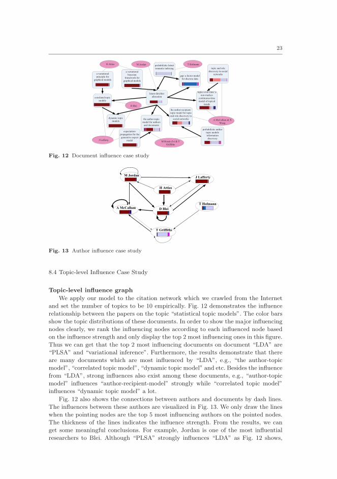
Fig. 13 Author influence case study
8.4 Topic-level Influence Case Study
Topic-level influence graph
We apply our model to the citation network which we crawled from the Internet
and set the number of topics to be 10 empirically. Fig. 12 demonstrates the influence
relationship between the papers on the topic “statistical topic models”. The color bars
show the topic distributions of these documents. In order to show the major influencing
nodes clearly, we rank the influencing nodes according to each influenced node based
on the influence strength and only display the top 2 most influencing ones in this figure.
Thus we can get that the top 2 most influencing documents on document “LDA” are
“PLSA” and “variational inference”. Furthermore, the results demonstrate that there
are many documents which are most influenced by “LDA”, e.g., “the author-topic
model”, “correlated topic model”, “dynamic topic model” and etc. Besides the influence
from “LDA”, strong influences also exist among these documents, e.g., “author-topic
model” influences “author-recipient-model” strongly while “correlated topic model”
influences “dynamic topic model” a lot.
Fig. 12 also shows the connections between authors and documents by dash lines.
The influences between these authors are visualized in Fig. 13. We only draw the lines
when the pointing nodes are the top 5 most influencing authors on the pointed nodes.
The thickness of the lines indicates the influence strength. From the results, we can
get some meaningful conclusions. For example, Jordan is one of the most influential
researchers to Blei. Although “PLSA” strongly influences “LDA” as Fig. 12 shows,

24
Table 4 Author ranking on “statistical topic models”
Direct InfluenceIndirect Influence
Pagerankt = 1 t = 5
TM Cover D Blei D Blei M JordanA McCallum A McCallum A McCallum D BleiD Blei TM Cover M Jordan J LaffertyM Jordan M Jordan TM Cover A McCallumP Kantor P Kantor P Kantor Z Ghahramani
Table 5 Influence aggregation values on topics
Topic OODB IR DM DBPMaximal value 2.525 2.333 3.877 3.607Minimal value 0.0005 0.001 0.0006 0.0009Average value 0.078 0.091 0.095 0.087D DeWitt 1.487 0.181 1.087 3.607
M Stonebraker 2.525 0.632 0.481 2.851
C Faloutsos 0.357 0.242 1.571 1.187
W Bruce 0.538 2.333 0.172 0.483R Agrawal 0.518 0.189 3.877 0.600J Han 0.666 0.138 2.029 0.240
Hofmann does not have a great influence on Blei. The reason is that the area of Hof-
mann varies from the area of Blei (this can be observed from the topic distributions
represented by colored bars) and furthermore Blei only cited few documents of Hof-
mann, i.e., correlation value is small. Other interesting results are also obtained, e.g.,
the influence of Blei on Lafferty is larger than the influence of Lafferty on Blei. Be-
sides, the self-loop lines which indicate the self-influence show Jordan and Blei influence
themselves greatly.
Topic-level global influence illustration
Table 4 shows an example of author ranking by estimated global influence on “sta-
tistical topic models” (t denotes the number of propagation steps). The results are very
meaningful. If one node has a high reputation over the whole network, it can be treated
as a key node which is very influential over the whole network. In another word, au-
thority of one node can also be used to represent its global influence from some point of
view. Therefore, we can employ PageRank [35,19] over topic-level networks to estimate
the nodes’ global influence on one topic. The author ranking based on the authority
from PageRank is also illustrated. We calculate the correlation coefficients between the
global influence values estimated in the two ways, which ranges from 0.8 to 0.9 when
the number of topics and iteration change. It proves that estimating global influence
based on our framework can get highly-correlated results with PageRank authority.
Thus, to some extent, it demonstrates that the influence discovered by our model is
consistent to the global characteristics of the whole network structure.
In order to show the influence results in more general areas, we select five categories
of documents in Cora data and set the number of topics to be 5. Five meaningful topics
according to the five categories: data mining (“DM”), information retrieval (“IR”), nat-
ural language processing (“NLP”), object oriented database (“OODB”) and database
performance (“DBP”) are obtained. Fig. 14 shows several famous authors’ estimated
global influence distributions on the five topics. The results are very telling. For exam-
ple, W Bruce is most influential on topic “IR”, while R Agrawal and J Han are most
influential on topic “DM”. It is interesting to find that C Faloustsos is influential on
both topic “DM” and topic “DBP”, which is consistent to the real situation. Besides

25
Table 6 Influencing author ranking w.r.t. several authors
D Blei A McCallum T GriffithsM1 M3 M1 M3 M1 M3
H Attias D Blei A McCallum A McCallum T Hofmann T GriffithsD Blei M Stephens D Blei D Kauchak M Steyvers R Kass
M Jordan J Pritchard Andrew Ng E Stephen T Griffiths N ChaterK Nigam P Donnelly T Griffiths R Madsen T Minka D Lawson
T Jaakkola C Meghini M Jordan C Elkan A McCallum H Neville
WBru
ce
CFal
outsos
R A
graw
al
J H
an
DD
ewitt
MSto
nebr
aker
OODB IR DM DBP NLP
Fig. 14 Estimated global influence distribution on topics
the two topics related to database, D DeWitt is also very influential on topic “DM”.
The reason should be that the area “DM” develops from database. Furthermore, Ta-
ble 5 shows the maximal, minimal and average values of the estimated global influence
in the whole network w.r.t. each topic, which demonstrates that these authors almost
have the largest values in their domains. Thus it proves the validity of the way of global
influence estimation.
Topic-level influence comparison
Work [44] also proposed a method to discover topic-level influence. We compare the
author influence results obtained by our model (M1) with the results by the model in
[44] (M3). As sometimes it is hard to label the author influence strength, we only show
the top 5 most influencing authors on some well-known researchers: Blei, McCallum
and Griffiths obtained by these two models in Table 6. The results demonstrate that our
model can get meaningful results but M3 can not. For example, our model discovers
that Jordan, Blei and Hofmann are one of the most influential researchers for Blei,
McCallum and Griffiths respectively. But M3 does not get these results. As M3 only
uses the link information of author citation, it will lose the information of relationships
between authors and documents. And the assumption used in [44] which states that
the node will be more influential if it has a great self-influence makes each person most
influential on himself.
Similar to our model, M3 can also get the influence distributions on topics by
inputting the nodes’ topic mixtures. But the difference is that the topic information is
used as an input prior instead of an integrated parameter in the method M3 while our
method can obtain topics simultaneously. Fig. 15 shows an example of the influence
from Jordan to Blei and compares the topic distributions of influence obtained by
our model and M3 respectively. First, Jordan and Blei’s distributions on topics are
illustrated, which indicate that both of them mainly work on Topic 3. Then, we can
see that the influence obtained by our model has the largest strength on Topic 3 but the
influence distribution from M3 is flat, from which it is not obvious to tell the influence
semantic meaning. Thus it is proved that our model can obtain more meaningful topic
distributions of influence.

26
0
0.2
0.4
0.6
0.8
1
1 2 3 4 5 6 7 8 9 10
TopicD
istr
ibuti
on
D Blei M Jordan Influence_M1 Influence_M3
Fig. 15 Topic distributions of authors and influence
9 Related Work
9.1 Heterogeneous Network Analysis
With the information explosion in the real world, how to fuse and utilize heterogeneous
source becomes an important research problem in many areas. E.g., Ye et al. [49] fused
heterogeneous data sources to study the alzheimer’s disease. In particular, various user
generated content is spreading over social networks, which makes the integration of
textual content and social network structure and forms types of heterogeneous net-
works. Many researchers study data mining problems in heterogenous networks. For
example, Sun et al. [40,41] investigated how to cluster different types of nodes jointly
in heterogeneous networks based on the analysis of heterogeneous link characteristics.
Furthermore, combining textual information with link structure becomes a feasible
means to improve the performance of social network analysis. For example, Yang [48]
proposed a discriminative approach to combine link and content to detect communities
in networks. Chang [5] presented a probabilistic topic model to infer descriptions of
entities in text corpora and their relationships. Zheleva [50] analyzed the co-evolution
of social and affiliation networks. Tang [45] addressed the relational learning problem
of social media based on their extracted latent social dimensions. Nallapati [34] pro-
posed two topic models to jointly model text and citation relationships. However, the
problem how to fully utilize heterogeneous information to mine social influence has not
been well addressed yet.
9.2 Social Influence Analysis
Researchers have recognized that influence is a potential factor which affects user be-
havior and social network dynamics. Considerable work has been conducted to validate
the existence of influence and study its effect from the global view of the whole network.
For example, King et al. [26] analyzed influence factor among paper citation networks.
Anagnostopoulos et al. [1] gave a theoretical justification to identify influence as a
source of social correlation when the time series of user actions are available. They
proposed a shuffle test to prove the existence of social influence. Singla and Richardson
[39] studied the correlation between personal behaviors and their interests. They found
that in online systems people who chat with each other (using instant messaging) are
more likely to share interests (their Web searches are the same or topically similar), and
the more time they spend talking, the stronger this relationship is. Crandall et al. [7]
further investigated the correlation between social similarity and influence. Cui et al.

27
[8] proposed a Hybrid Factor Non-Negative Matrix Factorization (HF-NMF) approach
for item-level social influence modeling.
Besides the global effect of influence, many efforts have been made to estimate the
concrete influence strength between individual nodes. Dietz et al. [9] proposed a citation
influence topic model to discover the influential strength between papers. Tang et al.
[44] introduced the problem of topic-based social influence analysis. And they proposed
a Topical Affinity Propagation (TAP) approach to describe the problem via using a
graphical probabilistic model. However, these works neither consider heterogeneous
information nor learn topics and influence strength jointly. Tan et al. [42] studied how
to track and predict users’ action according to a learning model. However, they did not
consider the topic-level influence and the indirect influence. Gerrish et al. designed a
topic model to discover scholarly impact [14]. However, this paper aims at discovering
the influence of documents instead of social influence. Furthermore, this topic model
is based on the content changes and does not use the network structure.
This article is an extension of our previous work [32] and has new contributions on
the following aspects:
• For the problem definition, this paper studies the influence propagation modeling
in social networks. We newly define two types of diffusion, i.e., conservative and
non-conservative propagation models for influence propagation in social networks.
• On technical part, we propose personalized PageRank and Alpha-Centrality models
for conservative and non-conservative influence propagations. Both of them can be
used to derive indirect influence strength. And we compare them and discuss the
different parameters of the models.
• In experimental sections, we add a new data set, Renren, which is a very popular
Facebook-styple website in China, and we analyze the influence effect in this dataset.
Besides, we conduct series of analysis on the relationship between influence and
four kinds of social factors in Sect. 3. These observations are intuitive supportive for
our social influence modeling. All these parts are our new contributions of the current
article.
9.3 Propagation Process Modeling in Social Networks
Social network dynamics analysis is an important problem that attracts many re-
searchers’ interests [12]. And many propagation models in social networks have been
proposed. For example, Random walk models [35] assume a particle’s moving process
in a network so as to estimate its emerging probability on each node. Various centrality
metrics make implicit assumptions of propagation to study the properties of networks,
such as degree, closeness, betweenness and etc. More recently, researchers study other
types of propagation process, including information diffusion [28,17], viral marketing
[21], money exchange, e-mail forwarding [31], etc.
Like epidemics or information, influence also propagates over social networks and
affects social network dynamics. For example, Scripps et al. [38] investigated how dif-
ferent pre-processing decisions and network forces such as selection and influence affect
the modeling of dynamic networks. Rodriguez [37] developed a method to trace paths
of diffusion and influence through networks so as to infer the networks over which
contagions propagate. Furthermore, some researchers investigated the problem how
to maximize influence on a person network for real applications, e.g., viral marketing

28
[10,36,25,15,6]. However, these works do not explore the effect of different types of
propagation process on social influence mining.
10 Conclusions and Future Work
In this paper, we study a novel problem of mining topic-level influence in heteroge-
neous networks. Our approach to solve this problem primarily consists of two steps,
i.e., a probabilistic model to mine direct influence between nodes and different types of
influence propagation methods to mine indirect and global influence. In the probabilis-
tic model, we combine the textual content and heterogeneous link information into a
unified generative process. Influence propagation methods further propagate influence
along the links in the entire network. We have done extensive experiments in different
types of heterogeneous networks, show some interesting cases and demonstrate that
using influence can benefit the prediction performance greatly.
The general problem of influence analysis in informative networks represents a new
and interesting research direction in social network mining. There are many potential
future directions of this work. One interesting issue is to employ more robust mod-
els to predict user behavior based on the obtained influence strength and study a
semi-supervised learning framework to incorporate user feedbacks into our approach.
Another interesting topic is to study the influence learning problem across heteroge-
neous networks [43]. Users’ behaviors are distributed in different networks. It would be
intriguing to merge the information from different networks and leverage the correlation
between them to better the influence learning performance.
Acknowledgements The work was supported in part by the National Natural Science Foun-dation of China under grants 61103065, 61073073, 61035004 and 60933013, and by the U.S.National Science Foundation under grant IIS-09-05215 and the U.S. Army Research Laboratoryunder Cooperative Agreement Number W911NF-09-2-0053 (NS-CTA).
References
1. A. Anagnostopoulos, R. Kumar, and M. Mahdian. Influence and correlation in socialnetworks. In KDD’08, pages 7–15, 2008.
2. P. Bonacich. Factoring and weighting approaches to status scores and clique identification.Journal of Mathematical Sociology, 2(1):113–120, 1972.
3. P. Bonacich. Power and centrality: A family of measures. The American Journal ofSociology, 92(5):1170–1182, 1987.
4. P. Bonacich and P. Lloyd. Eigenvector-like measures of centrality for asymmetric relations.Social Networks, 23(3):191–201, 2001.
5. J. Chang, J. Boyd-Graber, and D. M. Blei. Connections between the lines: augmentingsocial networks with text. In KDD ’09, pages 169–178, 2009.
6. W. Chen, C. Wang, and Y. Wang. Scalable influence maximization for prevalent viralmarketing in large-scale social networks. In KDD ’10, 2010.
7. D. Crandall, D. Cosley, D. Huttenlocher, J. Kleinberg, and S. Suri. Feedback effectsbetween similarity and social influence in online communities. In KDD’08, pages 160–168,2008.
8. P. Cui, F. Wang, S. Liu, M. Ou, and S. Yang. Who should share what? item-level socialinfluence prediction for users and posts ranking. In SIGIR’11, 2011.
9. L. Dietz, S. Bickel, and T. Scheffer. Unsupervised prediction of citation influences. InICML’07, pages 233–240, 2007.
10. P. Domingos and M. Richardson. Mining the network value of customers. In KDD’ 01,pages 57–66, 2001.

29
11. A. Doucet, N. de Freitas, K. Murphy, and S. Russell. Rao-blackwellised particle filteringfor dynamic bayesian networks. In UAI’00, pages 176–183, 2000.
12. Y. Dourisboure, F. Geraci, and M. Pellegrini. Extraction and classification of dense com-munities in the web. In WWW ’07, pages 461–470, 2007.
13. J. H. Fowler and N. A. Christakis. Dynamic spread of happiness in a large social network:longitudinal analysis over 20 years in the framingham heart study. In British MedicalJournal, 2008.
14. S. Gerrish and D. M. Blei. A language-based approach to measuring scholarly impact. InICML’10, pages 375–382, 2010.
15. A. Goyal, F. Bonchi, and L. V. Lakshmanan. Learning influence probabilities in socialnetworks. In WSDM’10, pages 207–217, 2010.
16. M. Granovetter. The strength of weak ties. American Journal of Sociology, 78(6):1360–1380, 1973.
17. D. Gruhl, R. Guha, D. Liben-Nowell, and A. Tomkins. Information diffusion throughblogspace. In WWW ’04, pages 491–501, 2004.
18. R. Guha, R. Kumar, P. Raghavan, and A. Tomkins. Propagation of trust and distrust. InWWW ’04, pages 403–412, 2004.
19. T. H. Haveliwala. Topic-sensitive pagerank. In WWW’02, pages 517–526, 2002.20. J. E. Hopcroft, T. Lou, and J. Tang. Who will follow you back? reciprocal relationship
prediction. In CIKM’11, 2011.21. J. L. Iribarren and E. Moro. Impact of human activity patterns on the dynamics of
information diffusion. Phys. Rev. Lett., 103(3):038702, Jul 2009.22. G. Jeh and J. Widom. Scaling personalized web search. In WWW’02, pages 271–279,
2002.23. L. Katz. A new status index derived from sociometric analysis. Psychometrika, 18(1):39–
43, March 1953.24. H. Kelman. Compliance, identification, and internalization: Three processes of attitude
change. Journal of Conflict Resolution, (1):51–60, 1958.25. D. Kempe, J. Kleinberg, and E. Tardos. Maximizing the spread of influence through a
social network. In KDD ’03, pages 137–146, 2003.26. J. King. A review of bibliometric and other science indicators and their role in research
evaluation. Journal of Information Science, 13(5), 1987.27. C. Kiss and M. Bichler. Identification of influencers- measuring influence in customer
networks. Decision Support Systems, 46(1):233–253, 2008.28. G. Kossinets, J. Kleinberg, and D. Watts. The structure of information pathways in a
social communication network. In KDD ’08, pages 435–443, 2008.29. D. Krackhardt. The Strength of Strong ties: the importance of philos in networks and
organization in Book of Nitin Nohria and Robert G. Eccles (Ed.), Networks and Organi-zations. Cambridge, Harvard Business School Press, Hershey, USA, 1992.
30. T. La Fond and J. Neville. Randomization tests for distinguishing social influence andhomophily effects. In WWW ’10, pages 601–610, 2010.
31. D. Liben-Nowell and J. Kleinberg. Tracing information flow on a global scale using Internetchain-letter data. Proceedings of the National Academy of Sciences, 105(12):4633–4638,2008.
32. L. Liu, J. Tang, J. Han, M. Jiang, and S. Yang. Mining Topic-Level Influence in Hetero-geneous Networks. In CIKM’10, pages 199–208, October 2010.
33. S. Macskassy and F. Provost. A simple relational classifier. In Workshop on Multi-Relational Data Mining in conjunction with KDD’03, 2003.
34. R. M. Nallapati, A. Ahmed, E. Xing, and W. W. Cohen. Joint latent topic models fortext and citations. In KDD ’08, pages 542–550, 2008.
35. L. Page, S. Brin, R. Motwani, and T. Winograd. The pagerank citation ranking: Bringingorder to the web. Technical Report SIDL-WP-1999-0120, Stanford University, 1999.
36. M. Richardson and P. Domingos. Mining knowledge-sharing sites for viral marketing. InKDD ’02, pages 61–70, 2002.
37. M. G. Rodriguez, J. Leskovec, and A. Krause. Inferring networks of diffusion and influence.In KDD ’10, 2010.
38. J. Scripps, P.-N. Tan, and A.-H. Esfahanian. Measuring the effects of preprocessing de-cisions and network forces in dynamic network analysis. In KDD ’09, pages 747–756,2009.
39. P. Singla and M. Richardson. Yes, there is a correlation: - from social networks to personalbehavior on the web. In WWW ’08, pages 655–664, 2008.

30
40. Y. Sun, J. Han, P. Zhao, Z. Yin, H. Cheng, and T. Wu. RankClus: integrating clusteringwith ranking for heterogeneous information network analysis. In EDBT’09, March 2009.
41. Y. Sun, Y. Yu, and J. Han. Ranking-based clustering of heterogeneous information net-works with star network schema. In KDD ’09, pages 797–806, 2009.
42. C. Tan, J. Tang, J. Sun, Q. Lin, and F. Wang. Social action tracking via noise toleranttime-varying factor graphs. In KDD’10, pages 1049–1058, 2010.
43. J. Tang, T. Lou, and J. Kleinberg. Inferring social ties across heterogenous networks. InWSDM’12, 2012.
44. J. Tang, J. Sun, C. Wang, and Z. Yang. Social influence analysis in large-scale networks.In KDD ’09, pages 807–816, 2009.
45. L. Tang and H. Liu. Relational learning via latent social dimensions. In KDD ’09, pages817–826, 2009.
46. J. Whitfield. The secret of happiness: grinning on the internet. In Nature, 2008.47. R. Xiang, J. Neville, and M. Rogati. Modeling relationship strength in online social
networks. In WWW ’10, pages 981–990, 2010.48. T. Yang, R. Jin, Y. Chi, and S. Zhu. Combining link and content for community detection:
a discriminative approach. In KDD ’09, pages 927–936, 2009.49. J. Ye, K. Chen, T. Wu, J. Li, Z. Zhao, R. Patel, M. Bae, R. Janardan, H. Liu, G. Alexander,
and E. Reiman. Heterogeneous data fusion for alzheimer’s disease study. In KDD ’08,pages 1025–1033, 2008.
50. E. Zheleva, H. Sharara, and L. Getoor. Co-evolution of social and affiliation networks. InKDD ’09, pages 1007–1016, 2009.
A Gibbs Sampling Derivation
Based on the generation process, we can get the posterior probability of the whole data set byintegrating out the multinomial distributions λ, γ, ψ, θ, φ because the model uses only conjugatepriors [11].
p(w,w′, z, z′, s,y|αφ,αθ,αψ ,αλ,αγ)
∝
∫p(s|λ,x)p(λ|αλ)dλ
∫p(z, z′|y, s,x,θ,ψ)p(θ|αθ)p(ψ|αψ)dψθ
∫p(y|x,γ, A)p(γ|αγ)dγ
∫p(w,w′|z, z′,φ)p(φ|αφ)dφ (29)
In the following, we exemplify the derivation of the update equation for si and the
other variables are derived analogously. The conditional of si is obtained by dividing
the joint distribution of all variables by the joint with all variables but si (denoted by
s−i) and canceling factors that do not depend on s−i.
p(si = 0|s−i, xi, zi, .)
=p(w,w′, z, z′, si,y|αφ,αθ,αψ ,αλ,αγ)
p(w,w′, z, z′, s−i,y|αφ,αθ,αψ ,αλ,αγ)
=
∫p(si|λ,x)p(λ|αλ)dλ∫p(s−i|λ,x)p(λ|αλ)dλ
·
∫p(z, z′|y, si,x,θ,ψ)p(θ|αθ)p(ψ|αψ)dψθ∫p(z, z′|y, s−i,x, θ,ψ)p(θ|αθ)p(ψ|αψ)dψθ
(30)
We derive the first fraction of Eq. (30) (the second fraction is derived analogously).
As we assume that si is generated from a Bernoulli distribution λ whose Dirichlet
parameters are αλs0 , αλs1 , then we can get p(si|λ,x) =∏i α
Nx,s(xi,0)λs0
· αNx,s(xi,1)λs1
,
where N(∗) is the function which stores the number of samples during Gibbs sampling.
For example, Nx,s(xi, 0) represents the number of samples when user xi is influenced to

31
generate a topic. Because we only use conjugate priors in the model, the multinomial-
Dirichlet integral in Eq. (30) has a closed form solution. Thus we can get that when
si = 0, the first fraction can be derived as below
∫p(s|λ,x)p(λ|αλ)dλ∫p(s−i|λ,x)p(λ|αλ)dλ
=Nx,s(xi, 0) + αλs0
Nx(xi) + αλs0+ αλs1
(31)
Deriving∫p(z,z′|y,si,x,θ,ψ)p(θ|αθ)p(ψ|αψ)dψθ∫p(z,z′|y,s−i,x,θ,ψ)p(θ|αθ)p(ψ|αψ)dψθ
analogously, we can get:
p(si = 0|s−i, xi, zi, .) =Nx,s(xi, 0) + αλs0
Nx(xi) + αλs0+ αλs1
·Nx′,z′ (yi, zi) +Ny,z,s(yi, zi, 0) + αθ
Nx′ (yi) +Ny,s(yi, 0) + T · αθ(32)