Learning feed-forward one-shot learners

Luca Bertinetto∗Torr Vision Group

University of Oxfordluca@robots.ox.ac.uk

João F. Henriques∗Visual Geometry Group

University of Oxfordjoao@robots.ox.ac.uk

Jack Valmadre∗Torr Vision Group

University of Oxfordjvlmdr@robots.ox.ac.uk

Philip H. S. TorrTorr Vision Group

University of Oxfordphilip.torr@eng.ox.ac.uk

Andrea VedaldiVisual Geometry Group

University of Oxfordvedaldi@robots.ox.ac.uk

Abstract

One-shot learning is usually tackled by using generative models or discriminativeembeddings. Discriminative methods based on deep learning, which are veryeffective in other learning scenarios, are ill-suited for one-shot learning as theyneed large amounts of training data. In this paper, we propose a method to learn theparameters of a deep model in one shot. We construct the learner as a second deepnetwork, called a learnet, which predicts the parameters of a pupil network froma single exemplar. In this manner we obtain an efficient feed-forward one-shotlearner, trained end-to-end by minimizing a one-shot classification objective ina learning to learn formulation. In order to make the construction feasible, wepropose a number of factorizations of the parameters of the pupil network. Wedemonstrate encouraging results by learning characters from single exemplars inOmniglot, and by tracking visual objects from a single initial exemplar in the VisualObject Tracking benchmark.

1 Introduction

Deep learning methods have taken by storm areas such as computer vision, natural language process-ing, and speech recognition. One of their key strengths is the ability to leverage large quantities oflabelled data and extract meaningful and powerful representations from it. However, this capability isalso one of their most significant limitations since using large datasets to train deep neural network isnot just an option, but a necessity. It is well known, in fact, that these models are prone to overfitting.

Thus, deep networks seem less useful when the goal is to learn a new concept on the fly, from a few oreven a single example as in one shot learning. These problems are usually tackled by using generativemodels [18, 12] or, in a discriminative setting, using ad-hoc solutions such as exemplar support vectormachines (SVMs) [14]. Perhaps the most common discriminative approach to one-shot learning is tolearn off-line a deep embedding function and then to define on-line simple classification rules such asnearest neighbors in the embedding space [4, 16, 13]. However, computing an embedding is a far cryfrom learning a model of the new object.

In this paper, we take a very different approach and ask whether we can induce, from a singlesupervised example, a full, deep discriminative model to recognize other instances of the same objectclass. Furthermore, we do not want our solution to require a lengthy optimization process, but to becomputable on-the-fly, efficiently and in one go. We formulate this problem as the one of learning a

∗The first three authors contributed equally, and are listed in alphabetical order.

29th Conference on Neural Information Processing Systems (NIPS 2016), Barcelona, Spain.

arX

iv:1

606.

0523

3v1

[cs

.CV

] 1

6 Ju

n 20

16

deep neural network, called a learnet, that, given a single exemplar of a new object class, predicts theparameters of a second network that can recognize other objects of the same type.

Our model has several elements of interest. Firstly, if we consider learning to be any process that mapsa set of images to the parameters of a model, then it can be seen as a “learning to learn” approach.Clearly, learning from a single exemplar is only possible given sufficient prior knowledge on thelearning domain. This prior knowledge is incorporated in the learnet in an off-line phase by solvingmillions of small one-shot learning tasks and back-propagating errors end-to-end. Secondly, ourlearnet provides a feed-forward learning algorithm that extracts from the available exemplar the finalmodel parameters in one go. This is different from iterative approaches such as exemplar SVMs orcomplex inference processes in generative modeling. It also demonstrates that deep neural networkscan learn at the “meta-level” of predicting filter parameters for a second network, which we considerto be an interesting result in its own right. Thirdly, our method provides a competitive, efficient, andpractical way of performing one-shot learning using discriminative methods.

The rest of the paper is organized as follows. Sect. 1.1 discusses the works most related to our.Sect. 2 describes the learnet approaches and nuances in its implementation. Sect. 3 demonstratesempirically the potential of the method in image classification and visual tracking tasks. Finally,sect. 4 summarizes our findings.

1.1 Related work

Our work is related to several others in the literature. However, we believe to be the first to look atmethods that can learn the parameters of complex discriminative models in one shot.

One-shot learning has been widely studied in the context of generative modeling, which unlike ourwork is often not focused on solving discriminative tasks. One very recent example is by Rezende etal. [18], which uses a recurrent spatial attention model to generate images, and learns by optimizing ameasure of reconstruction error using variational inference [8]. They demonstrate results by samplingimages of novel classes from this generative model, not by solving discriminative tasks. Anothernotable work is by Lake et al. [12], which instead uses a probabilistic program as a generative model.This model constructs written characters as compositions of pen strokes, so although more generalprograms can be envisioned, they demonstrate it only on Optical Character Recognition (OCR)applications.

A different approach to one-shot-learning is to learn an embedding space, which is typically donewith a siamese network [1]. Given an exemplar of a novel category, classification is performed inthe embedding space by a simple rule such as nearest-neighbor. Training is usually performed byclassifying pairs according to distance [4], or by enforcing a distance ranking with a triplet loss [16].A variant is to combine embeddings using the outer-product, which yields a bilinear classificationrule [13].

The literature on zero-shot learning (as opposed to one-shot learning) has a different focus, and thusdifferent methodologies. It consists of learning a new object class without any example image, butbased solely on a description such as binary attributes or text. It is usually framed as a modalitytransfer problem and solved through transfer learning [20].

The general idea of predicting parameters has been explored before by Denil et al. [3], who showedthat it is possible to linearly predict as much as 95% of the parameters in a layer given the remaining5%. This is a very different proposition from ours, which is to predict all of the parameters of a layergiven an external exemplar image, and to do so non-linearly.

Our proposal allows generating all the parameters from scratch, generalizing across tasks defined bydifferent exemplars, and can be seen as a network that effectively “learns to learn”.

2 One-shot learning as dynamic parameter prediction

Since we consider one-shot learning as a discriminative task, our starting point is standard discrimi-native learning. It generally consists of finding the parameters W that minimize the average loss L of

2

a predictor function ϕ(x; W ), computed over a dataset of n samples xi and corresponding labels `i:

minW

1

n

n∑i=1

L(ϕ(xi; W ), `i). (1)

Unless the model space is very small, generalization also requires constraining the choice of model,usually via regularization. However, in the extreme case in which the goal is to learn W from a singleexemplar z of the class of interest, called one-shot learning, even regularization may be insufficientand additional prior information must be injected into the learning process. The main challenge indiscriminative one-shot learning is to find a mechanism to incorporate domain-specific information inthe learner, i.e. learning to learn. Another challenge, which is of practical importance in applicationsof one-shot learning, is to avoid a lengthy optimization process such as eq. (1).

We propose to address both challenges by learning the parameters W of the predictor from a singleexemplar z using a meta-prediction process, i.e. a non-iterative feed-forward function ω that maps(z; W ′) to W . Since in practice this function will be implemented using a deep neural network, wecall it a learnet. The learnet depends on the exemplar z, which is a single representative of the class ofinterest, and contains parametersW ′ of its own. Learning to learn can now be posed as the problem ofoptimizing the learnet meta-parameters W ′ using an objective function defined below. Furthermore,the feed-forward learnet evaluation is much faster than solving the optimization problem (1).

In order to train the learnet, we require the latter to produce good predictors given any possibleexemplar z, which is empirically evaluated as an average over n training samples zi:

minW ′

1

n

n∑i=1

L(ϕ(xi; ω(zi; W′)), `i). (2)

In this expression, the performance of the predictor extracted by the learnet from the exemplar zi isassessed on a single “validation” pair (xi, `i), comprising another exemplar and its label `i. Hence,the training data consists of triplets (xi, zi, `i). Notice that the meaning of the label `i is subtlydifferent from eq. (1) since the class of interest changes depending on the exemplar zi: `i is positivewhen xi and zi belong to the same class and negative otherwise. Triplets are sampled uniformly withrespect to these two cases. Importantly, the parameters of the original predictor ϕ of eq. (1) nowchange dynamically with each exemplar zi.

Note that the training data is reminiscent of that of siamese networks [1], which also learn fromlabeled sample pairs. However, siamese networks apply the same model ϕ(x; W ) with sharedweights W to both xi and zi, and compute their inner-product to produce a similarity score:

minW

1

n

n∑i=1

L(〈ϕ(xi; W ), ϕ(zi; W )〉, `i). (3)

There are two key differences with our model. First, we treat xi and zi asymmetrically, which resultsin a different objective function. Second, and most importantly, the output of ω(z; W ′) is used toparametrize linear layers that determine the intermediate representations in the network ϕ. Thisis significantly different to computing a single inner product in the last layer (eq. (3)). A similarargument can be made of bilinear networks [13].

Eq. (2) specifies the optimization objective of one-shot learning as dynamic parameter prediction.By application of the chain rule, backpropagating derivatives through the computational blocksof ϕ(x; W ) and ω(z; W ′) is no more difficult than through any other standard deep network.Nevertheless, when we dive into concrete implementations of such models we face a peculiarchallenge, discussed next.

2.1 The challenge of naive parameter prediction

In order to analyse the practical difficulties of implementing a learnet, we will begin with one-shotprediction of a fully-connected layer, as it is simpler to analyse. This is given by

y = Wx+ b, (4)

given an input x ∈ Rd, output y ∈ Rk, weights W ∈ Rd×k and biases b ∈ Rk.

3

𝑤(𝑧)

𝑀 𝑀′

𝑦 𝑥

Figure 1: Factorized convolutional layer (eq. (8)). The channels of the input x are projected to thefactorized space by M (a 1 × 1 convolution), the resulting channels are convolved independentlywith a corresponding filter prediction from w(z), and finally projected back using M ′.

We now replace the weights and biases with their functional counterparts, w(z) and b(z), representingtwo outputs of the learnet ω(z; W ′) given the exemplar z ∈ Rm as input (to avoid clutter, we omitthe implicit dependence on W ′):

y = w(z)x+ b(z). (5)

While eq. (5) seems to be a drop-in replacement for linear layers, careful analysis reveals that it scalesextremely poorly. The main cause is the unusually large output space of the learnet w : Rm → Rd×k.For a comparable number of input and output units in a linear layer (d ' k), the output space of thelearnet grows quadratically with the number of units.

While this may seem to be a concern only for large networks, it is actually extremely difficult also fornetworks with few units. Consider a simple linear learnet w(z) = W ′z. Even for a very small fully-connected layer of only 100 units (d = k = 100), and an exemplar z with 100 features (m = 100),the learnet already contains 1M parameters that must be learned. Overfitting and space and timecosts make learning such a regressor infeasible. Furthermore, reducing the number of features in theexemplar can only achieve a small constant-size reduction on the total number of parameters. Thebottleneck is the quadratic size of the output space dk, not the size of the input space m.

2.2 Factorized linear layers

A simple way to reduce the size of the output space is to consider a factorized set of weights, byreplacing eq. (5) with:

y = M ′ diag (w(z))Mx+ b(z). (6)

The product M ′diag (w(z))M can be seen as a factorized representation of the weights, analogousto the Singular Value Decomposition. The matrix M ∈ Rd×d projects x into a space where theelements of w(z) represent disentangled factors of variation. The second projection M ′ ∈ Rd×k

maps the result back from this space.

Both M and M ′ contain additional parameters to be learned, but they are modest in size compared tothe case discussed in sect. 2.1. Importantly, the one-shot branch w(z) now only has to predict a set ofdiagonal elements (see eq. (6)), so its output space grows linearly with the number of units in thelayer (i.e. w(z): Rm → Rd).

2.3 Factorized convolutional layers

The factorization of eq. (6) can be generalized to convolutional layers as follows. Given an inputtensor x ∈ Rr×c×d, weights W ∈ Rf×f×d×k (where f is the filter support size), and biases b ∈ Rk,the output y ∈ Rr′×c′×k of the convolutional layer is given by

y = W ∗ x+ b, (7)

where ∗ denotes convolution, and the biases b are applied to each of the k channels.

Projections analogous to M and M ′ in eq. (6) can be incorporated in the filter bank in different waysand it is not obvious which one to pick. Here we take the view that M and M ′ should disentangle thefeature channels (i.e. third dimension of x), allowing w(z) to choose which filter to apply to eachchannel. As such, we consider the following factorization:

y = M ′ ∗ w(z) ∗d M ∗ x+ b(z), (8)

4

siamesesiamese learnet learnet

Figure 2: Our proposed architectures predict the parameters of a network from a single example,replacing static convolutions (green) with dynamic convolutions (red). The siamese learnet predictsthe parameters of an embedding function that is applied to both inputs, whereas the single-streamlearnet predicts the parameters of a function that is applied to the other input. Linear layers aredenoted by ∗ and nonlinear layers by σ. Dashed connections represent parameter sharing.

where M ∈ R1×1×d×d, M ′ ∈ R1×1×d×k, and w(z) ∈ Rf×f×d. Convolution with subscript ddenotes independent filtering of d channels, i.e. each channel of x ∗d y is simply the convolution ofthe corresponding channel in x and y. In practice, this can be achieved with filter tensors that arediagonal in the third and fourth dimensions, or using d filter groups [11], each group containing asingle filter. An illustration is given in fig. 1. The predicted filters w(z) can be interpreted as a filterbasis, as described in the supplementary material (sec. A).

Notice that, under this factorization, the number of elements to be predicted by the one-shot branchw(z) is only f2d (the filter size f is typically very small, e.g. 3 or 5 [4, 21]). Without the factorization,it would be f2dk (the number of elements of W in eq. (7)). Similarly to the case of fully-connectedlayers (sect. 2.2), when d ' k this keeps the number of predicted elements from growing quadraticallywith the number of channels, allowing them to grow only linearly.

Examples of filters that are predicted by learnets are shown in figs. 3 and 4. The resulting activationsconfirm that the networks induced by different exemplars do indeed possess different internalrepresentations of the same input.

3 Experiments

We evaluate learnets against baseline one-shot architectures (sect. 3.1) on two one-shot learningproblems in Optical Character Recognition (OCR; sect. 3.2) and visual object tracking (sect. 3.3).

3.1 Architectures

As noted in sect. 2, the closest competitors to our method in discriminative one-shot learning areembedding learning using siamese architectures. Therefore, we structure the experiments to compareagainst this baseline. In particular, we choose to implement learnets using similar network topologiesfor a fairer comparison.

The baseline siamese architecture comprises two parallel streams ϕ(x;W ) and ϕ(z;W ) composedof a number of layers, such as convolution, max-pooling, and ReLU, sharing parameters W (fig. 2.a).The outputs of the two streams are compared by a layer Γ(ϕ(x;W ), ϕ(z;W )) computing a measureof similarity or dissimilarity. We consider in particular: the dot product 〈a, b〉 between vectors a andb, the Euclidean distance ‖a− b‖, and the weighted l1-norm ‖w � a− w � b‖1 where w is a vectorof learnable weights and � the Hadamard product).

The first modification to the siamese baseline is to use a learnet to predict some of the intermediateshared stream parameters (fig. 2.b). In this case W = ω(z;W ′) and the siamese architecture writesΓ(ϕ(x;ω(z;W ′)), ϕ(z;ω(z;W ′))). Note that the siamese parameters are still the same in the twostreams, whereas the learnet is an entirely new subnetwork whose purpose is to map the exemplarimage to the shared weights. We call this model the siamese learnet.

The second modification is a single-stream learnet configuration, using only one stream ϕ of thesiamese architecture and predicting its parameter using the learnet ω. In this case, the comparisonblock Γ is reinterpreted as the last layer of the stream ϕ (fig. 2.c). Note that: i) the single predictedstream and learnet are asymmetric and with different parameters and ii) the learnet predicts both thefinal comparison layer parameters Γ as well as intermediate filter parameters.

5

· · · · · ·

· · · · · ·

· · · · · ·z x Predicted filters w(z) Activations

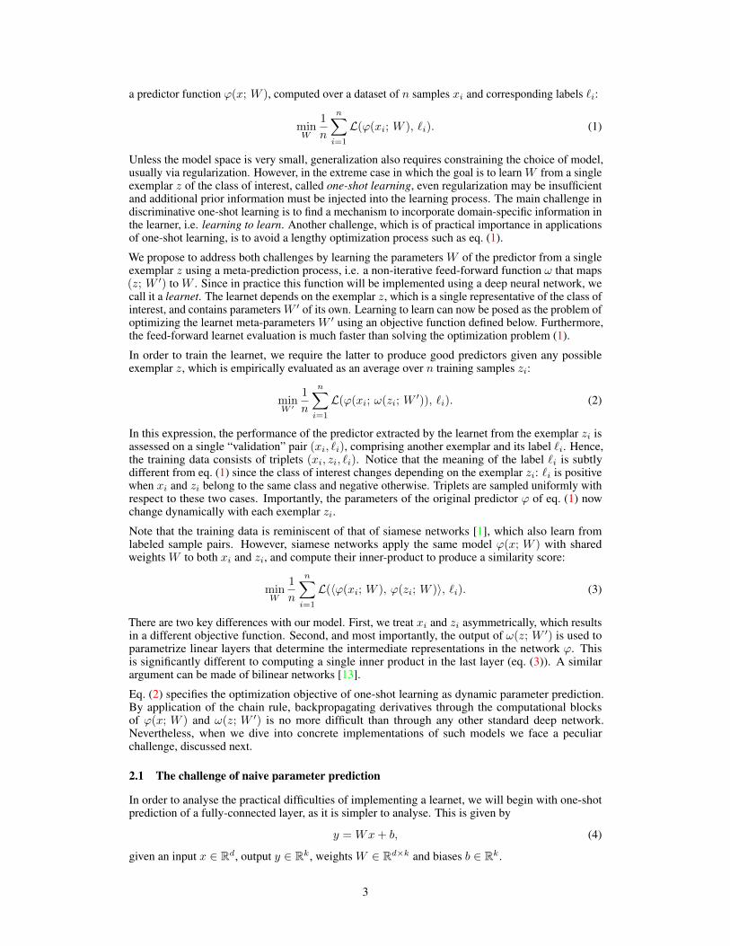
Figure 3: The predicted filters and the output of a dynamic convolutional layer in a single-streamlearnet trained for the OCR task. Different exemplars z define different filters w(z). Applying thefilters of each exemplar to the same input x yields different responses (although in typical operation,the network defined by a single exemplar is applied to many other inputs). Best viewed in colour.

Inner-product (%) Euclidean dist. (%) Weighted `1 dist. (%)Siamese (shared) 48.5 37.3 41.8Siamese (unshared) 47.0 41.0 34.6Siamese (unshared, factorized) 48.4 – 33.6Siamese learnet (shared) 51.0 39.8 31.4Learnet 43.7 36.7 28.6

Table 1: Error rate for character recognition in foreign alphabets (chance is 95%).

The single-stream learnet architecture can be understood to predict a discriminant function from oneexample, and the siamese learnet architecture to predict an embedding function for the comparisonof two images. These two variants demonstrate the versatility of the dynamic convolutional layerfrom eq. (6).

Finally, in order to ensure that any difference in performance is not simply due to the asymmetry ofthe learnet architecture or to the induced filter factorizations (sect. 2.2 and sect. 2.3), we also compareunshared siamese nets, which use distinct parameters for each stream, and factorized siamese nets,where convolutions are replaced by factorized convolutions as in learnet.

3.2 Character recognition in foreign alphabets

This section describes our experiments in one-shot learning on OCR. For this, we use the Omniglotdataset [12], which contains images of handwritten characters from 50 different alphabets. Thesealphabets are divided into 30 background and 20 evaluation alphabets. The associated one-shotlearning problem is to develop a method for determining whether, given any single exemplar of acharacter in an evaluation alphabet, any other image in that alphabet represents the same character ornot. Importantly, all methods are trained using only background alphabets and tested on the evaluationalphabets.

Dataset and evaluation protocol. Character images are resized to 28× 28 pixels in order to be ableto explore efficiently several variants of the proposed architectures. There are exactly 20 sampleimages for each character, and an average of 32 characters per alphabet. The dataset contains a totalof 19,280 images in the background alphabets and 13,180 in the evaluation alphabets.

Algorithms are evaluated on a series of recognition problems. Each recognition problem involvesidentifying the image in a set of 20 that shows the same character as an exemplar image (there isalways exactly one match). All of the characters in a single problem belong to the same alphabet.At test time, given a collection of characters (x1, . . . , xm), the function is evaluated on each pair(z, xi) and the candidate with the highest score is declared the match. In the case of the learnetarchitectures, this can be interpreted as obtaining the parameters W = ω(z;W ′) and then evaluatinga static network ϕ(xi;W ) for each xi.

Architecture. The baseline stream ϕ for the siamese, siamese learnet, and single-stream learnetarchitecture consists of 3 convolutional layers, with 2× 2 max-pooling layers of stride 2 betweenthem. The filter sizes are 5× 5× 1× 16, 5× 5× 16× 64 and 4× 4× 64× 512. For both the siameselearnet and the single-stream learnet, ω consists of the same layers as ϕ, except the number of outputsis 1600 – one for each element of the 64 predicted filters (of size 5× 5). To keep the experimentssimple, we only predict the parameters of one convolutional layer. We conducted cross-validation tochoose the predicted layer and found that the second convolutional layer yields the best results forboth of the proposed variants.

6

Siamese nets have previously been applied to this problem by Koch et al. [9] using much deepernetworks applied to images of size 105 × 105. However, we have restricted this investigation torelatively shallow networks to enable a thorough exploration of the parameter space. A more powerfulalgorithm for one-shot learning, Hierarchical Bayesian Program Learning [12], is able to achievehuman-level performance. However, this approach involves computationally expensive inference attest time, and leverages extra information at training time that describes the strokes drawn by thehuman author.

Learning. Learning involves minimizing the objective function specific to each method (e.g. eq. (2)for learnet and eq. (3) for siamese architectures) and uses stochastic gradient descent (SGD) in allcases. As noted in sect. 2, the objective is obtained by sampling triplets (zi, xi, `i) where exemplarszi and xi are congruous (`i = +1) or incongruous (`i = −1) with 50% probability. We consider100,000 random pairs for training per epoch, and train for 60 epochs. We conducted a randomsearch to find the best hyper-parameters for each algorithm (initial learning rate and geometric decay,standard deviation of Gaussian parameter initialization, and weight decay).

Results and discussion. Tab. 1 shows the classification error obtained using variants of eacharchitecture. A dash indicates a failure to converge given a large range of hyper-parameters. The twolearnet architectures combined with the weighted `1 distance are able to achieve significantly betterresults than other methods. The best architecture reduced the error from 37.3% for a siamese networkwith shared parameters to 28.6% for a single-stream learnet.

While the Euclidean distance gave the best results for siamese networks with shared parameters,better results were achieved by learnets (and siamese networks with unshared parameters) using aweighted `1 distance. In fact, none of the alternative architectures are able to achieve lower errorunder the Euclidean distance than the shared siamese net. The dot product was, in general, lesseffective than the other two metrics.

The introduction of the factorization in the convolutional layer might be expected to improve thequality of the estimated model by reducing the number of parameters, or to worsen it by diminishingthe capacity of the hypothesis space. For this relatively simple task of character recognition, thefactorization did not seem to have a large effect.

3.3 Object tracking

The task of single-target object tracking requires to locate an object of interest in a sequence of videoframes. A video frame can be seen as a collection F = {w1, . . . , wK} of image windows; then, in aone-shot setting, given an exemplar z ∈ F1 of the object in the first frame F1, the goal is to identifythe same window in the other frames F2, . . . ,FM .

Datasets. The method is trained using the ImageNet Large Scale Visual Recognition Challenge2015 [19], with 3,862 videos totalling more than one million annotated frames. Instances of objectsof thirty different classes (mostly vehicles and animals) are annotated throughout each video withbounding boxes. For tracking, instance labels are retained but object class labels are ignored. We use90% of the videos for training, while the other 10% are held-out to monitor validation error duringnetwork training. Testing uses the VOT 2015 benchmark [10].

Architecture. We experiment with siamese and siamese learnet architectures (fig. 2) where thelearnet ω predicts the parameters of the second (dynamic) convolutional layer of the siamese streams.Each siamese stream has five convolutional layers and we test three variants of those: variant (A) hasthe same configuration as AlexNet [11] but with stride 2 in the first layer, and variants (B) and (C)reduce to 50% the number of filters in the first two convolutional layers and, respectively, to 25% and12.5% the number of filters in the last layer.

Training. In order to train the architecture efficiently from many windows, the data is preparedas follows. Given an object bounding box sampled at random, a crop z double the size of that isextracted from the corresponding frame, padding with the average image color when needed. Theborder is included in order to incorporate some visual context around the exemplar object. Next,` ∈ {+1,−1} is sampled at random with 75% probability of being positive. If ` = −1, an image xis extracted by choosing at random a frame that does not contain the object. Otherwise, a secondframe containing the same object and within 50 temporal samples of the first is selected at random.From that, a patch x centered around the object and four times bigger is extracted. In this way, x

7

· · · · · ·

· · · · · ·

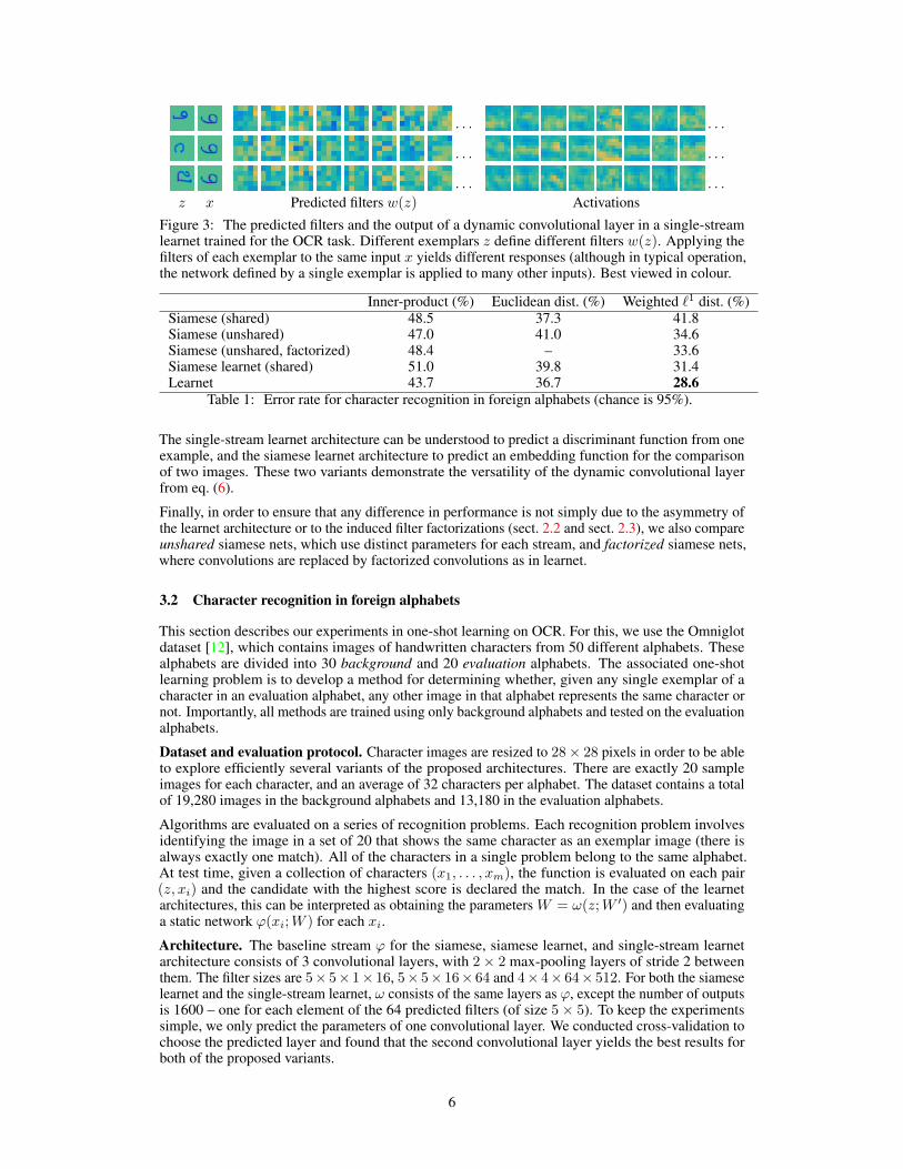
· · · · · ·z x Predicted filters w(z) Activations

Figure 4: The predicted filters and the output of a dynamic convolutional layer in a siamese learnettrained for the object tracking task. Best viewed in colour.

Method Accuracy FailuresSiamese (ϕ=B) 0.465 105Siamese (ϕ=B; unshared) 0.447 131Siamese (ϕ=B; factorized) 0.444 138Siamese learnet (ϕ=B; ω=A) 0.500 87Siamese learnet (ϕ=B; ω=B) 0.497 93DAT [17] 0.442 113SO-DLT [21] 0.540 108

Method Accuracy FailuresSiamese (ϕ=C) 0.466 120Siamese (ϕ=C; factorized) 0.435 132Siamese learnet (ϕ=C; ω=A) 0.483 105Siamese learnet (ϕ=C; ω=C) 0.491 106DSST [2] 0.483 163MEEM [22] 0.458 107MUSTer [6] 0.471 132

Table 2: Tracking accuracy and number of tracking failures in the VOT 2015 Benchmark, as reportedby the toolkit [10]. Architectures are grouped by size of the main network (see text). For each group,the best entry for each column is in bold. We also report the scores of 5 recent trackers.

contains both subwindows that do and do not match z. Images z and x are resized to 127× 127 and255× 255 pixels, respectively, and the triplet (z, x, `) is formed. All 127× 127 subwindows in x areconsidered to not match z except for the central 2× 2 ones when ` = +1.

All networks are trained from scratch using SGD for 50 epoch of 50,000 sample triplets (zi, xi, `i).The multiple windows contained in x are compared to z efficiently by making the comparison layerΓ convolutional (fig. 2), accumulating a logistic loss across spatial locations. The same hyper-parameters (learning rate of 10−2 geometrically decaying to 10−5, weight decay of 0.005, and smallmini-batches of size 8) are used for all experiments, which we found to work well for both the baselineand proposed architectures. The weights are initialized using the improved Xavier [5] method, andwe use batch normalization [7] after all linear layers.

Testing. Adopting the initial crop as exemplar, the object is sought in a new frame within a radius ofthe previous position, proceeding sequentially. This is done by evaluating the pupil net convolutionally,as well as searching at five possible scales in order to track the object through scale space.

Results and discussion. Tab. 3 compares the methods in terms of the official metrics (accuracy andnumber of failures) for the VOT 2015 benchmark [10]. The ranking plot produced by the VOT toolkitis provided in the supplementary material (fig. B.1). From tab. 3, it can be observed that factorizingthe filters in the siamese architecture significantly diminishes its performance, but using a learnet topredict the filters in the factorization recovers this gap and in fact achieves better performance thanthe original siamese net. The performance of the learnet architectures is not adversely affected byusing the slimmer prediction networks B and C (with less channels).

An elementary tracker based on learnet compares favourably against recent tracking systems, whichmake use of different features and online model update strategies: DAT [17], DSST [2], MEEM [22],MUSTer [6] and SO-DLT [21]. SO-DLT in particular is a good example of direct adaptation ofstandard batch deep learning methodology to online learning, as it uses SGD during tracking tofine-tune an ensemble of deep convolutional networks. However, the online adaptation of the modelcomes at a big computational cost and affects the speed of the method, which runs at 5 frames-per-second (FPS) on a GPU. Due to the feed-forward nature of our one-shot learnets, they can trackobjects in real-time at framerates in excess of 60 FPS, while achieving less tracking failures. Weconsider, however, that our implementation serves mostly as a proof-of-concept, using tracking as aninteresting demonstration of one-shot-learning, and is orthogonal to many technical improvementsfound in the tracking literature [10].

8

4 Conclusions

In this work, we have shown that it is possible to obtain the parameters of a deep neural networkusing a single, feed-forward prediction from a second network. This approach is desirable wheniterative methods are too slow, and when large sets of annotated training samples are not available. Wehave demonstrated the feasibility of feed-forward parameter prediction in two demanding one-shotlearning tasks in OCR and visual tracking. Our results hint at a promising avenue of research in“learning to learn” by solving millions of small discriminative problems in an offline phase. Possibleextensions include domain adaptation and sharing a single learnet between different pupil networks.

References

[1] J. Bromley, J. W. Bentz, L. Bottou, I. Guyon, Y. LeCun, C. Moore, E. Säckinger, and R. Shah.Signature verification using a “siamese” time delay neural network. International Journal ofPattern Recognition and Artificial Intelligence, 1993.

[2] M. Danelljan, G. Häger, F. Khan, and M. Felsberg. Accurate scale estimation for robust visualtracking. In BMVC, 2014.

[3] M. Denil, B. Shakibi, L. Dinh, N. de Freitas, et al. Predicting parameters in deep learning. InAdvances in Neural Information Processing Systems, 2013.

[4] H. Fan, Z. Cao, Y. Jiang, Q. Yin, and C. Doudou. Learning deep face representation. arXivCoRR, 2014.

[5] K. He, X. Zhang, S. Ren, and J. Sun. Delving deep into rectifiers: Surpassing human-levelperformance on ImageNet classification. In ICCV, 2015.

[6] Z. Hong, Z. Chen, C. Wang, X. Mei, D. Prokhorov, and D. Tao. Multi-store tracker (MUSTER):A cognitive psychology inspired approach to object tracking. In CVPR, 2015.

[7] S. Ioffe and C. Szegedy. Batch normalization: Accelerating deep network training by reducinginternal covariate shift. arXiv CoRR, 2015.

[8] D. P. Kingma and M. Welling. Auto-encoding variational bayes. arXiv CoRR, 2013.

[9] G. Koch, R. Zemel, and R. Salakhutdinov. Siamese neural networks for one-shot imagerecognition. In ICML 2015 Deep Learning Workshop, 2016.

[10] M. Kristan, J. Matas, A. Leonardis, M. Felsberg, L. Cehovin, G. Fernandez, T. Vojir, G. Hager,G. Nebehay, and R. Pflugfelder. The visual object tracking VOT2015 challenge results. In ICCVWorkshop, 2015.

[11] A. Krizhevsky, I. Sutskever, and G. E. Hinton. ImageNet classification with deep convolutionalneural networks. In Advances in Neural Information Processing Systems, 2012.

[12] B. M. Lake, R. Salakhutdinov, and J. B. Tenenbaum. Human-level concept learning throughprobabilistic program induction. Science, 350(6266):1332–1338, 2015.

[13] T.-Y. Lin, A. RoyChowdhury, and S. Maji. Bilinear CNN models for fine-grained visualrecognition. In ICCV, 2015.

[14] T. Malisiewicz, A. Gupta, and A. A. Efros. Ensemble of exemplar-SVMs for object detectionand beyond. In ICCV, 2011.

[15] H. Nam and B. Han. Learning multi-domain convolutional neural networks for visual tracking.arXiv CoRR, 2015.

[16] O. M. Parkhi, A. Vedaldi, and A. Zisserman. Deep face recognition. BMVC, 2015.

[17] H. Possegger, T. Mauthner, and H. Bischof. In defense of color-based model-free tracking. InCVPR, 2015.

[18] D. J. Rezende, S. Mohamed, I. Danihelka, K. Gregor, and D. Wierstra. One-shot generalizationin deep generative models. arXiv CoRR, 2016.

[19] O. Russakovsky, J. Deng, H. Su, J. Krause, S. Satheesh, S. Ma, Z. Huang, A. Karpathy,A. Khosla, M. Bernstein, A. C. Berg, and L. Fei-Fei. ImageNet Large Scale Visual RecognitionChallenge. International Journal of Computer Vision, 2015.

9

[20] R. Socher, M. Ganjoo, C. D. Manning, and A. Ng. Zero-shot learning through cross-modaltransfer. In Advances in Neural Information Processing Systems, 2013.

[21] N. Wang, S. Li, A. Gupta, and D.-Y. Yeung. Transferring rich feature hierarchies for robustvisual tracking. arXiv CoRR, 2015.

[22] J. Zhang, S. Ma, and S. Sclaroff. MEEM: Robust tracking via multiple experts using entropyminimization. In ECCV. 2014.

A Basis filters

This appendix provides an additional interpretation for the role of the predicted filters in a factorizedconvolutional layer (Section 2.3).

To make the presentation succint, we will use a notation that is slightly different from the main text.Let x be a tensor of activations, then xi denotes channel i of x. If a is a multi-channel filter, then aijdenotes the filter for output channel i and input channel j. That is, if a is m× n× p× q then aij ism× n for i ∈ [p], j ∈ [q]. The set {1, . . . , n} is denoted [n].

The factorised convolution isy = Ax = M ′WMx . (9)

where M and M ′ are pixel-wise projections and W is a diagonal convolution. While a generalconvolution computes

(Av)i =∑

j aij ∗ vj (10)

where each aij is a single-channel filter, a diagonal convolution computes

(Wv)i = wi ∗ vi (11)

where each wi is a single-channel filter, and a pixel-wise projection computes

(Mv)i =∑

j mijvj (12)

where each mij is a scalar.

Let q be the number of channels of x, let p be the number of channels of y and let r be the number ofchannels of the intermediate activations. Combining the above gives

(WMx)k = wk ∗(∑

j∈[q]mkjxj

)=∑

j∈[q]mkjwk ∗ xj (13)

(M ′WMx)i =∑

k∈[r]m′ik

(∑j∈[q]mkjwk ∗ xj

)=∑

j∈[q]

(∑k∈[r]m

′ikmkjwk

)∗ xj . (14)

This is therefore equivalent to a general convolution y = Ax where each filter aij is a combination ofr single-channel basis filters wk

aij =∑

k∈[r]m′ikmkjwk (15)

The predictions used in the dynamic convolution (Section 2.3) essentially modify these r basis filters.

10

B Additional results on object tracking

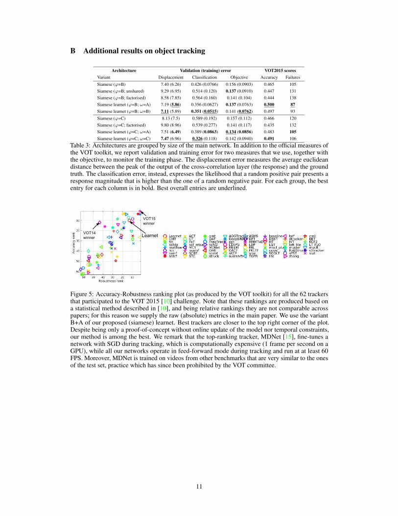
Architecture Validation (training) error VOT2015 scoresVariant Displacement Classification Objective Accuracy Failures

Siamese (ϕ=B) 7.40 (6.26) 0.426 (0.0766) 0.156 (0.0903) 0.465 105Siamese (ϕ=B; unshared) 9.29 (6.95) 0.514 (0.120) 0.137 (0.0910) 0.447 131Siamese (ϕ=B; factorised) 8.58 (7.85) 0.564 (0.160) 0.141 (0.104) 0.444 138Siamese learnet (ϕ=B; ω=A) 7.19 (5.86) 0.356 (0.0627) 0.137 (0.0763) 0.500 87Siamese learnet (ϕ=B; ω=B) 7.11 (5.89) 0.351 (0.0515) 0.141 (0.0762) 0.497 93

Siamese (ϕ=C) 8.13 (7.5) 0.589 (0.192) 0.157 (0.112) 0.466 120Siamese (ϕ=C; factorised) 9.80 (8.96) 0.539 (0.277) 0.141 (0.117) 0.435 132Siamese learnet (ϕ=C; ω=A) 7.51 (6.49) 0.389 (0.0863) 0.134 (0.0856) 0.483 105Siamese learnet (ϕ=C; ω=C) 7.47 (6.96) 0.326 (0.118) 0.142 (0.0940) 0.491 106

Table 3: Architectures are grouped by size of the main network. In addition to the official measures ofthe VOT toolkit, we report validation and training error for two measures that we use, together withthe objective, to monitor the training phase. The displacement error measures the average euclideandistance between the peak of the output of the cross-correlation layer (the response) and the groundtruth. The classification error, instead, expresses the likelihood that a random positive pair presents aresponse magnitude that is higher than the one of a random negative pair. For each group, the bestentry for each column is in bold. Best overall entries are underlined.

LearnetVOT14winner

VOT15winner

Figure 5: Accuracy-Robustness ranking plot (as produced by the VOT toolkit) for all the 62 trackersthat participated to the VOT 2015 [10] challenge. Note that these rankings are produced based ona statistical method described in [10], and being relative rankings they are not comparable acrosspapers; for this reason we supply the raw (absolute) metrics in the main paper. We use the variantB+A of our proposed (siamese) learnet. Best trackers are closer to the top right corner of the plot.Despite being only a proof-of-concept without online update of the model nor temporal constraints,our method is among the best. We remark that the top-ranking tracker, MDNet [15], fine-tunes anetwork with SGD during tracking, which is computationally expensive (1 frame per second on aGPU), while all our networks operate in feed-forward mode during tracking and run at at least 60FPS. Moreover, MDNet is trained on videos from other benchmarks that are very similar to the onesof the test set, practice which has since been prohibited by the VOT committee.

11

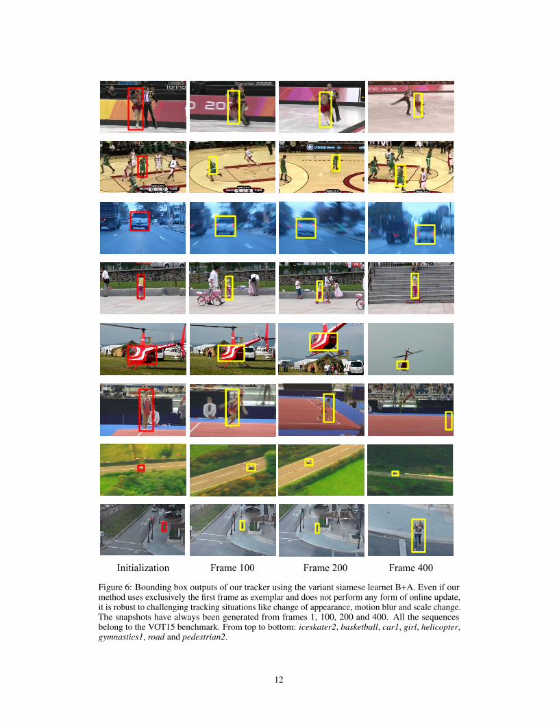
Initialization Frame 100 Frame 200 Frame 400

Figure 6: Bounding box outputs of our tracker using the variant siamese learnet B+A. Even if ourmethod uses exclusively the first frame as exemplar and does not perform any form of online update,it is robust to challenging tracking situations like change of appearance, motion blur and scale change.The snapshots have always been generated from frames 1, 100, 200 and 400. All the sequencesbelong to the VOT15 benchmark. From top to bottom: iceskater2, basketball, car1, girl, helicopter,gymnastics1, road and pedestrian2.

12