learning ev alua tion functions - robotics institute · learning ev alua tion functions f or global...
TRANSCRIPT

Learning Evaluation Functions
for Global Optimization
Justin Andrew Boyan
August 1, 1998CMU-CS-98-152
School of Computer ScienceCarnegie Mellon University
Pittsburgh, PA 15213
A dissertation submitted in partial ful�llment of the
requirements for the degree of Doctor of Philosophy
Thesis committee:Andrew W. Moore (co-chair)Scott E. Fahlman (co-chair)
Tom M. MitchellThomas G. Dietterich, Oregon State University
Copyright c 1998, Justin Andrew Boyan
Support for this work has come from the National Defense Science and Engineering Graduatefellowship; National Science Foundation grant IRI-9214873; the Engineering Design Research Center(EDRC), an NSF Engineering Research Center; the Pennsylvania Space Grant fellowship; and theNASA Graduate Student Researchers Program fellowship. The views and conclusions contained inthis document are those of the author and should not be interpreted as representing the o�cialpolicies, either expressed or implied, of ARPA, NSF, NASA, or the U.S. government.

Keywords: Machine learning, combinatorial optimization, reinforcement learn-ing, temporal di�erence learning, evaluation functions, local search, heuristic search,simulated annealing, value function approximation, neuro-dynamic programming,Boolean satis�ability, radiotherapy treatment planning, channel routing, bin-packing,Bayes network learning, production scheduling

1
Abstract
In complex sequential decision problems such as scheduling factory production, plan-ning medical treatments, and playing backgammon, optimal decision policies are ingeneral unknown, and it is often di�cult, even for human domain experts, to manuallyencode good decision policies in software. The reinforcement-learning methodologyof \value function approximation" (VFA) o�ers an alternative: systems can learne�ective decision policies autonomously, simply by simulating the task and keepingstatistics on which decisions lead to good ultimate performance and which do not.This thesis advances the state of the art in VFA in two ways.
First, it presents three new VFA algorithms, which apply to three di�erent re-stricted classes of sequential decision problems: Grow-Support for deterministic prob-lems, ROUT for acyclic stochastic problems, and Least-Squares TD(�) for �xed-policyprediction problems. Each is designed to gain robustness and e�ciency over currentapproaches by exploiting the restricted problem structure to which it applies.
Second, it introduces STAGE, a new search algorithm for general combinatorialoptimization tasks. STAGE learns a problem-speci�c heuristic evaluation function asit searches. The heuristic is trained by supervised linear regression or Least-SquaresTD(�) to predict, from features of states along the search trajectory, how well a fastlocal search method such as hillclimbing will perform starting from each state. Searchproceeds by alternating between two stages: performing the fast search to gather newtraining data, and following the learned heuristic to identify a promising new startstate.
STAGE has produced good results (in some cases, the best results known) ona variety of combinatorial optimization domains, including VLSI channel routing,Bayes net structure-�nding, bin-packing, Boolean satis�ability, radiotherapy treat-ment planning, and geographic cartogram design. This thesis describes the resultsin detail, analyzes the reasons for and conditions of STAGE's success, and placesSTAGE in the context of four decades of research in local search and evaluation func-tion learning. It provides strong evidence that reinforcement learning methods canbe e�cient and e�ective on large-scale decision problems.

2

3
Dedication
To my grandfather,
Ara Boyan, 1906{93

4

5
Acknowledgments
This dissertation represents the culmination of my six years of graduate study at
CMU and of my formal education as a whole. Many, many people helped me achieve
this goal, and I would like to thank a few of them in writing. Readers who disdain
sentimentality may wish to turn the page now!
First, I thank my primary advisor, Andrew Moore. Since his arrival at CMU one
year after mine, Andrew has been a mentor, role model, collaborator, and friend. No
one else I know has such a clear grasp of what really matters in machine learning and
in computer science as a whole. His long-term vision has helped keep my research
focused, and his technical brilliance has helped keep it sound. Moreover, his patience,
ability to listen, and innate personal generosity will always inspire me. Unlike the
stereotypical professor who has his graduate students do the work and then helps
himself to the credit, Andrew has a way of listening to your half-baked brainstorming,
reformulating it into a sensible idea, and then convincing you the idea was yours all
along. I feel very lucky indeed to have been his �rst Ph.D. student!
My other three committee members have also been extremely helpful. Scott
Fahlman, my co-advisor, helped teach me how to cut to the heart of an idea and
how to present it clearly. When my progress was slow, Scott always encouraged me
with the right blend of carrots and sticks. Tom Mitchell enthusiastically supported
my ideas while at the same time asking good, tough questions. Finally, Tom Diet-
terich has been a wonderful external committeemember|from the early stages, when
his doubts about my approach served as a great motivating challenge, until the very
end, when his comments on this document were especially thorough and helpful.
Three friends at CMU|Michael Littman, Marc Ringuette, and Je� Schneider|
also contributed immeasurably to my graduate education by being my regular part-
ners for brainstorming and arguing about research ideas. I credit Michael with in-
troducing me to the culture of computer science research, and also thank him for his
extensive comments on a thesis draft.
Only in the past year or two have I come to appreciate how amazing a place CMU
is to do research. I would like to thank all my friends in the Reinforcement Learning
group here, especially Leemon Baird, Shumeet Baluja, Rich Caruana, Scott Davies,
Frank Dellaert, Kan Deng, Geo� Gordon, Thorsten Joachims, Andrew McCallum,
Peter Stone, Astro Teller, and Belinda Thom. Special thanks also go to my o�cemates
over the years, including Lin Chase, Fabio Cozman, John Hancock, and Jennie Kay.
The CMU faculty, too, could not have been more supportive. Besides my commit-
tee members, the following professors all made time to discuss my thesis and assist

6
my research: Avrim Blum, Jon Cagan, Paul Heckbert, Jack Mostow, Steven Rudich,
Rob Rutenbar, Sebastian Thrun, Mike Trick, and Manuela Veloso. I would also like
to thank the entire Robotics Institute for allowing me access to over one hundred of
their workstations for my 40,000+ computational experiments!
The third major part of what makes the CMU environment so amazing is the
excellence of the department administration. I would particularly like to thank Sharon
Burks, Catherine Copetas, Jean Harpley, and Karen Olack, who made every piece of
paperwork a pleasure (well, nearly), and who manage to run a big department with
a personal touch.
Outside CMU, I would like to thank the greater reinforcement-learning and machine-
learning communities|especially Chris Atkeson, Andy Barto, Wray Buntine, Tom
Dietterich, Leslie Kaelbling, Pat Langley, Sridhar Mahadevan, Satinder Singh, Rich
Sutton, and Gerry Tesauro. These are leaders of the �eld, yet they are all wonderfully
down-to-earth and treat even greenhorns like myself as colleagues.
Finally, I thank the following institutions that provided �nancial support for my
graduate studies: the Winston Churchill Foundation of the United States (1991{
92); the National Defense Science and Engineering Graduate fellowship (1992{95);
National Science Foundation grant IRI-9214873 (1992{94); the Engineering Design
Research Center (EDRC), an NSF Engineering Research Center (1995{96); the Penn-
sylvania Space Grant fellowship (1995{96); and the NASA Graduate Student Re-
searchers Program (GSRP) fellowship (1996{98). I thank Steve Chien at JPL for
sponsoring my GSRP fellowship.
* * *
On a more personal level, I would like to thank my closest friends during graduate
school, who got me through all manner of trials and tribulations: Marc Ringuette,
Michael Littman, Kelly Amienne, Zoran Popovi�c, Lisa Falenski, and Je� Schneider.
Peter Stone deserves special thanks for making possible my trips to Brazil and Japan
in 1997. I also thank Erik Winfree and all my CTY friends in the Mattababy Group
for their constant friendship.
Second, I would like to thank the teachers and professors who have guided and
inspired me throughout my education, including Barbara Jewett, Paul Sally, Stuart
Kurtz, John MacAloon, and Charles Martin.
Finally, I would like to thank the two best teachers I know: my parents, Steve
and Kitty Boyan. They taught me the values of education and thoughtfulness, of
moderation and balance, and of love for all people and life. To thank them properly|
for all the opportunities and freedoms they provided for me, and for all their wisdom
and love|would �ll the pages of another book as long as this one.
7
Table of Contents
1 Introduction . . . . . . . . . . . . . . . . . . . . . . . . . . . . . . . . . 11
1.1 Motivation: Learning Evaluation Functions . . . . . . . . . . . . . . . 11
1.2 The Promise of Reinforcement Learning . . . . . . . . . . . . . . . . 12
1.3 Outline of the Dissertation . . . . . . . . . . . . . . . . . . . . . . . . 14
2 Learning Evaluation Functions for Sequential Decision Making 17
2.1 Value Function Approximation (VFA) . . . . . . . . . . . . . . . . . . 17
2.1.1 Markov Decision Processes . . . . . . . . . . . . . . . . . . . . 17
2.1.2 VFA Literature Review . . . . . . . . . . . . . . . . . . . . . . 20
2.1.3 Working Backwards . . . . . . . . . . . . . . . . . . . . . . . . 24
2.2 VFA in Deterministic Domains: \Grow-Support" . . . . . . . . . . . 25
2.3 VFA in Acyclic Domains: \ROUT" . . . . . . . . . . . . . . . . . . . 27
2.3.1 Task 1: Stochastic Path Length Prediction . . . . . . . . . . . 31
2.3.2 Task 2: A Two-Player Dice Game . . . . . . . . . . . . . . . . 31
2.3.3 Task 3: Multi-armed Bandit Problem . . . . . . . . . . . . . . 32
2.3.4 Task 4: Scheduling a Factory Production Line . . . . . . . . . 35
2.4 Discussion . . . . . . . . . . . . . . . . . . . . . . . . . . . . . . . . . 38
3 Learning Evaluation Functions for Global Optimization . . . . 41
3.1 Introduction . . . . . . . . . . . . . . . . . . . . . . . . . . . . . . . . 41
3.1.1 Global Optimization . . . . . . . . . . . . . . . . . . . . . . . 41
3.1.2 Local Search . . . . . . . . . . . . . . . . . . . . . . . . . . . . 43
3.1.3 Using Additional State Features . . . . . . . . . . . . . . . . . 44
3.2 The \STAGE" Algorithm . . . . . . . . . . . . . . . . . . . . . . . . 47
3.2.1 Learning to Predict . . . . . . . . . . . . . . . . . . . . . . . . 47
3.2.2 Using the Predictions . . . . . . . . . . . . . . . . . . . . . . . 49
3.3 Illustrative Examples . . . . . . . . . . . . . . . . . . . . . . . . . . . 51
3.3.1 1-D Wave Function . . . . . . . . . . . . . . . . . . . . . . . . 51
3.3.2 Bin-packing . . . . . . . . . . . . . . . . . . . . . . . . . . . . 54
3.4 Theoretical and Computational Issues . . . . . . . . . . . . . . . . . . 55
3.4.1 Choosing � . . . . . . . . . . . . . . . . . . . . . . . . . . . . 57
3.4.2 Choosing the Features . . . . . . . . . . . . . . . . . . . . . . 63
3.4.3 Choosing the Fitter . . . . . . . . . . . . . . . . . . . . . . . . 64
3.4.4 Discussion . . . . . . . . . . . . . . . . . . . . . . . . . . . . . 68

8 Table of Contents|Continued
4 STAGE: Empirical Results . . . . . . . . . . . . . . . . . . . . . . . . 694.1 Experimental Methodology . . . . . . . . . . . . . . . . . . . . . . . . 70
4.1.1 Reference Algorithms . . . . . . . . . . . . . . . . . . . . . . . 704.1.2 How the Results are Tabulated . . . . . . . . . . . . . . . . . 71
4.2 Bin-packing . . . . . . . . . . . . . . . . . . . . . . . . . . . . . . . . 724.3 VLSI Channel Routing . . . . . . . . . . . . . . . . . . . . . . . . . . 794.4 Bayes Network Learning . . . . . . . . . . . . . . . . . . . . . . . . . 844.5 Radiotherapy Treatment Planning . . . . . . . . . . . . . . . . . . . . 904.6 Cartogram Design . . . . . . . . . . . . . . . . . . . . . . . . . . . . . 934.7 Boolean Satis�ability . . . . . . . . . . . . . . . . . . . . . . . . . . . 95
4.7.1 WALKSAT . . . . . . . . . . . . . . . . . . . . . . . . . . . . 954.7.2 Experimental Setup . . . . . . . . . . . . . . . . . . . . . . . . 974.7.3 Main Results . . . . . . . . . . . . . . . . . . . . . . . . . . . 994.7.4 Follow-up Experiments . . . . . . . . . . . . . . . . . . . . . . 101
4.8 Boggle Board Setup . . . . . . . . . . . . . . . . . . . . . . . . . . . . 1024.9 Discussion . . . . . . . . . . . . . . . . . . . . . . . . . . . . . . . . . 106
5 STAGE: Analysis . . . . . . . . . . . . . . . . . . . . . . . . . . . . . . . 1075.1 Explaining STAGE's Success . . . . . . . . . . . . . . . . . . . . . . . 107
5.1.1 ~V � versus Other Secondary Policies . . . . . . . . . . . . . . . 1085.1.2 ~V � versus Simple Smoothing . . . . . . . . . . . . . . . . . . . 1105.1.3 Learning Curves for Channel Routing . . . . . . . . . . . . . . 1135.1.4 STAGE's Failure on Boggle Setup . . . . . . . . . . . . . . . . 117
5.2 Empirical Studies of Parameter Choices . . . . . . . . . . . . . . . . . 1175.2.1 Feature Sets . . . . . . . . . . . . . . . . . . . . . . . . . . . . 1185.2.2 Fitters . . . . . . . . . . . . . . . . . . . . . . . . . . . . . . . 1245.2.3 Policy � . . . . . . . . . . . . . . . . . . . . . . . . . . . . . . 1275.2.4 Exploration/Exploitation . . . . . . . . . . . . . . . . . . . . . 1305.2.5 Patience and ObjBound . . . . . . . . . . . . . . . . . . . . . 132
5.3 Discussion . . . . . . . . . . . . . . . . . . . . . . . . . . . . . . . . . 133
6 STAGE: Extensions . . . . . . . . . . . . . . . . . . . . . . . . . . . . . 1376.1 Using TD(�) to learn V � . . . . . . . . . . . . . . . . . . . . . . . . . 137
6.1.1 TD(�): Background . . . . . . . . . . . . . . . . . . . . . . . 1386.1.2 The Least-Squares TD(�) Algorithm . . . . . . . . . . . . . . 1426.1.3 LSTD(�) as Model-Based TD(�) . . . . . . . . . . . . . . . . 1446.1.4 Empirical Comparison of TD(�) and LSTD(�) . . . . . . . . . 1476.1.5 Applying LSTD(�) in STAGE . . . . . . . . . . . . . . . . . . 150
6.2 Transfer . . . . . . . . . . . . . . . . . . . . . . . . . . . . . . . . . . 1536.2.1 Motivation . . . . . . . . . . . . . . . . . . . . . . . . . . . . . 153
Table of Contents|Continued 9
6.2.2 X-STAGE: A Voting Algorithm for Transfer . . . . . . . . . . 1556.2.3 Experiments . . . . . . . . . . . . . . . . . . . . . . . . . . . . 156
6.3 Discussion . . . . . . . . . . . . . . . . . . . . . . . . . . . . . . . . . 159
7 Related Work . . . . . . . . . . . . . . . . . . . . . . . . . . . . . . . . 1617.1 Adaptive Multi-Restart Techniques . . . . . . . . . . . . . . . . . . . 1617.2 Reinforcement Learning for Optimization . . . . . . . . . . . . . . . . 1647.3 Rollouts and Learning for AI Search . . . . . . . . . . . . . . . . . . 1677.4 Genetic Algorithms . . . . . . . . . . . . . . . . . . . . . . . . . . . . 1697.5 Discussion . . . . . . . . . . . . . . . . . . . . . . . . . . . . . . . . . 171
8 Conclusions . . . . . . . . . . . . . . . . . . . . . . . . . . . . . . . . . . 1738.1 Contributions . . . . . . . . . . . . . . . . . . . . . . . . . . . . . . . 1738.2 Future Directions . . . . . . . . . . . . . . . . . . . . . . . . . . . . . 175
8.2.1 Extending STAGE . . . . . . . . . . . . . . . . . . . . . . . . 1758.2.2 Other Uses of VFA for Optimization . . . . . . . . . . . . . . 1778.2.3 Direct Meta-Optimization . . . . . . . . . . . . . . . . . . . . 178
8.3 Concluding Remarks . . . . . . . . . . . . . . . . . . . . . . . . . . . 180
A Proofs . . . . . . . . . . . . . . . . . . . . . . . . . . . . . . . . . . . . . 181A.1 The Best-So-Far Procedure Is Markovian . . . . . . . . . . . . . . . . 181A.2 Least-Squares TD(1) Is Equivalent to Linear Regression . . . . . . . . 185
B Simulated Annealing . . . . . . . . . . . . . . . . . . . . . . . . . . . . 187B.1 Annealing Schedules . . . . . . . . . . . . . . . . . . . . . . . . . . . 187B.2 The \Modi�ed Lam" Schedule . . . . . . . . . . . . . . . . . . . . . . 188B.3 Experiments . . . . . . . . . . . . . . . . . . . . . . . . . . . . . . . . 191
C Implementation Details of Problem Instances . . . . . . . . . . . 195C.1 Bin-packing . . . . . . . . . . . . . . . . . . . . . . . . . . . . . . . . 195C.2 VLSI Channel Routing . . . . . . . . . . . . . . . . . . . . . . . . . . 196C.3 Bayes Network Learning . . . . . . . . . . . . . . . . . . . . . . . . . 197C.4 Radiotherapy Treatment Planning . . . . . . . . . . . . . . . . . . . . 197C.5 Cartogram Design . . . . . . . . . . . . . . . . . . . . . . . . . . . . . 199C.6 Boolean Satis�ability . . . . . . . . . . . . . . . . . . . . . . . . . . . 199
References . . . . . . . . . . . . . . . . . . . . . . . . . . . . . . . . . . . . 201

10

11
Chapter 1
Introduction
In the industrial age, humans delegated physical labor to machines. Now, in the
information age, we are increasingly delegating mental labor, charging computers
with such tasks as controlling tra�c signals, scheduling factory production, planning
medical treatments, allocating investment portfolios, routing data through commu-
nications networks, and even playing expert-level backgammon or chess. Such tasks
are di�cult sequential decision problems:
� the task calls not for a single decision, but rather for a whole series of decisions
over time;
� the outcome of any decision may depend on random environmental factors be-
yond the computer's control; and
� the ultimate objective|measured in terms of tra�c ow, patient health, busi-
ness pro�t, or game victory|depends in a complicated way on many interacting
decisions and their random outcomes.
In such complex problems, optimal decision policies are in general unknown, and it is
often di�cult, even for human domain experts, to manually encode even reasonably
good decision policies in software. A growing body of research in Arti�cial Intelligence
suggests the following alternative methodology:
A decision-making algorithm can autonomously learn e�ective
policies for sequential decision tasks, simply by simulating the
task and keeping statistics on which decisions tend to lead to
good ultimate performance and which do not.
The �eld of reinforcement learning, to which this thesis contributes, de�nes a princi-
pled foundation for this methodology.
1.1 Motivation: Learning Evaluation Functions
In Arti�cial Intelligence, the fundamental data structure for decision-making in large
state spaces is the evaluation function. Which state should be visited next in the
12 INTRODUCTION
search for a better, nearer, cheaper goal state? The evaluation function maps features
of each state to a real value that assesses the state's promise. For example, in the do-
main of chess, a classic evaluation function is obtained by summingmaterial advantage
weighted by 1 for pawns, 3 for bishops and knights, 5 for rooks, and 9 for queens. The
choice of evaluation function \critically determines search results" [Nilsson 80, p.74]
in popular algorithms for planning and control (A�), game-playing (alpha-beta), and
combinatorial optimization (hillclimbing, simulated annealing).
Evaluation functions have generally been designed by human domain experts.
The weights f1,3,3,5,9g in the chess evaluation function given above summarize the
judgment of generations of chess players. IBM's Deep Blue chess computer, which
defeated world champion Garry Kasparov in a 1997 match, used an evaluation func-
tion of over 8000 tunable parameters|the values of which were set initially by an
automatic procedure, but later carefully hand-tuned under the guidance of a human
grandmaster [Hsu et al. 90, Campbell 98]. Similar tuning occurs in combinatorial
optimization domains such as the Traveling Salesperson Problem [Lin and Kernighan
73] and VLSI circuit design tasks [Wong et al. 88]. In such domains the state space
consists of legal candidate solutions, and the domain's objective function|the func-
tion that evaluates the quality of a �nal solution|can itself serve as an evaluation
function to guide search. However, if the objective function has many local optima
or regions of constant value (plateaus) with respect to the available search moves,
then it will not be e�ective as an evaluation function. Thus, to get good optimization
results, engineers often spend considerable e�ort tweaking the coe�cients of penalty
terms and other additions to their objective function; I cite several examples of this
in Chapter 3. Clearly, automatic methods for building evaluation functions o�er
the potential both to save human e�ort and to optimize search performance more
e�ectively.
1.2 The Promise of Reinforcement Learning
Reinforcement learning (RL) provides a solid foundation for learning evaluation func-
tions for sequential decision problems. Standard RL methods assume that the prob-
lem can be formalized as a Markov decision process (MDP), a model of controllable
dynamic systems used widely in control theory, arti�cial intelligence, and operations
research [Puterman 94]. I describe the MDP model in detail in Chapter 2. The key
fact about this model is that for any MDP, there exists a special evaluation function
known as the optimal value function. Denoted by V �(x), the optimal value function
predicts the expected long-term reward available from each state x when all future
decisions are made optimally. V � is an ideal evaluation function: a greedy one-step

x1.2 THE PROMISE OF REINFORCEMENT LEARNING 13
lookahead search based on V � identi�es precisely the optimal long-term decision to
make at each state. The problem, then, becomes how to compute V �.
Algorithms for computing V � are well understood in the case where the MDP state
space is relatively small (say, fewer than 107 discrete states), so that V � can be imple-
mented as a lookup table. In small MDPs, if we have access to the transition model
which tells us the distribution of successor states that will result from applying a given
action in a given state, then V � may be calculated exactly by a variety of classical algo-
rithms such as dynamic programming or linear programming [Puterman 94]. In small
MDPs where the explicit transition model is not available, we must build V � from
sample trajectories generated by direct interaction with a simulation of the process; in
this case, recently discovered reinforcement learning methods such as TD(�) [Sutton
88], Q-learning [Watkins 89], and Prioritized Sweeping [Moore and Atkeson 93] apply.
These algorithms apply dynamic programming in an asynchronous, incremental way,
but under suitable conditions can still be shown to converge to V � [Bertsekas and
Tsitsiklis 96,Littman and Szepesv�ari 96].
The situation is very di�erent for large-scale decision tasks, such as the trans-
portation and medical domains mentioned at the start of this chapter. These tasks
have high-dimensional state spaces, so enumerating V � in a table is intractable|a
problem known as the \curse of dimensionality" [Bellman 57]. One approach to es-
caping this curse is to approximate V � compactly using a function approximator such
as linear regression or a neural network. The combination of reinforcement learning
and function approximation, known as neuro-dynamic programming [Bertsekas and
Tsitsiklis 96] or value function approximation [Boyan et al. 95], has produced several
notable successes on such problems as backgammon [Tesauro 92,Boyan 92], job-shop
scheduling [Zhang and Dietterich 95], and elevator control [Crites and Barto 96].
However, these implementations are extremely computationally intensive, requiring
many thousands or even millions of simulated trajectories to reach top performance.
Furthermore, when general function approximators are used instead of lookup ta-
bles, the convergence proofs for nearly all dynamic programming and reinforcement
learning algorithms fail to carry through [Boyan and Moore 95,Bertsekas 95,Baird
95,Gordon 95]. Perhaps the strongest convergence result for value function approx-
imation to date is the following [Tsitsiklis and Roy 96]: for an MDP with a �xed
decision-making policy, the TD(�) algorithm may be used to calculate an accurate
linear approximation to the value function. Though its assumption of a �xed policy
is quite limiting, this theorem nonetheless applies to the learning done by STAGE, a
practical algorithm for global optimization introduced in this dissertation.

14 INTRODUCTION
1.3 Outline of the Dissertation
This thesis aims to advance the state of the art in value function approximation for
large, practical sequential decision tasks. It addresses two questions:
1. Can we devise new methods for value function approximation that are robust
and e�cient?
2. Can we apply the currently available convergence results to practical problems?
Both questions are answered in the a�rmative:
1. I discuss three new algorithms for value function approximation, which apply
to three di�erent restricted classes of Markov decision processes: Grow-Support
for large deterministic MDPs (x2.2), ROUT for large acyclic MDPs (x2.3), and
Least-Squares TD(�) for large Markov chains (x6.1). Each is designed to gain
robustness and e�ciency by exploiting the restricted MDP structure to which
it applies.
2. I introduce STAGE, a new reinforcement learning algorithm designed specif-
ically for large-scale global optimization tasks. In STAGE, commonly applied
local optimization algorithms such as stochastic hillclimbing are viewed as in-
ducing �xed decision policies on an MDP. Given that view, TD(�) or supervised
learning may be applied to learn an approximate value function for the policy.
STAGE then exploits the learned value function to improve optimization per-
formance in real time.
The thesis is organized as follows:
Chapter 2 presents formal de�nitions and notation for Markov decision processes
and value function approximation. It then summarizes Grow-Support and
ROUT, algorithms which learn to approximate V � in deterministic and acyclic
MDPs, respectively. Both these algorithms build V � strictly backward from the
goal, even when given only a forward simulation model, as is usually the case.
These algorithms have been presented previously [Boyan and Moore 95,Boyan
and Moore 96], but this chapter o�ers a new uni�ed discussion of both algo-
rithms and new results and analysis for ROUT.
Chapter 3 introduces STAGE, the algorithm which is the main contribution of this
dissertation [Boyan and Moore 97,Boyan and Moore 98]. STAGE is a practical
method for applying value function approximation to arbitrary large-scale global
optimization problems. This chapter motivates and describes the algorithm and
discusses issues of theoretical soundness and computational e�ciency.
x1.3 OUTLINE OF THE DISSERTATION 15
Chapter 4 presents empirical results with STAGE on seven large-scale optimization
domains: bin-packing, channel routing, Bayes net structure-�nding, radiother-
apy treatment planning, cartogram design, Boolean formula satis�ability, and
Boggle board setup. The results show that on a wide range of problems, STAGE
learns e�ciently, e�ectively, and with minimal need for problem-speci�c param-
eter tuning.
Chapter 5 analyzes STAGE's success, giving evidence that reinforcement learning
is indeed responsible for the observed improvements in performance. The sensi-
tivity of the algorithm to various user choices, such as the feature representation
and function approximator, and to various algorithmic choices, such as when to
end a trial and how to begin a new one, is tested empirically.
Chapter 6 o�ers two signi�cant investigations beyond the basic STAGE algorithm.
In Section 6.1, I describe a least-squares implementation of TD(�), which gen-
eralizes both standard supervised linear regression and earlier results on least-
squares TD(0) [Bradtke and Barto 96]. In Section 6.2, I discuss ways of trans-
ferring knowledge learned by STAGE from already-solved instances to novel
similar instances, with the goal of saving training time.
Chapter 7 reviews the relevant work from the optimization and AI literatures, sit-
uating STAGE at the con uence of adaptive multi-start local search methods,
reinforcement learning methods, genetic algorithms, and evaluation function
learning techniques for game-playing and problem-solving search.
Chapter 8 concludes with a summary of the thesis contributions and a discussion
of the many directions for future research in value function approximation for
optimization.

16
17
Chapter 2
Learning Evaluation Functions for Sequential
Decision Making
Given only a simulator for a complex task and a measure of overall cumulative per-
formance, how can we e�ciently build an evaluation function which enables optimal
or near-optimal decisions to be made at every choice point? This chapter discusses
approaches based on the formalism of Markov decision processes and value functions.
After introducing the notation which will be used throughout this dissertation, I give
a review of the literature on value function approximation. I then discuss two original
approaches, Grow-Support and ROUT, for approximating value functions robustly in
certain restricted problem classes.
2.1 Value Function Approximation (VFA)
The optimal value function is an evaluation function which encapsulates complete
knowledge of the best expected search outcome attainable from each state:
V �(x) = the expected long-term reward starting from x, assuming optimal decisions.(2.1)
Such an evaluation function is ideal in that a greedy local search with respect to V �
will always make the globally optimal move. In this section, I formalize the above
de�nition, review the literature on computing V �(x), and motivate a new class of
approximation algorithms for this problem based on working backwards.
2.1.1 Markov Decision Processes
Formally, let our search space be represented as a Markov decision process (MDP),
de�ned by
� a �nite set of states X, including a set of start states S � X;
� a �nite set of actions A;
� a reward function R : X � A ! <, where R(x; a) is the expected immediate
reward (or negative cost) for taking action a in state x; and

18 LEARNING FOR SEQUENTIAL DECISION MAKING
� a transition model P : X �X �A! <, where P (x0jx; a) gives the probability
that executing action a in state x will lead to state x0.
An agent in an MDP environment observes its current state xt, selects an action
at, and as a result receives a reward rt and moves probabilistically to another state
xt+1. It is assumed that the agent can fully observe its current state at all times;
more general partially observable MDP models [Littman 96] are beyond the scope of
this dissertation. The basic MDP model is exible enough to represent AI planning
problems, stochastic games (e.g., backgammon) against a �xed opponent, and com-
binatorial optimization search spaces. With natural extensions, it can also represent
continuous stochastic control domains, two-player games, and many other problem
formulations [Littman 94,Harmon et al. 95, Littman and Szepesv�ari 96,Mahadevan
et al. 97].
Decisions in an MDP are represented by a policy � : X ! A, which maps each
state to a chosen action (or, more generally, a probability distribution over actions).
I assume that the policy is stationary, that is, unchanging over the course of a simu-
lation. For any stationary policy �, the policy value function V �(x) is de�ned as the
expected long-term reward accumulated by starting from state x and following policy
� thereafter:
V �(x) = E� 1Xt=0
tR(xt; �(xt)) j x0 = x: (2.2)
Here, 2 [0; 1] is a discount factor which determines the extent of our preference
for short-term rewards over long-term rewards. Assuming bounded rewards, V � is
certainly well-de�ned for any choice of < 1; in the undiscounted case of =
1, V � remains well-de�ned under the additional condition that every trajectory is
guaranteed to terminate, i.e., reach a special absorbing state for which all further
rewards are 0. Most of the problems considered in this dissertation have this property
naturally; furthermore, an arbitrary MDP evaluated with a discount factor < 1 may
be transformed into an absorbing MDP whose undiscounted returns are equivalent
to the original problem's discounted returns, simply by introducing a termination
probability of 1� at each state. Therefore, I will generally assume = 1 throughout
this dissertation, giving equal weight to short-term and long-term rewards.
The policy value function V � satis�es this linear system of Bellman equations for
prediction:
8x; V �(x) = R(x; �(x)) + Xx02X
P (x0jx; �(x))V �(x0) (2.3)
x2.1 VALUE FUNCTION APPROXIMATION (VFA) 19
The solution to an MDP is an optimal policy �� which simultaneously maximizes
V �(x) at every state x. A deterministic optimal policy exists for every MDP [Bellman
57]. The policy value function of �� is the optimal value function V � of Equation 2.1.
It satis�es the Bellman equations for control :
8x; V �(x) = maxa2A
�R(x; a) +
Xx02X
P (x0jx; a)V �(x0)�
(2.4)
From the value function V �, it is easy to recover the optimal policy: at any state x,
any action which instantiates the max in Equation 2.4 is an optimal choice [Bellman
57]. This formalizes the notion that V � is an ideal evaluation function.
Algorithms for computing V � are well understood in the case where the MDP
state space is relatively small (say, fewer than 107 discrete states), so that V � can be
implemented as a lookup table. In small MDPs, if we have explicit knowledge of the
transition model P (x0jx; a) and reward function R(x; a), then V � may be calculated
exactly by a variety of classical algorithms such as linear programming [D'Epenoux
63], policy iteration [Howard 60], modi�ed policy iteration [Puterman and Shin 78],
or value iteration [Bellman 57]. In small MDPs where the transition model is not
explicitly available, we must build V � from sample trajectories generated by direct
interaction with a simulation of the process; in this case, reinforcement learning (RL)
methods apply. RL methods are either model-based, which means they build an
empirical transition model from the sample trajectories and then apply one of the
aforementioned classical algorithms (e.g., Dyna-Q [Sutton 90], Prioritized Sweeping
[Moore and Atkeson 93])|ormodel-free, which means they estimate V � values directly
(e.g., TD(�) [Sutton 88], Q-learning [Watkins 89], SARSA [Rummery and Niranjan
94,Singh and Sutton 96]). I will have more to say on the issue of model-based versus
model-free algorithms in Section 6.1.2. Broadly speaking, all these algorithms may
be viewed as applying dynamic programming in an asynchronous, incremental way;
and under suitable conditions, all can still be shown to converge to the exact optimal
value function [Bertsekas and Tsitsiklis 96,Singh et al. 98].
The situation is very di�erent for practical large-scale decision tasks. These tasks
have high-dimensional state spaces, so enumerating V � in a table is intractable|a
problem known as the \curse of dimensionality" [Bellman 57]. Computing V � requires
generalization. One natural approach is to encode the states as real-valued feature
vectors and to use a function approximator to �t V � over the feature space. This
approach goes by the name value function approximation (VFA) [Boyan et al. 95].
20 LEARNING FOR SEQUENTIAL DECISION MAKING
2.1.2 VFA Literature Review
The current state of the art in value function approximation is surveyed thoroughly in
the book Neuro-Dynamic Programming [Bertsekas and Tsitsiklis 96]. Here, I brie y
review the history of the �eld and the state of the art, so as to place this chapter's
algorithms in context.
Any review of the literature on reinforcement learning and evaluation functions
must begin with the pioneering work of Arthur Samuel on the game of checkers
[Samuel 59,Samuel 67]. Samuel implicitly recognized the worth of the value function,
saying that
... we are attempting to make the score, calculated for the current board
position, look like that calculated for the terminal board position of the
chain of moves which most probably will occur during actual play. Of
course, if one could develop a perfect system of this sort it would be
the equivalent of always looking ahead to the end of the game. [Samuel
59, p. 219]
Samuel's program incrementally changed the coe�cients of an evaluation polynomial
so as to make each visited state's value closer to the value obtained from lookahead
search.
In the dynamic-programming community, Bellman [63] and others explored poly-
nomial and spline �ts for value function approximation in continuous MDPs; reviews
of these e�orts may be found in [Johnson et al. 93, Rust 96]. But Arti�cial Intel-
ligence research into evaluation function learning was sporadic until the 1980s. In
the domain of chess, Christensen [86] tried replacing Samuel's coe�cient-tweaking
procedure with least-squares regression, and was able to learn reasonable weights for
the chess material-advantage function. In Othello, Lee and Mahajan [88] trained a
nonlinear evaluation function on expertly played games, and it played at a high level.
Christensen and Korf [86] put forth a uni�ed theory of heuristic evaluation functions,
advocating the principles of \outcome determination" and \move invariance"; these
correspond precisely to the two key properties of MDP value functions, that they rep-
resent long-term predictions and that they satisfy the Bellman equations. Finally, in
the late 1980s, the reinforcement learning community elaborated the deep connection
between AI search and dynamic programming [Barto et al. 89,Watkins 89, Sutton
90,Barto et al. 95]. This connection had been unexplored despite the publication of
an AI textbook by Richard Bellman himself [Bellman 78].
Reinforcement learning's most celebrated success has also been in a game domain:
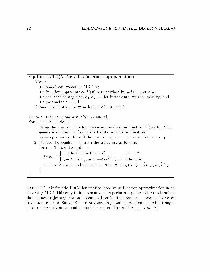
backgammon [Tesauro 92,Tesauro 94]. Tesauro modi�ed Sutton's TD(�) algorithm

x2.1 VALUE FUNCTION APPROXIMATION (VFA) 21
[Sutton 88], which is designed to approximate V � for a �xed policy �, to the task
of learning an optimal value function V � and optimal policy. The modi�cation is
simple: instead of generating sample trajectories by simulating a �xed policy �,
generate sample trajectories by simulating the policy � which is greedy with respect
to the current value function approximation ~V :
�(x) = argmaxa2A
�R(x; a) +
Xx02X
P (x0jx; a) ~V (x0)�
(2.5)
(Occasional non-greedy \exploration" moves are also usually performed [Thrun 92,
Singh et al. 98], but were found unnecessary in backgammon because of the domain's
inherent stochasticity [Tesauro 92].) The modi�ed algorithm has been termed opti-
mistic TD(�) [Bertsekas and Tsitsiklis 96], because little is known of its convergence
properties. An implementation is sketched in Table 2.1.2. When � = 0, the algorithm
strongly resembles Real-Time Dynamic Programming (RTDP) [Barto et al. 95], ex-
cept that RTDP assigns target values at each state by a \full backup" (averaging over
all possible outcomes, as in value iteration) rather than TD(0)'s \sample backups"
(learning from only the single observed outcome). Applying optimistic TD(�) with
a multi-layer perceptron function approximator, Tesauro's program learned an eval-
uation function which produced expert-level backgammon play. These results have
been replicated by myself [Boyan 92] and others.
Tesauro's combination of optimistic TD(�) and neural networks has been ap-
plied to other domains, including elevator control [Crites and Barto 96] and job-shop
scheduling [Zhang and Dietterich 95]. (I will discuss the scheduling application in
detail in Section 7.2.) Nevertheless, it is important to note that when function ap-
proximators are used, optimistic TD(�) provides no guarantees of optimality. The
following paragraphs summarize the current convergence results for value function
approximation. For both the prediction learning (approximating V �) and control
learning (approximating V �) tasks, the relevant questions are (1) do the available
algorithms converge, and (2) if so, how good are their resulting approximations?
We �rst consider the case of approximating the policy value function V � of a �xed
policy �. The TD(�) family of algorithms applies here. When � = 1, TD(�) reduces to
performing stochastic gradient descent to minimize the squared di�erence between the
approximated predictions ~V � and the observed simulation outcomes. Under standard
conditions, using any parametric function approximator, this will converge to a local
optimum of the squared-error function. For su�ciently small �, however, TD(�) may
diverge when nonlinear function approximators are used [Bertsekas and Tsitsiklis 96].
Only in the case where the function approximator is a linear architecture over state
features has TD(�) been proven to converge for arbitrary � [Tsitsiklis and Roy 96].
22 LEARNING FOR SEQUENTIAL DECISION MAKING
Optimistic TD(�) for value function approximation:Given:� a simulation model for MDP X;
� a function approximator ~V (x) parametrized by weight vector w;� a sequence of step sizes �1; �2; : : : for incremental weight updating; and� a parameter � 2 [0; 1].
Output: a weight vector w such that ~V (x) � V �(x).
Set w := 0 (or an arbitrary initial estimate):for n := 1; 2; : : : do: f
1. Using the greedy policy for the current evaluation function ~V (see Eq. 2.5),generate a trajectory from a start state in X to termination:x0 ! x1 � � � ! xT . Record the rewards r0; r1; : : : rT received at each step.
2. Update the weights of ~V from the trajectory as follows:for i := T downto 0, do: f
targi :=
(rT (the terminal reward) if i = T
ri + � � targi+1 + (1� �) � ~V (xi+1) otherwise.
Update ~V 's weights by delta rule: w := w + �n(targi � ~V (xi))rw~V (xi).
gg
Table 2.1. Optimistic TD(�) for undiscounted value function approximation in anabsorbing MDP. This easy-to-implement version performs updates after the termina-tion of each trajectory. For an incremental version that performs updates after eachtransition, refer to [Sutton 87]. In practice, trajectories are often generated using amixture of greedy moves and exploration moves [Thrun 92,Singh et al. 98].
x2.1 VALUE FUNCTION APPROXIMATION (VFA) 23
A useful error bound has also been shown in the linear case: the resulting �t is worse
than the best possible linear �t by a factor of at most (1 � �)=(1 � ), assuming a
discount factor of < 1 [Tsitsiklis and Roy 96]. This implies that TD(1) is guaranteed
to produce the best �t, but the bound quickly deteriorates as � decreases. The same
qualitative conclusion applies (though the formula for the bound is more complex)
for = 1 [Bertsekas and Tsitsiklis 96].
We now proceed to the harder problem of approximating the optimal value func-
tion V �. First, independent of how we construct it, is an approximate value function~V useful for deriving a decision-making policy? Singh and Yee [94] show that if ~V
di�ers from V � by at most � at any state, then the expected return of the greedy
policy for ~V will be worse than that of the optimal policy by a factor of at most
2 �=(1� ). A similar result holds in the undiscounted case, assuming all policies are
proper ( is then replaced by a contraction factor in a suitably weighted max norm).
This bound is not particularly comforting, since 1=(1 � ) will be large in practical
applications, but at least it guarantees that policies cannot be arbitrarily bad.
How should we construct V �? In general, algorithms based on value iteration's
one-step-backup operator, such as optimistic TD(�), use function approximator pre-
dictions to assign new training values for that same function approximator|a re-
cursive process that may propagate and enlarge approximation errors, leading to pa-
rameter divergence. I have demonstrated empirically that such divergence can indeed
happen when o�ine value iteration is combined with commonly used function approx-
imators, such as polynomial regression and neural networks [Boyan and Moore 95].
Small illustrative examples of divergence have also been demonstrated [Baird 95,Gor-
don 95]. Sutton has argued that certain of these instabilities may be prevented by
sampling states along simulated trajectories, as optimistic TD(�) does [Sutton 96];
but there are no convergence proofs of this as yet.
Parameter divergence in o�ine value iteration can provably be prevented by us-
ing function approximators belonging to the class of averagers, such as k-nearest-
neighbor [Gordon 95]. However, this class excludes practical function approximators
which extrapolate trends beyond their training data (e.g., global or local polyno-
mial regression, neural networks). Residual algorithms, which attempt to blend opti-
mistic TD(�) with a direct minimization of the residual approximation errors in the
Bellman equation, are guaranteed stable with arbitrary parametric function approx-
imators [Baird 95]; these methods are promising but as yet unproven on real-world
problems.
24 LEARNING FOR SEQUENTIAL DECISION MAKING
2.1.3 Working Backwards
Value iteration (VI) computes V � by repeatedly sweeping over the state space, ap-
plying Equation 2.4 as an assignment statement (this is called a \one-step backup")
at each state in parallel. Suppose the lookup table is initialized with all 0's. Then
after the ith sweep of VI, the table will store the maximum expected return of a path
of length i from each state. For so-called stochastic shortest path problems in which
every trajectory produced by the optimal policy inevitably terminates in an absorbing
state [Bertsekas and Tsitsiklis 96], this corresponds to the intuition that VI works by
propagating correct V � values backwards, by one step per iteration, from the terminal
states.
I have explored the e�ciency and robustness gains possible when VI is modi�ed
to take advantage of the working-backwards intuition. There are two main classes
of MDPs for which correct V � values can be assigned by working strictly backwards
from terminal states:
1. deterministic domains with no positive-reward cycles and with every state able
to reach at least one terminal state. This class includes shortest-path and
minimum \cost-to-go" problems [Bertsekas and Tsitsiklis 96].
2. (possibly stochastic) acyclic domains: domains where no trajectory can pass
through the same state twice. Many problems naturally have this property (e.g.,
board-�lling games like tic-tac-toe and Connect-Four, industrial scheduling as
described in Section 2.3.4 below, and any �nite-horizon problem for which time
is a component of the state).
Using VI to solve MDPs belonging to either of these special classes can be quite
ine�cient, since VI performs backups over the entire space, whereas the only back-
ups useful for improving V � are those on the \frontier" between already-correct and
not-yet-correct V � values. In fact, for small problems there are classical algorithms
for both problem classes which compute V � more e�ciently by explicitly working
backwards: for the deterministic class, Dijkstra's shortest-path algorithm; and for the
acyclic class, Directed-Acyclic-Graph-Shortest-Paths (DAG-SP) [Cormen et
al. 90].1 DAG-SP �rst topologically sorts the MDP, producing a linear ordering of
the states in which every state x precedes all states reachable from x. Then, it runs
through that list in reverse, performing one backup per state. Worst-case bounds for
VI, Dijkstra, and DAG-SP in deterministic domains with X states and A actions per
state are O(AX2), O(AX logX), and O(AX), respectively.
1Although Cormen et al. [90] present DAG-SP only for deterministic acyclic problems, it appliesstraightforwardly to the stochastic case.

x2.2 VFA IN DETERMINISTIC DOMAINS: \GROW-SUPPORT" 25
Another di�erence between VI and working backwards is that VI repeatedly re-
estimates the values at every state, using old predictions to generate new training
values. By contrast, Dijkstra and DAG-SP are always explicitly aware of which states
have their V � values already known, and can hold those values �xed. This distinction
is important in the context of generalization and the possibility of approximation
error.
In sum, I have presented two reasons why working strictly backwards may be
desirable: e�ciency, because updates need only be done on the \frontier" rather
than all over state space; and robustness, because correct V � values, once assigned,
need never again be changed. I have therefore investigated generalizations of the
Dijkstra and DAG-SP algorithms speci�cally modi�ed to accommodate huge state
spaces and value function approximation. My variant of Dijkstra's algorithm, called
Grow-Support, was presented in [Boyan and Moore 95] and is summarized brie y
in Section 2.2. My variant of DAG-SP is an algorithm called ROUT [Boyan and
Moore 96], which I describe in more detail and with new results in Section 2.3. Other
researchers have also investigated learning control by working backwards, notably
Atkeson [94] for the case of deterministic domains with continuous dynamics.
2.2 VFA in Deterministic Domains: \Grow-Support"
This section summarizes Grow-Support, an algorithm for value function approxima-
tion in large, deterministic, minimum-cost-to-goal domains [Boyan and Moore 95].
Grow-Support is designed to construct the optimal value function with a generalizing
function approximator while remaining robust and stable. It recognizes that function
approximators cannot always be relied upon to �t the intermediate value functions
produced by value iteration. Instead, it assumes only that the function approximator
can represent the �nal V � function accurately, if given accurate training values for a
prespeci�ed collection of sample states. The speci�c principles of Grow-Support are
as follows:
1. We maintain a \support" subset of sample states whose �nal V � values have
been computed, starting with terminal states and then growing backward from
there. The �tter ~V is trained only on these values, which we assume it is capable
of �tting.
2. Instead of propagating values by one-step backups, we use rollouts|simulated
trajectories guided by the current greedy policy on ~V . They explicitly verify the
achievability of a state's estimated future reward before that state is added to
the support set. In a rollout, the new ~V training value is derived from rewards
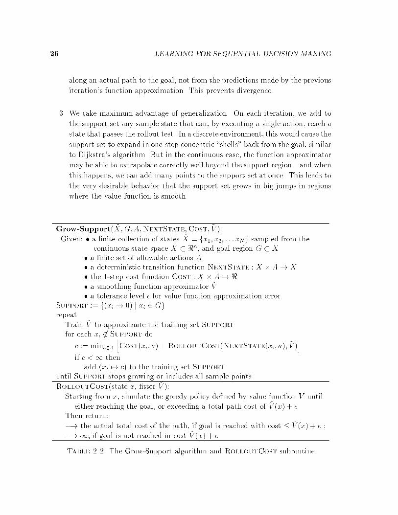
26 LEARNING FOR SEQUENTIAL DECISION MAKING
along an actual path to the goal, not from the predictions made by the previous
iteration's function approximation. This prevents divergence.
3. We take maximum advantage of generalization. On each iteration, we add to
the support set any sample state that can, by executing a single action, reach a
state that passes the rollout test. In a discrete environment, this would cause the
support set to expand in one-step concentric \shells" back from the goal, similar
to Dijkstra's algorithm. But in the continuous case, the function approximator
may be able to extrapolate correctly well beyond the support region|and when
this happens, we can add many points to the support set at once. This leads to
the very desirable behavior that the support set grows in big jumps in regions
where the value function is smooth.
Grow-Support(X̂;G;A;NextState;Cost; ~V ):
Given: � a �nite collection of states X̂ = fx1; x2; : : : xNg sampled from thecontinuous state space X � <n, and goal region G � X
� a �nite set of allowable actions A� a deterministic transition function NextState : X �A! X� the 1-step cost function Cost : X �A! <� a smoothing function approximator ~V� a tolerance level � for value function approximation error
Support := f(xi 7! 0) j xi 2 Ggrepeat
Train ~V to approximate the training set Supportfor each xi 62 Support do
c := mina2AhCost(xi; a) +RolloutCost(NextState(xi; a); ~V )
iif c <1 then
add (xi 7! c) to the training set Supportuntil Support stops growing or includes all sample points.
RolloutCost(state x, �tter ~V ):
Starting from x, simulate the greedy policy de�ned by value function ~V until
either reaching the goal, or exceeding a total path cost of ~V (x) + �.Then return:
�! the actual total cost of the path, if goal is reached with cost � ~V (x) + � ;
�!1, if goal is not reached in cost ~V (x) + �.
Table 2.2. The Grow-Support algorithm and RolloutCost subroutine

x2.3 VFA IN ACYCLIC DOMAINS: \ROUT" 27
The algorithm is sketched in Table 2.2. In a series of experiments reported in
[Boyan and Moore 95], I found that Grow-Support is more robust than value iteration
with function approximation. (Several follow-up studies provide additional insight
into value iteration's potential for divergence [Gordon 95,Sutton 96].) Grow-Support
was also seen to be no more computationally expensive, and often much cheaper,
despite the overhead of performing rollouts. Reasons for this include: (1) the rollout
test is not expensive; (2) once a state has been added to the support, its value is
�xed and it needs no more computation; and most importantly, (3) the aggressive
exploitation of generalization enables the algorithm to converge in very few iterations.
It is easy to prove that Grow-Support will always terminate after a �nite number
of iterations. If the function approximator is inadequate for representing the V �
function, Grow-Support may terminate before adding all sample states to the support
set. When this happens, we then know exactly which of the sample states are having
trouble and which have been learned. This suggests potential schemes for adaptively
adding sample states in problematic regions. The ROUT algorithm, described next,
does adaptively generate its own set of sample states for learning.
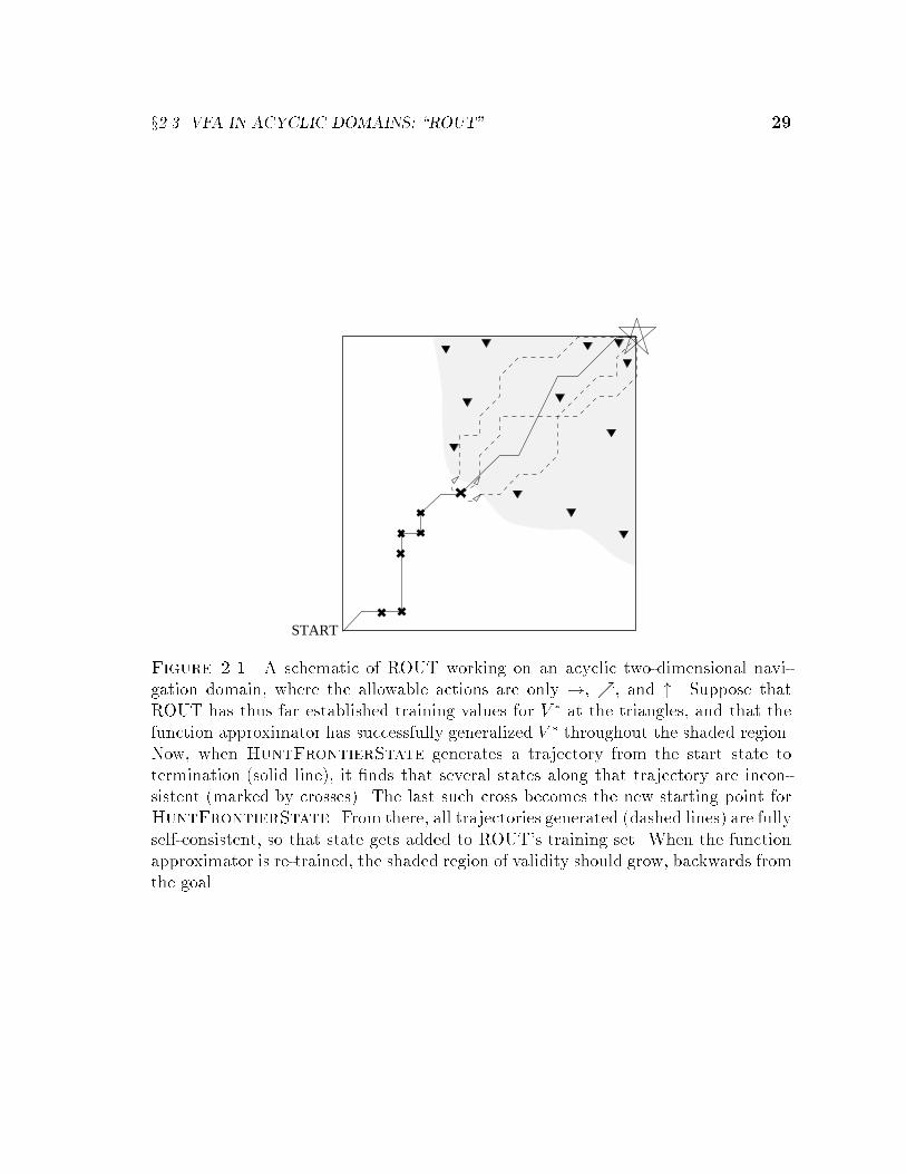
2.3 VFA in Acyclic Domains: \ROUT"
As Grow-Support scaled up Dijkstra's algorithm for deterministic domains, ROUT
aims to scale up DAG-Shortest-Paths (DAG-SP) for stochastic, acyclic domains. In
large combinatorial spaces requiring function approximation, DAG-SP's key prepro-
cessing step|topologically sorting the entire state space|is no longer tractable. In-
stead, ROUT must expend some extra e�ort to identify states on the current frontier.
Once identi�ed (as described below), a frontier state is assigned its optimal V � value
by a simple one-step backup, and this fstate!valueg pair is added to a training set
for a function approximator. I determine the training value by a one-step backup
rather than rollouts because, unlike the deterministic MDPs to which Grow-Support
applies, stochastic MDPs would require performing not one but many rollouts for
accurate value determination. However, ROUT still does use an analogue of Grow-
Support's \rollout test" to identify the states at which the one-step backup may be
safely applied.
In sum, ROUT's main loop consists of identifying a frontier state; determining its
V � value; and retraining the approximator. The training set, constructed adaptively,
grows backwards from the goal. HuntFrontierState is the key subroutine ROUT
uses to identify a good state to add to the training set. The criteria for such a state
x are as follows:

28 LEARNING FOR SEQUENTIAL DECISION MAKING
1. All states reachable from x should already have their V � values correctly ap-
proximated by the function approximator. This ensures that the policy from x
onward is optimal, and that a correct target value for V �(x) can be assigned.
2. x itself should not already have its V � value correctly approximated. This
condition aims to keep the training set as small as possible, by excluding states
whose values are correct anyway thanks to good generalization.
3. x should be a state that we care to learn about. For that reason, ROUT
considers only states which occur on trajectories emanating from a starting
state of the MDP.
The HuntFrontierState operation returns a state which with high probability
satis�es these properties. It begins with some state x and generates a number of
trajectories from x, each time checking to see whether all states along the trajectory
are self-consistent (i.e., satisfy Equation 2.4 to some tolerance �). If all states after
x on all sample trajectories are self-consistent, then x is deemed ready, and ROUT
will add x to its training set. If, on the other hand, a trajectory from x reveals any
inconsistencies in the approximated value function, then we ag that trajectory's last
such inconsistent state, and restart HuntFrontierState from there. Table 2.3
speci�es the algorithm, and Figure 2.3 illustrates how the routine works.
The parameters of the ROUT algorithm are H, the number of trajectories gen-
erated to certify a state's readiness, and �, the tolerated Bellman residual. ROUT's
convergence to the optimal V �, assuming the function approximator can �t the V �
training set perfectly, can be guaranteed in the limiting case where H !1 (assuring
exploration of all states reachable from x) and � = 0. In practice, of course, we want
to be tolerant of some approximation error. Typical settings I used were H = 20 and
� = roughly 5% of the range of V �.
The following sections present experimental results with ROUT on three domains:
a prediction task, a two-player dice game, and a k-armed bandit problem. For all
problems, I compare ROUT's performance with that of optimistic TD(�) given the
equivalent function approximator. I measure the time to reach best performance
(in terms of total number of state evaluations performed) and the quality of the
learned value function (in terms of Bellman residual, closeness to the true V �, and
performance of the greedy control policy). The results show that ROUT learned
evaluation functions which were as good or better than those learned by TD(�), and
used an order of magnitude less training data in doing so. I also report preliminary
results on a fourth domain, a simpli�ed production scheduling task.
x2.3 VFA IN ACYCLIC DOMAINS: \ROUT" 29
START
Figure 2.1. A schematic of ROUT working on an acyclic two-dimensional navi-gation domain, where the allowable actions are only !, %, and ". Suppose thatROUT has thus far established training values for V � at the triangles, and that thefunction approximator has successfully generalized V � throughout the shaded region.Now, when HuntFrontierState generates a trajectory from the start state totermination (solid line), it �nds that several states along that trajectory are incon-sistent (marked by crosses). The last such cross becomes the new starting point forHuntFrontierState. From there, all trajectories generated (dashed lines) are fullyself-consistent, so that state gets added to ROUT's training set. When the functionapproximator is re-trained, the shaded region of validity should grow, backwards fromthe goal.

30 LEARNING FOR SEQUENTIAL DECISION MAKING
ROUT(start states X̂, �tter ~V ):/* Assumes that the world model MDP is known and acyclic. */
initialize training set S := ;, and ~V := an arbitrary �t;repeat:
for each start state x 2 X̂ not yet marked \done", do:
s := HuntFrontierState(x; ~V );
add fs 7! one-step-backup(s)g to training set S and re-train �tter ~V on S;if (s = x), then mark start state x as \done".
until all start states in X̂ are marked \done".
HuntFrontierState(state x, �tter ~V ):/* If the value function is self-consistent on all trajectories from x, return
x. (That is determined probabilistically by Monte Carlo trials.) Other-wise, return a state on a trajectory from x for which the self-consistencyproperty is true. */
for each legal action a 2 A(x), do:repeat up to H times:
generate a trajectory ~T from x to termination, starting with action a;
let y be the last state on ~T with Bellman residual > �;if (y 6= ;) and (y 6= x), then break out of loops, and
restart procedure with HuntFrontierState(y; ~V )./* reaching this point, x's subtree is deemed all self-consistent and correct! */return x.
Table 2.3. The ROUT algorithm and the HuntFrontierState subroutine

x2.3 VFA IN ACYCLIC DOMAINS: \ROUT" 31
2.3.1 Task 1: Stochastic Path Length Prediction
The \Hopworld" is a small domain designed to illustrate how ROUT combines working
backwards, adaptive sampling and function approximation. The domain is an acyclic
Markov chain of 13 states in which each state has two equally probable successors:
one step to the right or two steps to the right. The transition rewards are such
that for each state V �(n) = �2n. Our function approximator ~V makes predictions
by interpolating between values at every fourth state. This is equivalent to using a
linear approximator over the four-element feature vector representation depicted in
Figure 2.2.
-3.0 -3.0
-3.0 -3.0
START
[0, 0, 1/4, 3/4]
[0, 0, 1/2, 1/2] [0, 0, 0, 1]
[0, 0, 3/4, 1/4]
[1, 0, 0, 0]
[3/4, 1/4, 0, 0]
[1/2, 1/2, 0, 0]
12 11 10 3 2 1 0-2.0
-3.0
-3.0
-3.0
-3.0
Figure 2.2. The Hopworld Markov chain. Each state is represented by a four-element feature vector as shown. The function approximator is linear.
In ROUT, we �t the training set using a batch least-squares �t. In TD, the coef-
�cients are updated using the delta rule with a hand-tuned learning rate. The results
are shown in Table 2.4. ROUT's performance is e�cient and predictable on this
contrived problem. At the start, HuntFrontierState �nds ~V is inconsistent and
trains ~V (1) and ~V (2) to be -2 and -4, respectively. Linear extrapolation then forces
states 3 and 4 to be correct. On the third iteration, ~V (5) is spotted as inconsistent
and added to the training set, and bene�cial extrapolation continues. By compari-
son, TD also has no trouble learning V �, but requires many more evaluations. This is
because TD trains blindly on all transitions, not only the useful ones; and because its
updates must be done with a fairly small learning rate, since the domain is stochastic.
TD could be improved by an adaptive learning rate, or better yet, by eliminating its
learning rates and performing Least-Squares TD as described later in Section 6.1.2.
2.3.2 Task 2: A Two-Player Dice Game
\Pig" is a two-player children's dice game. Each player starts with a total score of
zero, which is increased on each turn by dice rolling. The �rst to 100 wins. On her
turn, a player accumulates a subtotal by repeatedly rolling a 6-sided die. If at any
time she rolls a 1, however, she loses the subtotal and gets only 1 added to her total.

32 LEARNING FOR SEQUENTIAL DECISION MAKING
Thus, before each roll, she must decide whether to (a) add her currently accumulated
subtotal to her permanent total and pass the turn to the other player; or (b) continue
rolling, risking an unlucky 1.
Pig belongs to the class of symmetric, alternating Markov games. This means
that the minimax-optimal value function can be formulated as the unique solution
to a system of generalized Bellman equations [Littman and Szepesv�ari 96] similar to
Equation 2.4. The state space, with two-player symmetry factored out, has 515,000
positions|large enough to be interesting, but small enough that computing the exact
V � is tractable.
For input to the function approximator, we represent states by their natural 3-
dimensional feature representation: X's total, O's total, and X's current subtotal.
The approximator is a standard MLP with two hidden units. In ROUT, the network
is retrained to convergence (at most 1000 epochs) each time the training set is aug-
mented. Note that this extra cost of ROUT is not re ected in the results table, but
for practical applications, a far faster approximator than backpropagation would be
used with ROUT.2
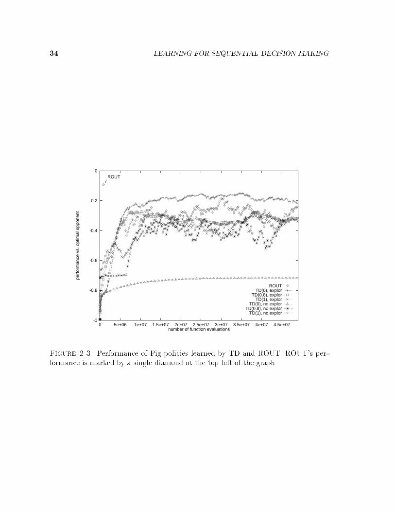
The Pig results are charted in Table 2.4 and graphed in Figure 2.3. The graph
shows the learning curves for the best single trial of each of six classes of runs: TD(0),
TD(0.8) and TD(1), with and without exploration. (The vertical axis measures per-
formance in expected points per game against the minimax optimal player, where
+1 point is awarded for a win and �1 for a loss.) The best TD run, TD(0) with
exploration, required about 30 million evaluations to reach its best performance of
about �0:15. By contrast, ROUT completed successfully in under 1 million evalua-
tions, and performed at the signi�cantly higher level of �0:09. ROUT's adaptively
generated training set contained only 133 states.
2.3.3 Task 3: Multi-armed Bandit Problem
Our third test problem is to compute the optimal policy for a �nite-horizon k-armed
bandit [Berry and Fristedt 85]. While an optimal solution in the in�nite-horizon
case can be found e�ciently using Gittins indices, solving the �nite-horizon problem
is equivalent to solving a large acyclic, stochastic MDP in belief space [Berry and
Fristedt 85]. I show results for k = 3 arms and a horizon of n = 25 pulls, where
the resulting MDP has 736,281 states. Solving this MDP by DAG-SP produces the
2Unlike TD, which works only with parametric function approximators for which rw~V (x) can be
calculated, ROUT can work with arbitrary function approximators, including batch methods suchas projection-pursuit and locally weighted regression. For these comparative experiments, however,we used linear or neural network �ts for both algorithms.
x2.3 VFA IN ACYCLIC DOMAINS: \ROUT" 33
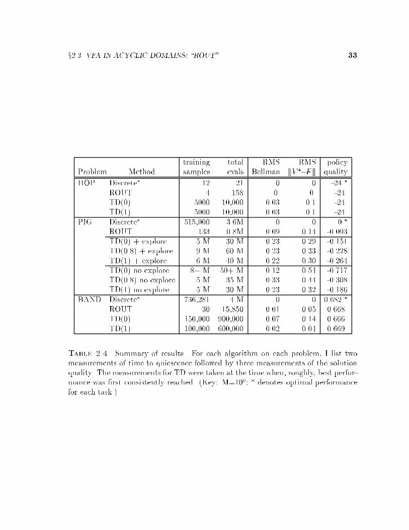
training total RMS RMS policyProblem Method samples evals Bellman kV ��Fk quality
HOP Discrete� 12 21 0 0 -24 �
ROUT 4 158 0. 0. -24TD(0) 5000 10,000 0.03 0.1 -24TD(1) 5000 10,000 0.03 0.1 -24
PIG Discrete� 515,000 3.6M 0 0 0 �
ROUT 133 0.8M 0.09 0.14 -0.093TD(0) + explore 5 M 30 M 0.23 0.29 -0.151TD(0.8) + explore 9 M 60 M 0.23 0.33 -0.228TD(1) + explore 6 M 40 M 0.22 0.30 -0.264TD(0) no explore 8+ M 50+ M 0.12 0.54 -0.717TD(0.8) no explore 5 M 35 M 0.33 0.44 -0.308TD(1) no explore 5 M 30 M 0.23 0.32 -0.186
BAND Discrete� 736,281 4 M 0 0 0.682 �
ROUT 30 15,850 0.01 0.05 0.668TD(0) 150,000 900,000 0.07 0.14 0.666TD(1) 100,000 600,000 0.02 0.04 0.669
Table 2.4. Summary of results. For each algorithm on each problem, I list twomeasurements of time to quiescence followed by three measurements of the solutionquality. The measurements for TD were taken at the time when, roughly, best perfor-mance was �rst consistently reached. (Key: M=106; * denotes optimal performancefor each task.)
34 LEARNING FOR SEQUENTIAL DECISION MAKING
-1
-0.8
-0.6
-0.4
-0.2
0
0 5e+06 1e+07 1.5e+07 2e+07 2.5e+07 3e+07 3.5e+07 4e+07 4.5e+07
perf
orm
ance
vs.
opt
imal
opp
onen
t
number of function evaluations
ROUT/
ROUTTD(0), explor
TD(0.8), explorTD(1), explor
TD(0), no explorTD(0.8), no explor
TD(1), no explor
Figure 2.3. Performance of Pig policies learned by TD and ROUT. ROUT's per-formance is marked by a single diamond at the top left of the graph.

x2.3 VFA IN ACYCLIC DOMAINS: \ROUT" 35
optimal exploration policy, which has an expected reward of 0.6821 per pull.
Each state is encoded as a six-dimensional feature vector of [#succarm1; #failarm1;
#succarm2; #failarm2; #succarm3; #failarm3] and attempted to learn a neural network
approximation to V � with TD(0), TD(1), and ROUT. Again, the parameters for all
algorithms were tuned by hand.
The results are shown in Table 2.4. All methods do spectacularly well, although
the TD methods again require more trajectories and more evaluations. Careful in-
spection of the problem reveals that a globally linear value function, extrapolated
from the states close to the end, has low Bellman residual and performs very nearly
optimally. Both ROUT and TD successfully exploit this linearity.
2.3.4 Task 4: Scheduling a Factory Production Line
Production scheduling, the problem of deciding how to con�gure a factory sequentially
to meet demands, is a critical problem throughout the manufacturing industry.3 We
assume we have a modest number of products (2{100) and must produce enough
of each to keep warehouse stocks high enough to satisfy customer requests for bulk
shipments. This production model is common, for example, for most goods found in
a supermarket.
An instance of the production scheduling problem is composed of �ve parts:
Machines and products. This is a list of what machines are present in the factory,
and what products can be made on the machines. There may be complex
constraints such as \machine A can only make product 1 when machine B is
not making product 3." A complete, legal assignment of products onto the set of
machines is called a con�guration. There is also a special \closed" con�guration
which represents a decision to shut the factory down.
Changeover times. It generally takes a certain amount of time to switch the factory
from one con�guration to another. During that time, there is no production.
The problem de�nition includes a (possibly stochastic) estimate of how long it
takes to change each con�guration to each other con�guration.
Production rates. Each con�guration produces a set of products at a certain rate.
There may be dependencies between the machines. For example, machine B
may produce product 2 faster if machine A is also producing product 2. The
actual production rates in the factory may be very stochastic; for example, some
machines may jam frequently, causing irregular delays on the production line.
3The application of RL to production scheduling reported here is the result of a collaborationwith Je� Schneider and Andrew Moore [Schneider et al. 98].
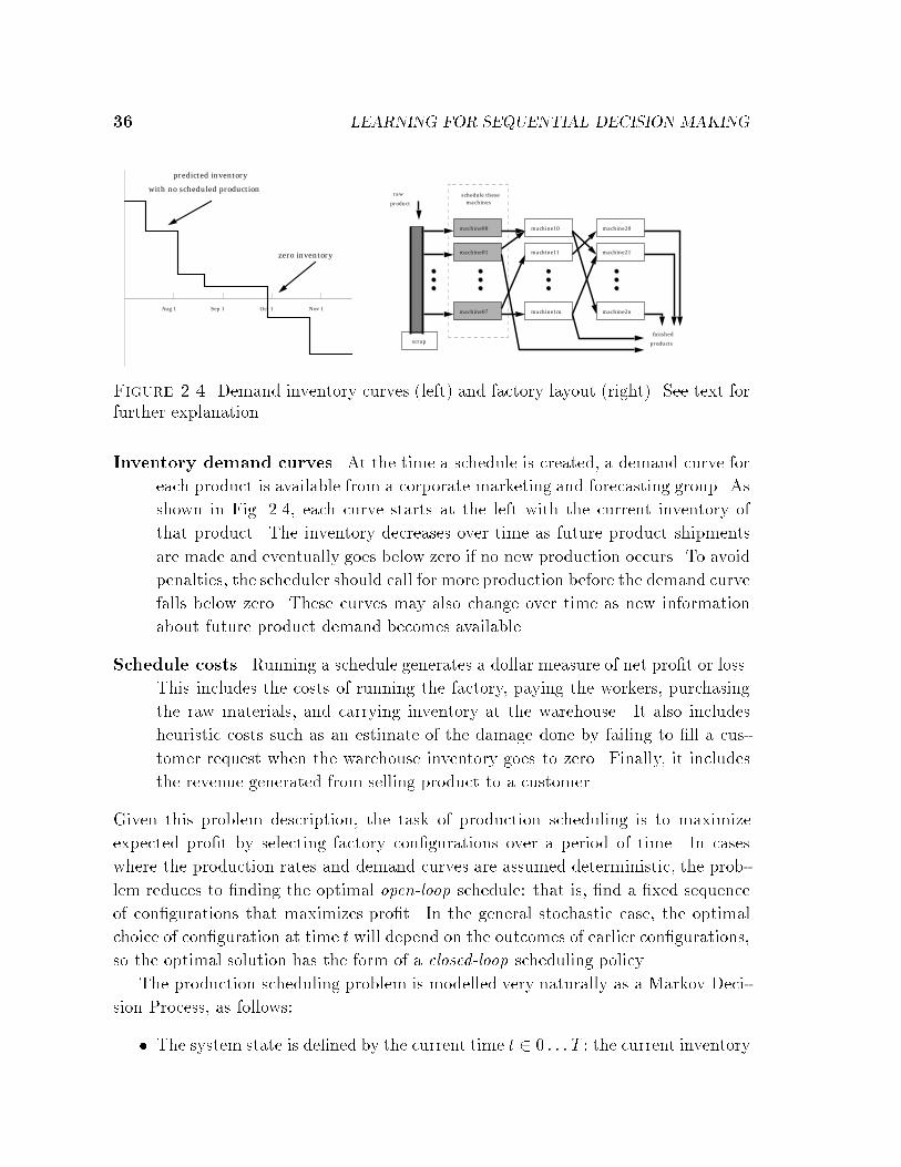
36 LEARNING FOR SEQUENTIAL DECISION MAKING
Aug 1 Sep 1 Oct 1 Nov 1
predicted inventory
with no scheduled production
zero inventory
machine07
machine00
machine01
machine1m
machine11
machine10
machine2n
machine21
machine20
scrap
raw
product
finished
products
schedule thesemachines
Figure 2.4. Demand inventory curves (left) and factory layout (right). See text forfurther explanation.
Inventory demand curves. At the time a schedule is created, a demand curve for
each product is available from a corporate marketing and forecasting group. As
shown in Fig. 2.4, each curve starts at the left with the current inventory of
that product. The inventory decreases over time as future product shipments
are made and eventually goes below zero if no new production occurs. To avoid
penalties, the scheduler should call for more production before the demand curve
falls below zero. These curves may also change over time as new information
about future product demand becomes available.
Schedule costs. Running a schedule generates a dollar measure of net pro�t or loss.
This includes the costs of running the factory, paying the workers, purchasing
the raw materials, and carrying inventory at the warehouse. It also includes
heuristic costs such as an estimate of the damage done by failing to �ll a cus-
tomer request when the warehouse inventory goes to zero. Finally, it includes
the revenue generated from selling product to a customer.
Given this problem description, the task of production scheduling is to maximize
expected pro�t by selecting factory con�gurations over a period of time. In cases
where the production rates and demand curves are assumed deterministic, the prob-
lem reduces to �nding the optimal open-loop schedule: that is, �nd a �xed sequence
of con�gurations that maximizes pro�t. In the general stochastic case, the optimal
choice of con�guration at time t will depend on the outcomes of earlier con�gurations,
so the optimal solution has the form of a closed-loop scheduling policy.
The production scheduling problem is modelled very naturally as a Markov Deci-
sion Process, as follows:
� The system state is de�ned by the current time t 2 0 : : : T ; the current inventory
x2.3 VFA IN ACYCLIC DOMAINS: \ROUT" 37
of each product p1 : : : pN ; and, if there are con�guration-dependent changeover
times, the current factory con�guration.
� The action set consists of all legal factory con�gurations. We assume a discrete-
time model, so the con�guration chosen at time t will run unchanged until time
t+ 1.
� The stochastic transition function applies a simulation of the factory to com-
pute the change in all inventory levels realized by running con�guration ct for 1
timestep. This model handles random variations in production rates straight-
forwardly; it also handles changeover times by simply decreasing production in
proportion to the (possibly stochastic) downtime. The time t is incremented on
each step, and the process terminates when t = T .
� The immediate reward function is computed from the inventory levels, based
on the demand curve at time t. It incorporates the revenues from production,
penalties from late production, employee costs, operating costs and changeover
cost incurred during the period. On the �nal time period (transition from
t = T � 1 to T ), a terminal \reward" assigns additional penalties for any
outstanding unsatis�ed demands.
The MDP model fully represents uncertainty in production rates and changeover
times. As de�ned here, the model also handles noise in the demands if that noise
is time-independent, but it cannot account for the possibility of the demand curves
being randomly updated in the middle of a schedule, since that would make the MDP
transition probabilities nonstationary. Finally, since the current time t is included as
part of the state, the MDP is acyclic: ROUT may be applied.
I applied ROUT to a highly simpli�ed version of a real factory's scheduling prob-
lem. The task involves scheduling 8 weeks of production; however, con�gurations may
be changed only at 2-week intervals, and only 17 con�guration choices are available.
Of these 17, nine have deterministic production rates; the other eight each have two
stochastic outcomes, producing only 1=3 of their usual amount with probability 0:5.
With a total of 9 � 1 + 8 � 2 = 25 outcomes possible from every state, and four
scheduling periods, there are 254 = 390; 625 possible trajectories through the space.
The optimal policy can be computed by tabulating V �(x) at every possible interme-
diate state x of the factory, of which there are 1 + 25 + 252 + 253 = 16; 276. The
optimal policy results in an expected cumulative reward of �$22:8M. By contrast, a
random schedule attains a reward of �923M . A greedy policy, which at each step
selects a con�guration to maximize only the next period's pro�t, attains �$97:9M.

38 LEARNING FOR SEQUENTIAL DECISION MAKING
I applied ROUT to this instance, trying two di�erent memory-based function
approximators: 1-nearest neighbor and locally weighted linear regression [Cleveland
and Devlin 88]. (The local regression used a kernel width of 18of the range of each
input dimension in the training data; this fraction was tuned manually over powers of12 .) Since these function approximators are nonparametric, TD(�) cannot be used to
train them, so ROUT is compared only to the optimal, greedy, and random policies.
ROUT's exploration and tolerance parameters were also tuned manually.
Algorithm Mean Pro�t 95% C.I. optimal runsOptimal -22.8 1Random -923.2 �58.7 0Greedy -97.9 �15.1 0ROUT + nearest neighbor N/A 0ROUT + locally weighted linear -45.0 �16.9 10/16
Table 2.5. Results on the production scheduling task
Table 2.5 summarizes the results. When nearest-neighbor was used as the function
approximator, ROUT did not obtain su�cient generalization from its training set and
failed to terminate within a limit of several hours. However, with a locally weighted
regression model, ROUT did run to completion and produced an approximate value
function which signi�cantly outperformed the greedy policy. Moreover, over half of
these runs did indeed terminate with the optimal closed-loop scheduling policy. In
these cases, ROUT's �nal self-built training set for value function approximation
consisted of only about 110 training points|a substantial reduction over the 16; 276
required for full tabulation of V �. ROUT's total running time (� 1 hour on a 200 MHz
Pentium Pro) was roughly half of that required to enumerate V � manually.
From these preliminary results, I conclude that ROUT does indeed have the po-
tential to approximate V � extremely well, given a suitable function approximator
for the domain. However, since it runs quite slowly on even this simple problem,
I believe ROUT will not scale up to practical scheduling instances without further
modi�cation.
2.4 Discussion
When a function approximator is capable of �tting V �, ROUT will, in the limit, �nd
it. However, for ROUT to be e�cient, the frontier must grow backward from the goal
quickly, and this depends on good extrapolation from the training set. When good
extrapolation does not occur, ROUT may become stuck, repeatedly adding points

x2.4 DISCUSSION 39
near the goal region and never progressing backwards. Some function approximators
may be especially well-suited to ROUT's required extrapolation from accurate train-
ing data, and this deserves further exploration. Another promising re�nement would
be to adapt the tolerance level �, thereby guaranteeing progress at the expense of
accuracy.
Grow-Support and ROUT represent �rst steps toward a new class of algorithms
for solving large-scale MDPs. Their primary innovation is that, without falling prey
to the curse of dimensionality, they are able to explicitly represent which states are
already solved and which are not yet solved. Using this information, they \work
backwards," computing accurate V � values at targeted unsolved states using either
function approximator predictions at solved states or Monte Carlo rollouts. Impor-
tantly, and unlike the Dijkstra and DAG-SP exact algorithms on which they are
based, they grow the solution set for V � back from the goal without requiring an
explicit backward model for the MDP. Only forward simulations are used; this con-
strains the distribution of visited states to areas that are actually reachable during
task execution. By treating solved and unsolved states di�erently, Grow-Support and
ROUT eliminate the possibility of divergence caused by repeated value re-estimation.
This chapter has reviewed the state of the art in reinforcement learning, a �eld
which is grounded solidly in the theory of dynamic programming but provides few
guarantees for the practical cases where function approximators, rather than lookup
tables, must be used to construct the value function. I have described two novel
algorithms for approximating V � which are guaranteed stable and which perform
well in practice. In the remaining chapters of this thesis, I consider the simpler VFA
problem of approximating V � for a �xed policy �, on which TD(�) with linear function
approximators does come with strong convergence guarantees|and I demonstrate a
practical way of exploiting these approximations to improve search performance on
global optimization tasks.

40
41
Chapter 3
Learning Evaluation Functions for
Global Optimization
3.1 Introduction
3.1.1 Global Optimization
Global optimization|the problem of �nding the best possible con�guration from a
large space of possible con�gurations|is among the most fundamental of computa-
tional tasks. Its numerous applications in science, engineering, and industry include
� design and layout: optimizing VLSI circuit designs for computer architectures
[Wong et al. 88], packing automobile components under a car hood [Szykman
and Cagan 95], architectural design, magazine page layout
� resource allocation: airline scheduling [Subramanian et al. 94], school timetabling,
factory production scheduling, military logistics planning
� parameter optimization: generating accurate models for weather prediction,
ecosystem modeling [Duan et al. 92], economic modeling, tra�c simulations,
intelligent database querying [Boyan et al. 96]
� scienti�c analysis: computational biology (gene sequencing) [Karp 97], compu-
tational chemistry (protein folding) [Neumaier 97]
� engineering: medical robotics (radiotherapy for tumor treatment) [Webb 91],
computer vision (line matching) [Beveridge et al. 96]
Formally, an instance of global optimization consists of a state space X and an
objective function Obj : X ! <. The goal is to �nd a state x� 2 X which minimizes
Obj, that is, Obj(x�) � Obj(x) 8x 2 X. If the space X is so small that every state
can be evaluated, then obtaining the exact solution x� is trivial; otherwise, special
knowledge of the problem structure must be exploited. For example, if X is a convex
linearly constrained subset of <n and Obj is linear, then x� can be found e�ciently
by linear programming.

42 LEARNING FOR GLOBAL OPTIMIZATION
But for many important optimization problems, e�cient solution methods are
unknown. Practical combinatorial optimization problems where X is �nite but enor-
mous, such as the applications listed under \design and layout" and \resource alloca-
tion" above, all too often fall into the class of NP-hard problems, for which e�cient
exact algorithms are thought not to exist [Garey and Johnson 79]. Recent progress
in cutting-plane and branch-and-bound algorithms, especially as applied to mixed-
integer linear programming and Travelling Salesperson Problems, has led to exact
solutions for some large NP-hard problem instances [Applegate et al. 95, Subrama-
nian et al. 94]. However, for most real-world domains, practitioners resort to heuristic
approximation methods which seek good approximate solutions.
To illustrate the discussion that follows, I will present an example optimization
instance from the domain of one-dimensional bin-packing. In bin-packing, we are
given a bin capacity C and a list L = (a1; a2; :::an) of n items, each having a size
s(ai) > 0. The goal is to pack the items into as few bins as possible, i.e., partition
them into a minimum number m of subsets B1; B2; :::; Bm such that for each Bj ,Pai2Bj
s(ai) � C. This problem has many real-world applications, including loading
trucks subject to weight limitations, packing commercials into station breaks, and
cutting stock materials from standard lengths of cable or lumber [Co�man et al. 96].
It is also a classical NP-complete optimization problem [Garey and Johnson 79].
Figure 3.1 depicts a small bin-packing instance with thirty items. Packed optimally,
these items �ll 9 bins exactly to capacity.
29 28 27 26 25 24 23 22 21 20 19 18 17 16 15 14 13 12 11 10 9 8 7 6 5 4 3 2 1 0
8 7 6 5 4 3 2 1 0
Figure 3.1. A small bin-packing domain. Left: initial state (30 items, each in itsown bin). Right: the global optimum (nine bins packed with 0 waste).
x3.1 INTRODUCTION 43
3.1.2 Local Search
Many special-purpose approximation algorithms have been proposed and analyzed
for the bin-packing problem [Co�man et al. 96]. However, we will focus instead on
a broad class of general-purpose algorithms for the general global optimization prob-
lem: the class of local search algorithms. All of these work by de�ning a neighborhood
N(xi) � X for each state xi 2 X. Usually, the neighborhood of x consists of simple
perturbations to x|states whose new Obj value can be computed incrementally and
e�ciently from Obj(x). However, complex neighborhood structures can also be e�ec-
tive (e.g., the Lin-Kernighan algorithm for the Traveling Salesman Problem [Lin and
Kernighan 73]). The neighborhood structure and objective function together give
rise to a cost surface over the state space. Local search methods start at some initial
state, perhaps chosen randomly, and then search for a good solution by iteratively
moving over the cost surface from state to neighboring state.
The simplest local search method is known variously as greedy descent, iterative
improvement or, most commonly, hillclimbing.1 Hillclimbing's essential property is
that it never accepts a move that worsens Obj. There are several variants. In steepest-
descent hillclimbing, every neighbor x0 2 N(x) is evaluated, and the neighbor with
minimal Obj(x0) is chosen as the successor state (ties are broken randomly). Steepest-
descent terminates as soon as it encounters a local optimum, a state x for which
Obj(x) � Obj(x0) 8x0 2 N(x). In another variant, stochastic hillclimbing (also known
as �rst-improvement), random neighbors of x are evaluated one by one, and the �rst
one which improves on Obj(x) is chosen. Whether or not to accept equi-cost moves, to
a neighboring state of equal cost, is a parameter of the algorithm. Another parameter,
called patience, governs termination: the search halts after patience neighbors have
been evaluated consecutively and all found unhelpful. Thus, the �nal state reached
is only probabalistically, not with certainty, a local optimum. Despite this, stochastic
hillclimbing is often preferred for its ability to �nd a good solution very quickly.
Hillclimbing's obvious weakness is that it gets stuck at the �rst local optimum
it encounters. Alternative local search methods provide a variety of heuristics for
accepting some moves to worse neighbors. The possibilities include
� \Force-best-move" approaches: move to the best neighbor, even if its value is
worse. (This approach has been successful in the GSAT algorithm [Selman and
Kautz 93].)
1In this dissertation, I will use the term \hillclimbing" even though we seek a minimum of thecost surface. Simply imagine that the goal of our metaphorical mountain climber is to minimize hisdistance from the sky.

44 LEARNING FOR GLOBAL OPTIMIZATION
� More generally, \biased random walk" approaches: allow moves to worse neigh-
bors stochastically, perhaps depending on how much worse the neighbor is.
(This approach has been successful in the WALKSAT algorithm [Selman et
al. 96] and others.)
� Simulated annealing [Kirkpatrick et al. 83]. This popular approach is like the
biased random walk, but gradually lowers the probability of accepting a move
to a worse neighbor. Search terminates at a local optimum after the proba-
bility falls to zero. Simulated annealing approaches are discussed in detail in
Appendix B.
� Multiple restarting. Because stochastic hillclimbing is so fast, a reasonable
approach is to apply it repeatedly and return the best result. The restart can
be from the start state, a randomly chosen state, or a state selected according to
some \smarter" heuristic. I review the literature on smart restarting methods
in Section 7.1. Multiple restarting is e�ective not only for hillclimbing but for
any of the search procedures listed above.
In all of these procedures, since the objective function value does not improve mono-
tonically over time, the search outcome is de�ned to be the best state ever evaluated
over the entire trajectory.
Local search approaches are easy to apply. For the bin-packing domain described
above, a solution state x simply assigns a bin number b(ai) to each item. Each item
is initially placed alone in a bin: b(a1) = 1; b(a2) = 2; : : : ; b(an) = n. Neighbor-
ing states can be generated by moving any single item ai into a random other bin
with enough spare capacity to accommodate it. (For details, please see Section 4.2.)
Figure 3.2 illustrates the solutions discovered by three independent runs of stochastic
hillclimbing without equi-cost moves on the example instance of Figure 3.1. The local
optima shown use 11, 14, and 12 bins, respectively. In 400 further runs, hillclimbing
produced a 10-bin solution seven times but never the optimal 9-bin solution.
3.1.3 Using Additional State Features
Local search has been likened to \trying to �nd the top of Mount Everest in a thick
fog while su�ering from amnesia" [Russell and Norvig 95, p.111]. Whenever the
climber considers a step, he consults his altimeter, and decides whether to take the
step based on how his altitude has changed. But suppose the climber has access to
not only an altimeter, but also additional senses and instruments|for example, his x
and y location, the slope of the ground underfoot, whether or not he is on a trail, and

x3.1 INTRODUCTION 45
10 9 8 7 6 5 4 3 2 1 0
13 12 11 10 9 8 7 6 5 4 3 2 1 0
11 10 9 8 7 6 5 4 3 2 1 0
Figure 3.2. Three bin-packing local-optima
the height of the nearest tree. These additional \features" may enable the climber to
make a more informed, more foresightful, evaluation of whether to take a step.
In real optimization domains, such additional features of a state are usually plen-
tiful. For example, here are a few features for the bin-packing domain:
� the variance in fullness of the bins
� the variance in the number of items in each bin
� the fullness of the least-full bin
� the average ratio of largest to smallest item in each bin
� the \raw" state b(a1); b(a2); :::
Features like these, if combined and weighted correctly, can form a new objective
function which indicates not just how good a state is itself as a �nal solution, but
how good it is at leading search to other, better solutions.
This point is illustrated in Figure 3.3. The �gure plots the three hillclimbing
trajectories which produced the three bin-packing solutions shown above (Figure 3.2).
Each visited state xi is plotted as a point in a 2-D feature space where feature #1 is
simply Obj(xi) and feature #2 is the variance in fullness of the bins under packing
xi. In this feature space, the three trajectories all begin at the bottom left, which
corresponds to the initial state shown in Figure 3.1: here, Obj= 30 and the variance
is low, since all the bins are nearly empty. The trajectories proceed rightward, as
each accepted move reduces by one the number of bins used. The variance �rst
increases, as some bins become fuller than others, and then decreases near the end of
the trajectory as all the bins become rather full. The trajectories terminate at local
minima of quality 11, 14, and 12, respectively.

46 LEARNING FOR GLOBAL OPTIMIZATION
0
0.02
0.04
0.06
0.08
0.1
1015202530
Fea
ture
#2:
Var
(x)
= v
aria
nce
of b
in fu
llnes
s
Feature #1: Obj(x) = number of bins used
HC trajectory #1HC trajectory #2HC trajectory #3
Figure 3.3. Three stochastic hillclimbing trajectories in bin-packing feature space
The key observation to make in Figure 3.3 is that the variance feature can help
predict the future search outcome. Apparently, hillclimbing trajectories which pass
through higher-variance states tend to reach better-quality solutions in the end. This
makes sense: higher variance states have more nearly empty bins, which can be more
easily emptied. This is the kind of knowledge that we would like to integrate into an
improved evaluation function for local search.
It is well-known that extra features can be used to help improve the searchability of
the cost surface. In simulated annealing practice, engineers often spend considerable
e�ort tweaking the coe�cients of penalty terms and other additions to their objective
function. This excerpt, from a book on VLSI layout by simulated annealing [Wong
et al. 88], is typical:
Clearly, the objective function to be minimized is the channel width w.
However, w is too crude a measure of the quality of intermediate solutions.
Instead, for any valid partition, the following cost function is used:
C = w2 + �p � p2 + �U � U (3.1)
where ... �p and �U are constants, ...

x3.2 THE \STAGE" ALGORITHM 47
In this application, the authors hand-tuned the coe�cients and set �p = 0:5; �U =
10. (The next chapter will demonstrate an algorithm that discovered that much
better performance can be achieved by assigning, counterintuitively, a negative value
to �U .) Similar examples of evaluation functions being manually con�gured and
tuned for good performance can be found in, e.g., [Cohn 92, Szykman and Cagan
95,Falkenauer and Delchambre 92].
The question I address is the following: can extra features of an optimization
problem be incorporated automatically into improved evaluation functions, thereby
guiding search to better solutions?
3.2 The \STAGE" Algorithm
This section introduces the algorithm which is the main contribution of this disserta-
tion. STAGE applies the methods of value function approximation to automatically
analyze sample trajectories, like those shown above in Figure 3.3, and to construct
predictive evaluation functions. It then uses these new evaluation functions to guide
further search. STAGE is general, principled, simple, and e�cient. In the next chap-
ter, I will also demonstrate empirically that it is successful at �nding high-quality
solutions to large-scale optimization problems.
3.2.1 Learning to Predict
STAGE aims to exploit a simple observation: the performance of a local search al-
gorithm depends on the state from which the search starts. We can express this
dependence in a mapping from starting states x to expected search result:
V �(x)def= expected best Obj value seen on a trajectory that starts
from state x and follows local search method �(3.2)
Here, � represents a local search method such as any of the hillclimbing variants
or simulated annealing. Formal conditions under which V � is well-de�ned will be
given in Section 3.4.1. For now, the intuition is most important: V �(x) evaluates x's
promise as a starting state for �.
For example, consider minimizing the one-dimensional function Obj(x) = (jxj �
10) cos(2�x) over the domain X = [�10; 10], as depicted in Figure 3.4. Assuming
a neighborhood structure on this domain where tiny moves to the left or right are
allowed, hillclimbing search clearly leads to a suboptimal local minimum for all but
the luckiest of starting points. However, the quality of the local minimum reached
does correlate strongly with the starting position x, making it possible to learn useful
predictions.

48 LEARNING FOR GLOBAL OPTIMIZATION
-10 -5 5 10
-10
-5
5
-10 -5 5 10
-10
-5
5
10
Figure 3.4. Left: Obj(x) for a one-dimensional function minimization domain.Right: the value function V �(x) which predicts hillclimbing's performance on thatdomain.
We seek to approximate V � using a function approximation model such as linear
regression or multi-layer perceptrons, where states x are encoded as real-valued fea-
ture vectors. As discussed above in Section 3.1.3, these input features may encode
any relevant properties of the state, including the original objective function Obj(x)
itself. We denote the mapping from states to features by F : X ! <D, and our
approximation of V �(x) by ~V �(F (x)).
Training data for supervised learning of ~V � may be readily obtained by running
� from di�erent starting points. Moreover, if the algorithm � behaves as a Markov
chain|i.e., the probability of moving from state x to x0 is the same no matter when
x is visited and what states were visited previously|then intermediate states of
each simulated trajectory may also be considered alternate \starting points" for that
search, and thus used as training data for ~V � as well. This insight enables us to get
not one but perhaps hundreds of pieces of training data from each trajectory sampled.
Under conditions which I detail in Section 3.4.1 below, all of the local search methods
mentioned in Section 3.1.2 have the Markov property.
Under certain additional conditions, detailed in Section 3.4.1, the function V �
can be shown to be precisely the policy value function of a Markov chain. It is then
possible to apply dynamic-programming-based algorithms such as TD(�), which may
learn more e�ciently than supervised learning. I defer a detailed discussion of this
approach until Section 6.1. For the remainder of this and the next two chapters, I
will assume that V � is approximated by supervised learning as outlined above.
The state space X is huge, so we cannot expect our simulations to explore any
signi�cant fraction of it. Instead, we must depend on good extrapolation from the
function approximator if we are to learn V � accurately. Speci�cally, we hope that
the function approximator will predict good results for unexplored states which share
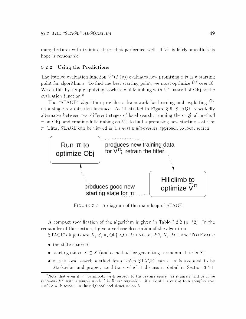
x3.2 THE \STAGE" ALGORITHM 49
many features with training states that performed well. If V � is fairly smooth, this
hope is reasonable.
3.2.2 Using the Predictions
The learned evaluation function ~V �(F (x)) evaluates how promising x is as a starting
point for algorithm �. To �nd the best starting point, we must optimize ~V � over X.
We do this by simply applying stochastic hillclimbing with ~V � instead of Obj as the
evaluation function.2
The \STAGE" algorithm provides a framework for learning and exploiting ~V �
on a single optimization instance. As illustrated in Figure 3.5, STAGE repeatedly
alternates between two di�erent stages of local search: running the original method
� on Obj, and running hillclimbing on ~V � to �nd a promising new starting state for
�. Thus, STAGE can be viewed as a smart multi-restart approach to local search.
π
π~optimize V Hillclimb to
for V ; retrain the fitteroptimize ObjπRun to
starting state for
~produces new training data
produces good newπ
Figure 3.5. A diagram of the main loop of STAGE
A compact speci�cation of the algorithm is given in Table 3.2.2 (p. 52). In the
remainder of this section, I give a verbose description of the algorithm.
STAGE's inputs are X, S, �, Obj, ObjBound, F , Fit, N , Pat, and TotEvals:
� the state space X
� starting states S � X (and a method for generating a random state in S)
� �, the local search method from which STAGE learns. � is assumed to be
Markovian and proper, conditions which I discuss in detail in Section 3.4.1.
2Note that even if ~V � is smooth with respect to the feature space|as it surely will be if werepresent ~V � with a simple model like linear regression|it may still give rise to a complex costsurface with respect to the neighborhood structure on X.
50 LEARNING FOR GLOBAL OPTIMIZATION
Intuitively, it is easiest to think of the prototypical case, hillclimbing. Note
that � encapsulates the full speci�cation of the method including all its internal
parameters; for example, � = stochastic hillclimbing, rejecting equi-cost moves,
with patience 200.
� the objective function, Obj : X ! <, to be minimized
� a lower bound on Obj, ObjBound 2 < (or �1 if no bound is known). Its use
is described in step 2d below.
� a featurizer F mapping states to real-valued features, F : X ! <D
� Fit, a function approximator. Given a set of training pairs of the form f(fi1; fi2; : : : ; fiD) 7!
yig, Fit produces a real-valued function over <D which approximately �ts the
data.
� a neighborhood structure N : X ! 2X and patience parameter Pat for running
stochastic hillclimbing on ~V �
� TotEvals, the number of state evaluations allotted for this run.
STAGE's output is a single state ~x, which has the lowest Obj value of any state
evaluated during the run. It also outputs the �nal learned evaluation function ~V �,
which provides interesting insights about what combination of features led to good
performance. (If those insights apply generally to more than one problem instance,
then the learned ~V � may be pro�tably transferred, as I show in Section 6.2.)
STAGE begins by initializing x0 to a random start state. The main loop of STAGE
proceeds as follows:
Step 2a: Optimize Obj using �. From x0, run search algorithm �, producing a
search trajectory (x0; x1; x2; : : : ; xT ).
Note that we have assumed � is a proper search procedure: the trajectory is
guaranteed to terminate.
Step 2b: Train ~V �. For each point xi on the search trajectory, de�ne yi := minj=i:::T Obj(xj),
and add the pair fF (xi) 7! yig to the training set for Fit. Retrain Fit ; call the
resulting learned evaluation function ~V �.
We accumulate a training set of all states ever visited by �. The target values
yi correspond to our de�nition of V � in Equation 3.2 (p. 47). Note that for
hillclimbing-like policies � which monotonically improve Obj, yi = Obj(xT ) 8i.
Section 3.4.3 below shows how to make this step time- and space-e�cient.
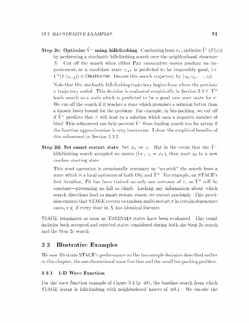
x3.3 ILLUSTRATIVE EXAMPLES 51
Step 2c: Optimize ~V � using hillclimbing. Continuing from xT , optimize ~V �(F (x))
by performing a stochastic hillclimbing search over the neighborhood structure
N . Cut o� the search when either Pat consecutive moves produce no im-
provement, or a candidate state zt+1 is predicted to be impossibly good, i.e.~V �(F (zt+1)) < ObjBound. Denote this search trajectory by (z0; z1; : : : ; zt).
Note that this stochastic hillclimbing trajectory begins from where the previous
� trajectory ended. This decision is evaluated empirically in Section 5.2.4. ~V �
leads search to a state which is predicted to be a good new start state for �.
We cut o� the search if it reaches a state which promises a solution better than
a known lower bound for the problem. For example, in bin-packing, we cut o�
if ~V � predicts that � will lead to a solution which uses a negative number of
bins! This re�nement can help prevent ~V � from leading search too far astray if
the function approximation is very inaccurate. I show the empirical bene�ts of
this re�nement in Section 5.2.5.
Step 2d: Set smart restart state. Set x0 := zt. But in the event that the ~V �
hillclimbing search accepted no moves (i.e., zt = xT ), then reset x0 to a new
random starting state.
This reset operation is occasionally necessary to \un-stick" the search from a
state which is a local optimum of both Obj and ~V �. For example, on STAGE's
�rst iteration, Fit has been trained on only one outcome of �, so ~V � will be
constant|presenting no hill to climb. Lacking any information about which
search directions lead to smart restart states, we restart randomly. This provi-
sion ensures that STAGE reverts to randommulti-restart � in certain degenerate
cases, e.g. if every state in X has identical features.
STAGE terminates as soon as TotEvals states have been evaluated. This count
includes both accepted and rejected states considered during both the Step 2a search
and the Step 2c search.
3.3 Illustrative Examples
We now illustrate STAGE's performance on the two sample domains described earlier
in this chapter, the one-dimensional wave function and the small bin-packing problem.
3.3.1 1-D Wave Function
For the wave function example of Figure 3.4 (p. 48), the baseline search from which
STAGE learns is hillclimbing with neighborhood moves of �0:1. We encode the

52 LEARNING FOR GLOBAL OPTIMIZATION
STAGE(X, S, �, Obj, ObjBound, F , Fit, N , Pat, TotEvals):Given:� a state space X� starting states S � X (and a method for generating a random state in S)� a local search procedure � that is Markovian and proper (e.g., hillclimbing)� an objective function, Obj : X ! <, to be minimized� a lower bound on Obj, ObjBound 2 < (or �1 if no bound is known)� a featurizer F mapping states to real-valued features, F : X ! <D
� a function approximator Fit� a neighborhood structure N : X ! 2X and patience parameter Pat for runningstochastic hillclimbing on ~V �
� TotEvals, the number of state evaluations allotted for this run
1. Initialize the function approximator; let x0 2 S be a random starting state forsearch.
2. Loop until number of states evaluated exceeds TotEvals:
(a) Optimize Obj using �. From x0, run search algorithm �, producing asearch trajectory (x0; x1; x2; : : : ; xT ).
(b) Train ~V �. For each point xi on the search trajectory, de�ne yi :=minj=i:::T Obj(xj), and add the pair fF (xi) 7! yig to the training set forFit. Retrain Fit ; call the resulting learned evaluation function ~V �.
(c) Optimize ~V � using hillclimbing. Continuing from xT , optimize~V �(F (x)) by performing a stochastic hillclimbing search over the neigh-borhood structure N . Cut o� the search when either Pat consecutivemoves produce no improvement, or a candidate state zt+1 is predicted tobe impossibly good, i.e. ~V �(F (zt+1)) < ObjBound. Denote this searchtrajectory by (z0; z1; : : : ; zt).
(d) Set smart restart state. Set x0 := zt. But in the event that the ~V �
hillclimbing search accepted no moves (i.e., zt = xT ), then reset x0 to anew random starting state.
3. Return the best state found.
Table 3.1. The STAGE algorithm
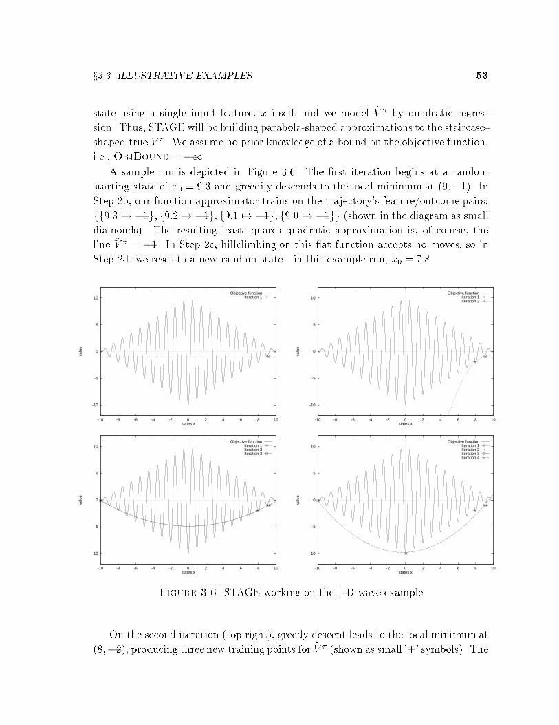
x3.3 ILLUSTRATIVE EXAMPLES 53
state using a single input feature, x itself, and we model ~V � by quadratic regres-
sion. Thus, STAGE will be building parabola-shaped approximations to the staircase-
shaped true V �. We assume no prior knowledge of a bound on the objective function,
i.e., ObjBound = �1.
A sample run is depicted in Figure 3.6. The �rst iteration begins at a random
starting state of x0 = 9:3 and greedily descends to the local minimum at (9;�1). In
Step 2b, our function approximator trains on the trajectory's feature/outcome pairs:
ff9:3 7! �1g; f9:2 7! �1g; f9:1 7! �1g; f9:0 7! �1gg (shown in the diagram as small
diamonds). The resulting least-squares quadratic approximation is, of course, the
line ~V � = �1. In Step 2c, hillclimbing on this at function accepts no moves, so in
Step 2d, we reset to a new random state|in this example run, x0 = 7:8.
-10
-5
0
5
10
-10 -8 -6 -4 -2 0 2 4 6 8 10
valu
e
states x
Objective functionIteration 1
-10
-5
0
5
10
-10 -8 -6 -4 -2 0 2 4 6 8 10
valu
e
states x
Objective functionIteration 1Iteration 2
-10
-5
0
5
10
-10 -8 -6 -4 -2 0 2 4 6 8 10
valu
e
states x
Objective functionIteration 1Iteration 2Iteration 3
-10
-5
0
5
10
-10 -8 -6 -4 -2 0 2 4 6 8 10
valu
e
states x
Objective functionIteration 1Iteration 2Iteration 3Iteration 4
Figure 3.6. STAGE working on the 1-D wave example
On the second iteration (top right), greedy descent leads to the local minimum at
(8;�2), producing three new training points for ~V � (shown as small '+' symbols). The
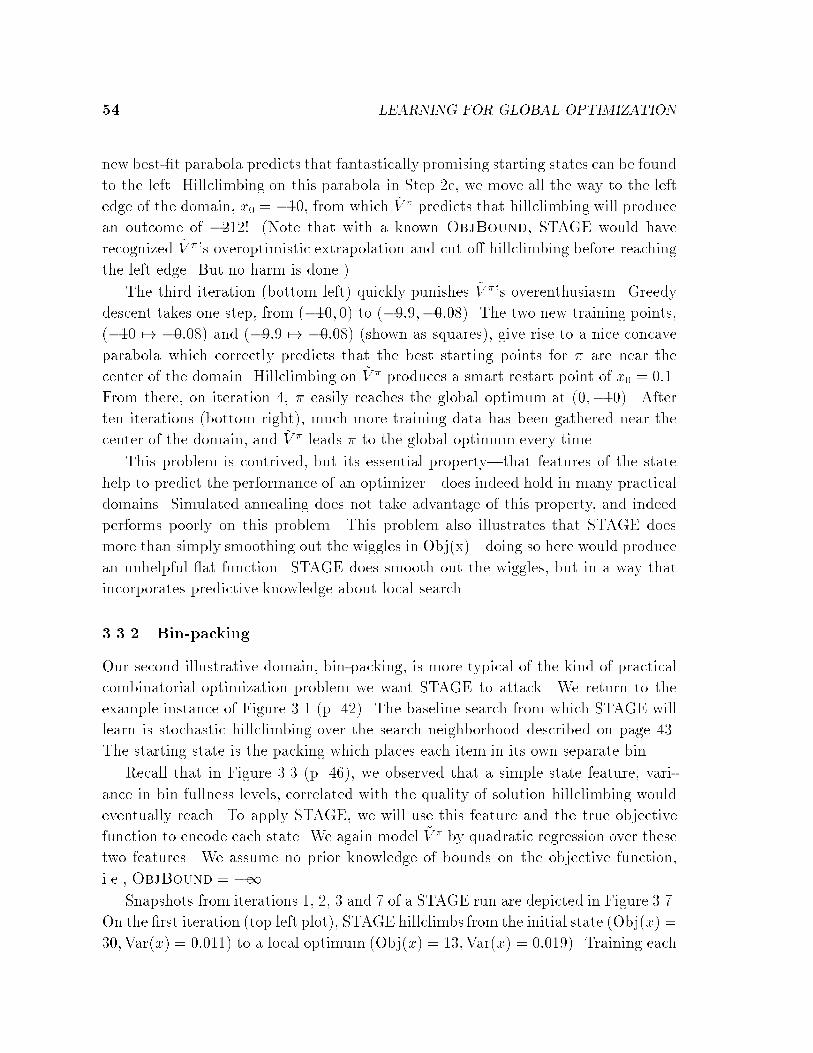
54 LEARNING FOR GLOBAL OPTIMIZATION
new best-�t parabola predicts that fantastically promising starting states can be found
to the left. Hillclimbing on this parabola in Step 2c, we move all the way to the left
edge of the domain, x0 = �10, from which ~V � predicts that hillclimbing will produce
an outcome of �212! (Note that with a known ObjBound, STAGE would have
recognized ~V �'s overoptimistic extrapolation and cut o� hillclimbing before reaching
the left edge. But no harm is done.)
The third iteration (bottom left) quickly punishes ~V �'s overenthusiasm. Greedy
descent takes one step, from (�10; 0) to (�9:9;�0:08). The two new training points,
(�10 7! �0:08) and (�9:9 7! �0:08) (shown as squares), give rise to a nice concave
parabola which correctly predicts that the best starting points for � are near the
center of the domain. Hillclimbing on ~V � produces a smart restart point of x0 = 0:1.
From there, on iteration 4, � easily reaches the global optimum at (0;�10). After
ten iterations (bottom right), much more training data has been gathered near the
center of the domain, and ~V � leads � to the global optimum every time.
This problem is contrived, but its essential property|that features of the state
help to predict the performance of an optimizer|does indeed hold in many practical
domains. Simulated annealing does not take advantage of this property, and indeed
performs poorly on this problem. This problem also illustrates that STAGE does
more than simply smoothing out the wiggles in Obj(x)|doing so here would produce
an unhelpful at function. STAGE does smooth out the wiggles, but in a way that
incorporates predictive knowledge about local search.
3.3.2 Bin-packing
Our second illustrative domain, bin-packing, is more typical of the kind of practical
combinatorial optimization problem we want STAGE to attack. We return to the
example instance of Figure 3.1 (p. 42). The baseline search from which STAGE will
learn is stochastic hillclimbing over the search neighborhood described on page 43.
The starting state is the packing which places each item in its own separate bin.
Recall that in Figure 3.3 (p. 46), we observed that a simple state feature, vari-
ance in bin fullness levels, correlated with the quality of solution hillclimbing would
eventually reach. To apply STAGE, we will use this feature and the true objective
function to encode each state. We again model ~V � by quadratic regression over these
two features. We assume no prior knowledge of bounds on the objective function,
i.e., ObjBound = �1.
Snapshots from iterations 1, 2, 3 and 7 of a STAGE run are depicted in Figure 3.7.
On the �rst iteration (top left plot), STAGE hillclimbs from the initial state (Obj(x) =
30;Var(x) = 0:011) to a local optimum (Obj(x) = 13;Var(x) = 0:019). Training each

x3.4 THEORETICAL AND COMPUTATIONAL ISSUES 55
state of that trajectory to predict the outcome 13 results in a at ~V � function (top
right). Hillclimbing on this at ~V � accepts no moves, so in Step 2d STAGE resets to
the initial state.
On the second iteration of STAGE (second row of Figure 3.7), the new stochastic
hillclimbing trajectory happens to do better than the �rst, �nishing at a local optimum
(Obj(x) = 11;Var(x) = 0:022). Our training set is augmented with target values of 11
for all states on the new trajectory. The resulting quadratic ~V � already has signi�cant
structure. Note how the contour lines of ~V �, shown on the base of the surface plot,
correspond to smoothed versions of the trajectories in our training set. Extrapolating,~V � predicts that the the best starting points for � are on arcs with higher Var(x).
STAGE hillclimbs on the learned ~V � to try to �nd a good starting point. The
trajectory, shown as a dashed line in the third plot, goes from (Obj(x) = 11;Var(x) =
0:022) up to (Obj(x) = 12;Var(x) = 0:105). Note that the search was willing to
accept some harm to the true objective function during this stage. From the new
starting state, hillclimbing on Obj does indeed lead to a yet better local optimum at
(Obj(x) = 10;Var(x) = 0:053).
During further iterations, the approximation of ~V � is further re�ned. Continuing
to alternate between standard hillclimbing on Obj (solid trajectories) and hillclimbing
on ~V �, STAGE manages to discover the global optimum at (Obj(x) = 9;Var(x) =
0) on iteration seven. STAGE's complete trajectory is plotted at the bottom left
of Figure 3.7. Contrast this STAGE trajectory with the multi-restart stochastic
hillclimbing trajectory shown in Figure 3.8, which never reached any solution better
than Obj(x) = 11.
This example illustrates STAGE's potential to exploit high-level state features
to improve performance on combinatorial optimization problems. It also illustrates
the bene�t of training ~V � on entire trajectories, not just starting states: in this run
a useful quadratic approximation was learned after only two iterations. Extensive
results on larger bin-packing instances, and on many other large-scale domains, are
presented in Chapter 4.
3.4 Theoretical and Computational Issues
STAGE is a general algorithm: it learns to predict the outcome of a local search
method � with a function approximator Fit over a feature space F . There are many
choices for �, Fit, and F . This section describes how to make those choices so that
STAGE is well-de�ned and e�cient.
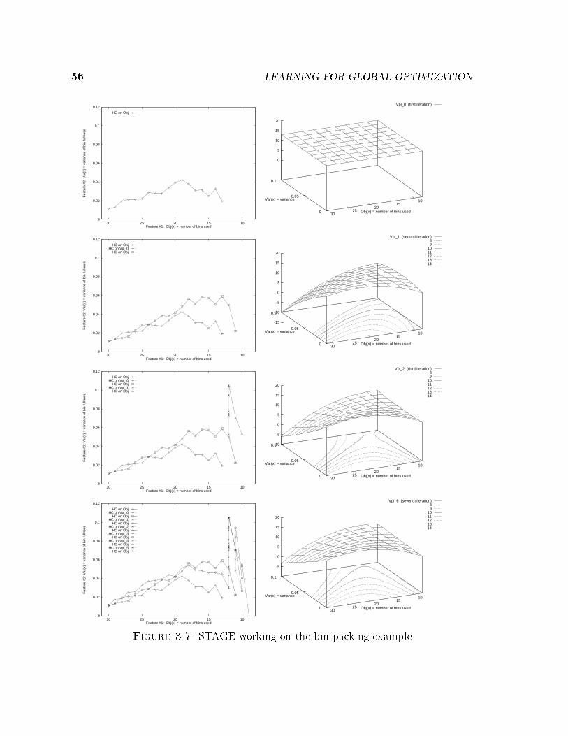
56 LEARNING FOR GLOBAL OPTIMIZATION
0
0.02
0.04
0.06
0.08
0.1
0.12
1015202530
Fea
ture
#2:
Var
(x)
= v
aria
nce
of b
in fu
llnes
s
Feature #1: Obj(x) = number of bins used
HC on Obj
Vpi_0 (first iteration)
1015
2025
300
0.05
0.1
0
5
10
15
20
Obj(x) = number of bins used
Var(x) = variance
0
0.02
0.04
0.06
0.08
0.1
0.12
1015202530
Fea
ture
#2:
Var
(x)
= v
aria
nce
of b
in fu
llnes
s
Feature #1: Obj(x) = number of bins used
HC on ObjHC on Vpi_0
HC on Obj
Vpi_1 (second iteration) 8 9
10 11 12 13 14
1015
2025
300
0.05
0.1
-15
-10
-5
0
5
10
15
20
Obj(x) = number of bins used
Var(x) = variance
0
0.02
0.04
0.06
0.08
0.1
0.12
1015202530
Fea
ture
#2:
Var
(x)
= v
aria
nce
of b
in fu
llnes
s
Feature #1: Obj(x) = number of bins used
HC on ObjHC on Vpi_0
HC on ObjHC on Vpi_1
HC on Obj
Vpi_2 (third iteration) 8 9
10 11 12 13 14
1015
2025
300
0.05
0.1-10
-5
0
5
10
15
20
Obj(x) = number of bins used
Var(x) = variance
0
0.02
0.04
0.06
0.08
0.1
0.12
1015202530
Fea
ture
#2:
Var
(x)
= v
aria
nce
of b
in fu
llnes
s
Feature #1: Obj(x) = number of bins used
HC on ObjHC on Vpi_0
HC on ObjHC on Vpi_1
HC on ObjHC on Vpi_2
HC on ObjHC on Vpi_3
HC on ObjHC on Vpi_4
HC on ObjHC on Vpi_5
HC on Obj
Vpi_6 (seventh iteration) 8 9
10 11 12 13 14
1015
2025
300
0.05
0.1
-5
0
5
10
15
20
Obj(x) = number of bins used
Var(x) = variance
Figure 3.7. STAGE working on the bin-packing example
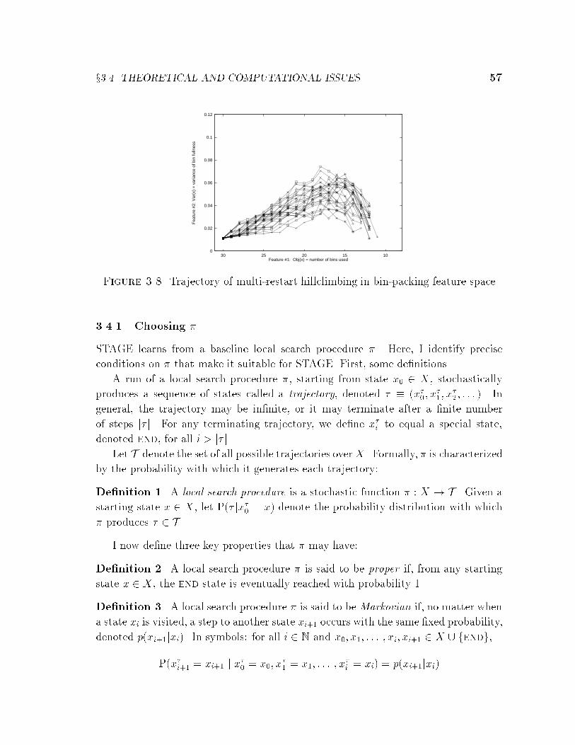
x3.4 THEORETICAL AND COMPUTATIONAL ISSUES 57
0
0.02
0.04
0.06
0.08
0.1
0.12
1015202530
Fea
ture
#2:
Var
(x)
= v
aria
nce
of b
in fu
llnes
s
Feature #1: Obj(x) = number of bins used
Figure 3.8. Trajectory of multi-restart hillclimbing in bin-packing feature space
3.4.1 Choosing �
STAGE learns from a baseline local search procedure �. Here, I identify precise
conditions on � that make it suitable for STAGE. First, some de�nitions.
A run of a local search procedure �, starting from state x0 2 X, stochastically
produces a sequence of states called a trajectory, denoted � � (x�0; x�1; x
�2; : : : ). In
general, the trajectory may be in�nite, or it may terminate after a �nite number
of steps j� j. For any terminating trajectory, we de�ne x�i to equal a special state,
denoted end, for all i > j� j.
Let T denote the set of all possible trajectories overX. Formally, � is characterized
by the probability with which it generates each trajectory:
De�nition 1. A local search procedure is a stochastic function � : X ! T . Given a
starting state x 2 X, let P(� jx�0 = x) denote the probability distribution with which
� produces � 2 T .
I now de�ne three key properties that � may have:
De�nition 2. A local search procedure � is said to be proper if, from any starting
state x 2 X, the end state is eventually reached with probability 1.
De�nition 3. A local search procedure � is said to be Markovian if, no matter when
a state xi is visited, a step to another state xi+1 occurs with the same �xed probability,
denoted p(xi+1jxi). In symbols: for all i 2 N and x0; x1; : : : ; xi; xi+1 2 X [ fendg,
P(x�i+1 = xi+1 j x�0 = x0; x
�1 = x1; : : : ; x
�i = xi) = p(xi+1jxi)

58 LEARNING FOR GLOBAL OPTIMIZATION
De�nition 4. A local search procedure � is said to be monotonic with respect to
Obj if, for every trajectory � 2 T that � can generate,
Obj(x�0) � Obj(x�1) � Obj(x�2) � � � �
If all the inequalities are strict (until perhaps reaching an end state) for every tra-
jectory, then � is called strictly monotonic.
Note that the conditions of being proper, Markovian, or monotonic are independent:
a local search procedure may satisfy none, any one, any two, or all three de�nitions.
What conditions on � make it suitable for learning by STAGE? The essence of
STAGE is to approximate the function V �(x), which predicts the expected best Obj
value on a trajectory that starts from state x and follows procedure �. Formally, we
de�ne V � as follows.
De�nition 5. For any local search procedure � and objective function Obj : X ! <,
the function V � : X ! < is de�ned by
V �(x)def= E
�inffObj(x�k) j k = 0; 1; 2; : : : g
�;
where the expectation is taken over the trajectory distribution P(� jx�0 = x).
Under one very reasonable assumption, we can show that V � is well-de�ned for
any policy �, i.e., that the expectation of De�nition 5 exists:
Proposition 1. If Obj is bounded below, then V �(x) is well-de�ned at every state
x 2 X and for all policies �.
Proof. Writing out the expectation of De�nition 5, we have
V �(x) =X�2T
P (� jx�0 = x) inffObj(x�k) j k = 0; 1; 2; : : : g:
Each trajectory's in�mum is bounded below by the assumed global bound on Obj,
and bounded above by the value of the starting state, Obj(x�0) = Obj(x). Thus,
V �(x) is a convex sum of bounded quantities, which is a well-de�ned quantity.
V � is well-de�ned for any policy �, even improper ones. However, STAGE learns
by collecting multiple sample trajectories of �; and in order for that to make sense, the
trajectories must terminate. Hence, STAGE requires that � be proper (De�nition 2).
Later in this section, I will discuss several ways of turning improper policies into
proper ones for use with STAGE.
x3.4 THEORETICAL AND COMPUTATIONAL ISSUES 59
STAGE also requires � to be Markovian. The reason for this condition is that when
� is Markovian, STAGE can use the sample trajectory data it collects much more
e�ciently. The key insight is that in any trajectory � = (x0; x1; : : : ; xi; xi+1; : : : ), each
tail of the trajectory (xi; xi+1; : : : ) is generated with exactly the same probability as
if � had started a new trajectory from xi. In other words, when � is Markovian,
every state visited is e�ectively a new starting state. This means that in Step 2b of
the STAGE algorithm (refer to page 52), STAGE can use every state of every sample
trajectory as training data for approximating V �.
Exploiting the Markov property can increase the amount of available training data
by several orders of magnitude. In practice, though, the extra training points collected
this way may be highly correlated, so it is unclear how much they will improve
optimization performance. Section 5.2.3 shows empirically that the improvement can
be substantial.
So far, we have required that � be proper for reasons of algorithmic validity and
that � be Markovian for reasons of data e�ciency. These are the only conditions
imposed by the basic STAGE algorithm of page 52. However, we can impose the
additional condition that � be monotonic, for reasons of memory e�ciency. When
� is monotonic, Markovian and proper, the in�mum in the de�nition of V � can be
rewritten as an in�nite sum:
V �(x) = E�inffObj(x�k) j k = 0; 1; 2; : : : g
�= E
�limk!1
Obj(x�k)�
(since � is monotonic)
= E
"1Xk=0
R(x�k; x�k+1)
#(since � is proper)
(3.3)
where all expectations are taken over the trajectory distribution P(� jx�0 = x), and
the additive cost function R is de�ned by
R(x; x0)def=
(Obj(x) if x 6= end and x0 = end;
0 otherwise.(3.4)
Writing V � in this form reveals that it is precisely the policy value function of
the Markov chain (X;�;R), as de�ned earlier in Section 2.1.1. This means that V �
satis�es the Bellman equations for prediction (Eq. 2.3), and all the algorithms of re-
inforcement learning apply. In particular, using the method of Least-Squares TD(�),
STAGE can learn a linear approximation to V � without ever storing a trajectory in
memory, thereby reducing memory usage signi�cantly, and with no additional com-
putational expense over supervised linear regression. The details of this technique
are given in Section 6.1.

60 LEARNING FOR GLOBAL OPTIMIZATION
We have shown that in order for STAGE to learn from a local search procedure �,
it is desirable for � to be proper, Markovian and monotonic. The remainder of this
section investigates to what extent these conditions hold, or can be made to hold, for
commonly used local search algorithms.
Steepest-descent hillclimbing. Steepest-descent takes a step from x to a neigh-
boring state x0 2 N(x) which maximally improves over Obj(x). If no neighbors
improve Obj, the trajectory terminates.
Steepest-descent is strictly monotonic. A strictly monotonic policy never visits
the same state twice on any trajectory, so if X is �nite (as is the case with com-
binatorial optimization problems), steepest-descent is guaranteed to terminate.
Steepest-descent is also clearly Markovian: at a local optimum it terminates
deterministically, and from any other state it steps with equal probability to
any x0 2 N(x) for which Obj(x0) = minz2N(x)Obj(z).
Thus, steepest-descent procedures are strictly monotonic, Markovian, and (if X
is �nite) proper.
Stochastic hillclimbing. For search problems where the neighborhoods N(x) are
large, stochastic hillclimbing is cheaper to run than steepest-descent. We con-
sider �rst the case where equi-cost moves are rejected, that is, a move from x
to x0 is accepted only if x0 belongs to the set G(x)def= fg 2 N(x) : Obj(g) �
Obj(x)g. Let HC represent this procedure for a given state space X, neighbor-
hood function N , objective function Obj, and patience value Pat.
HC is strictly monotonic. As above, assuming X is �nite, HC is guaranteed to
terminate. HC is also Markovian, with the following transition probabilities:
p(endjx) =�jN(x)j�jG(x)j
jN(x)j
�Patp(x0jx) =
(1
jG(x)j
�1 � p(endjx)
�if x0 2 G(x)
0 if x0 =2 G(x) [ fendg.
These transition probabilities assume that all neighbors are equally likely to
be sampled; it is straightforward to reweight them in the case of non-uniform
sampling distributions.
However, if we drop the assumption of rejecting equi-cost moves, stochastic hill-
climbing with patience-based termination is no longer Markovian. The reason
is that after an equi-cost move, the patience counter is not reset to zero, so
p(endjx) is not �xed but rather depends on the previous states visited. Possi-
bility 3 listed in the next paragraph describes a remedy.
x3.4 THEORETICAL AND COMPUTATIONAL ISSUES 61
Biased random walks. This general category includes any local search procedure
where state transitions are memoryless: stochastic hillclimbing with or without
equi-cost moves; force-best-move; GSAT and WALKSAT; and random walks in
the state space X. These procedures are Markovian over X but, in general,
not proper. To make them proper, a termination condition must be speci�ed.
I consider three possibilities:
Possibility 1: Run the procedure for a �xed number of steps.
This destroys the Markov condition, since the termination probability
p(endjx) depends not just on x but on the global step counter. It is
possible, however, to include this counter as part of the state, as I will
discuss under the heading of Simulated Annealing below.
Possibility 2: Introduce a termination probability � > 0.
If p(endjx) � � for every state x, then the procedure remains Markovian
and becomes proper, thus making it suitable for STAGE. However, this
approach may randomly cause termination to occur during a fruitful part
of the search trajectory.
Possibility 3: Use patience-based termination and the best-so-far abstraction.
This approach means cutting o� search after Pat consecutive steps have
failed to improve on the best state found so far on the trajectory. This
makes the search procedure proper if jXj is �nite, but breaks the Markov
property, since p(endjx) depends on not just x but also the current pa-
tience counter and the best Obj value seen previously. However, we can
use a simple trick to reclaim the Markov property.
De�nition 6. Given a local search procedure �, the best-so-far abstraction
of this policy is a new policy bsf(�) which �lters out all but the best-
so-far states on each trajectory produced by �. That is, if � produces
� = (x�0; x�1; x
�2; : : : ) with probability P (� jx�0 = x0), then with that same
probability, bsf(�) produces
� 0 = (x�i0; x�i1; x�i2; : : : )
where (i0; i1; i2; : : : ) is the subsequence consisting of all indices that satisfy
Obj(xik) < minfj:0�j<ikg
Obj(xj)
62 LEARNING FOR GLOBAL OPTIMIZATION
For example, given a trajectory of � with associated Obj values:
x0; x1; x2; x3; x4; x5; x6; x7; x8; end# # # # # # # # #42; 44; 39; 31; 35; 31; 40; 28; 30
the procedure bsf(�) would produce the monotonic trajectory
x0; x2; x3; x7; end# # # #42; 39; 31; 28
Given this de�nition, we can prove the following:
Proposition 2. If local search procedure � is Markovian over a �nite state
space X, and �0 is the procedure that results by adding patience-based ter-
mination to �, then procedure bsf(�0) is proper, Markovian, and strictly
monotonic.
The proof is given in Appendix A.1. In practical terms, this means we can
run STAGE just as described on page 52, except that in Step 2b, we train
the �tter on only the best-so-far states of each sample trajectory. Com-
pared with random termination (Possibility 2), patience-based termination
vastly reduces the number of training samples we collect for �tting V �, but
gives us both a more natural cuto� criterion and the monotonicity needed
to apply reinforcement-learning methods. In Section 4.7, I compare these
two possibilities empirically on the domain of Boolean satis�ability.
Simulated annealing. The steps taken during simulated annealing search depend
on not only the current state but also a time-varying temperature parameter
ti > 0. In particular, from state xi at time i, simulated annealing evaluates a
random neighbor x0 2 N(xi) and sets
xi+1 :=
8><>:end if i > TotEvals
x0 if rand < e[Obj(xi)�Obj(x0)]=ti
xi otherwise
(3.5)
where rand is a random variable uniformly chosen from [0; 1). The temperature
ti decreases over time. At high temperatures, moves that worsen the objective
function even by quite a lot are often accepted, whereas at low temperatures,
worsening moves are usually rejected. Improving moves and equi-cost moves
are always accepted no matter what the temperature.

x3.4 THEORETICAL AND COMPUTATIONAL ISSUES 63
Because of the dependence on temperature, simulated annealing is not Marko-
vian. However, any local search procedure can be made Markovian by aug-
menting the state space with whatever extra variables are relevant to future
transition probabilities. In the case of simulated annealing, if the temperature
schedule ti is �xed in advance, it su�ces to augment X with a single variable
i 2 N, the move counter. For example, if � uses the schedule
ti :=
(2:0 � i=1000 if i < 1000
0:99(i�1000) if i � 1000;
which decays the temperature linearly and then exponentially, then � is Marko-
vian inX�N. In the expanded space, V �(x; i) predicts the outcome of simulated
annealing when search starts from state x at time i.
However, this formulation is of limited usefulness to STAGE. For any �xed x, we
expect the best value of V � to occur at i = 0, since search should always bene�t
from having more time remaining. Thus, in Step 2c, STAGE can �x i = 0 while
searching for a good starting point; but then there is little bene�t in having
trained on all the simulated annealing trajectory states with i > 0. In other
words, it would seem that to apply the basic STAGE algorithm to simulated
annealing, one may as well train on only the actual starting state x0 of each
trajectory, and forego the improved data e�ciency that the Markov assumption
usually brings. I test this empirically in Section 5.2.3. Later, in Section 8.2.2, I
also discuss a modi�ed version of STAGE which allows simulated annealing to
exploit V � more fully.
This section has analyzed a variety of hillclimbing and random-walk local search
procedures from which STAGE can learn. From a theoretical point of view, the ideal
procedure should be proper, Markovian, and monotonic. From a practical point of
view, the procedure should also be (1) e�ective at �nding good solutions on its own,
so STAGE begins from a high performance baseline; and (2) predictable, so that V �
has learnable structure. In practice, stochastic hillclimbing rejecting equi-cost moves
seems to be a good choice; it is used for the bulk of the results in Chapter 4. Alter-
native choices for � are explored in Section 4.7 (� = WALKSAT) and Section 5.2.3
(� = simulated annealing).
3.4.2 Choosing the Features
STAGE approximates V � with statistical regression over a real-valued feature rep-
resentation of the state space X, ~V �(F (x)) � V �(x). Clearly, the quality of the

64 LEARNING FOR GLOBAL OPTIMIZATION
approximation will depend on the feature representation we choose. As with any
function approximation task, the features are \usually handcrafted, based on what-
ever human intelligence, insight, or experience is available, and are meant to capture
the most important aspects of the current state" [Bertsekas and Tsitsiklis 96].
As discussed earlier in Section 3.1.3, most practical problems are awash in features
that could help predict the outcome of local search. In the bin-packing example
of Section 3.1.3, we listed half a dozen plausible features, such as variance in bin
fullness. For a travelling salesperson problem, some reasonable features of a tour x
might include
� Obj(x) = the sum of the intercity distances in x
� the variance of the distances in x. (This could identify whether tours with some
short and some long hops are more or less promising than tours with mostly
medium-length hops.)
� the number of improving steps in the search neighborhood of x. (The general
usefulness of this feature as a local search heuristic has been investigated by
[Moll et al. 97].)
� for each city c, the distance to the next city c0 assigned by x. (These �ne-
grained features nearly specify x completely, but may be too numerous for
e�cient learning.)
� geometric features of the tour (if applicable), such as the average bend angle at
each city or average �x and �y of the distances in x.
Empirically, STAGE seems to do at least as well as random multi-restart � no
matter what features are chosen. Note that if no features are used, ~V � is always
constant, and STAGE reduces to random multi-restart �. I generally choose just
a few coarse, simple-to-compute features of a problem space, such as the variance
features mentioned above or subcomponents of the objective function. Using only a
few features minimizes the computational overhead of training ~V �, and works well in
practice. Chapter 4 gives many more examples of e�ective feature sets for large-scale
domains, and Section 5.2.1 investigates the empirical e�ect of using di�erent feature
sets.
3.4.3 Choosing the Fitter
STAGE relies on a function approximator Fit to produce ~V � from sample training
data. Examples of function approximators include polynomial regression; memory-
based methods such as k-nearest-neighbor and locally weighted regression [Cleveland
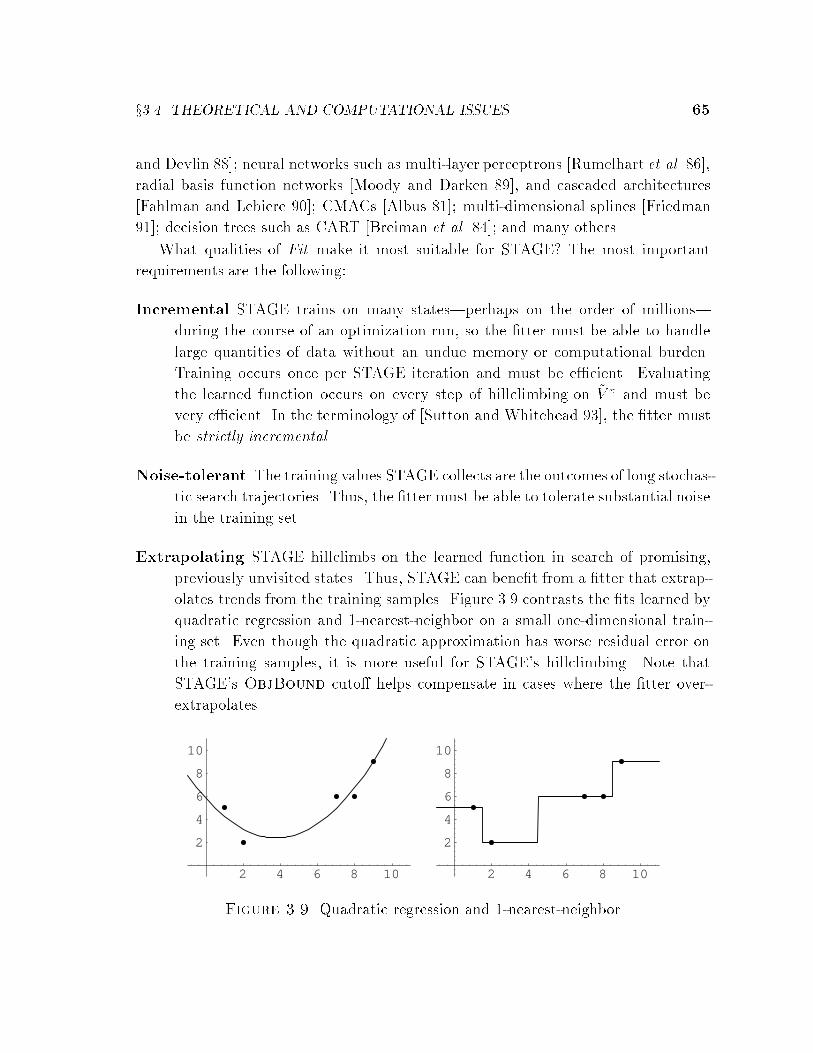
x3.4 THEORETICAL AND COMPUTATIONAL ISSUES 65
and Devlin 88]; neural networks such as multi-layer perceptrons [Rumelhart et al. 86],
radial basis function networks [Moody and Darken 89], and cascaded architectures
[Fahlman and Lebiere 90]; CMACs [Albus 81]; multi-dimensional splines [Friedman
91]; decision trees such as CART [Breiman et al. 84]; and many others.
What qualities of Fit make it most suitable for STAGE? The most important
requirements are the following:
Incremental STAGE trains on many states|perhaps on the order of millions|
during the course of an optimization run, so the �tter must be able to handle
large quantities of data without an undue memory or computational burden.
Training occurs once per STAGE iteration and must be e�cient. Evaluating
the learned function occurs on every step of hillclimbing on ~V � and must be
very e�cient. In the terminology of [Sutton and Whitehead 93], the �tter must
be strictly incremental.
Noise-tolerant The training values STAGE collects are the outcomes of long stochas-
tic search trajectories. Thus, the �tter must be able to tolerate substantial noise
in the training set.
Extrapolating STAGE hillclimbs on the learned function in search of promising,
previously unvisited states. Thus, STAGE can bene�t from a �tter that extrap-
olates trends from the training samples. Figure 3.9 contrasts the �ts learned by
quadratic regression and 1-nearest-neighbor on a small one-dimensional train-
ing set. Even though the quadratic approximation has worse residual error on
the training samples, it is more useful for STAGE's hillclimbing. Note that
STAGE's ObjBound cuto� helps compensate in cases where the �tter over-
extrapolates.
2 4 6 8 10
2
4
6
8
10
2 4 6 8 10
2
4
6
8
10
Figure 3.9. Quadratic regression and 1-nearest-neighbor
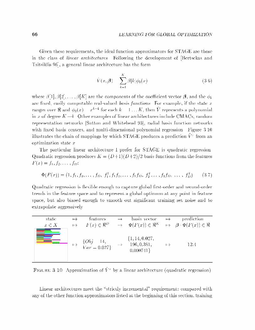
66 LEARNING FOR GLOBAL OPTIMIZATION
Given these requirements, the ideal function approximators for STAGE are those
in the class of linear architectures. Following the development of [Bertsekas and
Tsitsiklis 96], a general linear architecture has the form
~V (x;�) =
KXk=1
�[k]�k(x) (3.6)
where �[1]; �[2]; : : : ; �[K] are the components of the coe�cient vector �, and the �kare �xed, easily computable real-valued basis functions. For example, if the state x
ranges over < and �k(x) = xk�1 for each k = 1 : : :K, then ~V represents a polynomial
in x of degree K�1. Other examples of linear architectures include CMACs, random
representation networks [Sutton and Whitehead 93], radial basis function networks
with �xed basis centers, and multi-dimensional polynomial regression. Figure 3.10
illustrates the chain of mappings by which STAGE produces a prediction ~V � from an
optimization state x.
The particular linear architecture I prefer for STAGE is quadratic regression.
Quadratic regression produces K = (D+1)(D+2)=2 basis functions from the features
F (x) = f1; f2; : : : ; fD:
�(F (x)) = (1; f1; f2; : : : ; fD; f21 ; f1f2; : : : ; f1fD; f
22 : : : ; f2fD; : : : ; f
2D) (3.7)
Quadratic regression is exible enough to capture global �rst-order and second-order
trends in the feature space and to represent a global optimum at any point in feature
space, but also biased enough to smooth out signi�cant training set noise and to
extrapolate aggressively.
state 7! features 7! basis vector 7! predictionx 2 X 7! F (x) 2 <D 7! �(F (x)) 2 <K 7! � � �(F (x)) 2 <
13 12 11 10 9 8 7 6 5 4 3 2 1 0
7!fObj = 14;V ar = 0:027g
7!f1; 14; 0:027;196; 0:381;0:000741g
7! 12:4
Figure 3.10. Approximation of ~V � by a linear architecture (quadratic regression)
Linear architectures meet the \strictly incremental" requirement: compared with
any of the other function approximators listed at the beginning of this section, training

x3.4 THEORETICAL AND COMPUTATIONAL ISSUES 67
them is very e�cient in time and memory. Let our training set be denoted by
f�(1) 7! y1;�(2) 7! y2; : : : ;�(N) 7! yNg
where �(i) = (�1(F (xi)); : : : ; �K(F (xi))) is the ith training basis vector, and yi is
the ith target output. The goal of training is to �nd coe�cients that minimize the
squared residuals between predictions and target values; that is,
�� = argmin�2<K
NXi=1
�yi � � � �(i)
�2Finding the optimal coe�cients �� is a linear least squares problem that can be solved
by e�cient linear algebra techniques. The su�cient statistics for �� are the matrix
A (of dimension K �K) and vector b (of length K), computed as follows:
A =NXi=1
�(i)�T
(i) b =NXi=1
�(i)yi (3.8)
Given this compact representation of the training set, the coe�cients of the linear �t
can be calculated as
�� = A�1b (3.9)
Singular Value Decomposition is the method of choice for inverting A, since it is
robust when A is singular [Press et al. 92].
On each iteration of STAGE, many new training samples are added to the training
set, and then the function approximator is re-trained once. With a linear architecture,
adding new training samples is simply a matter of incrementing the A matrix and b
vector of Equation 3.8. For each sample, this incurs a cost of O(K2) to compute the
outer product �(i)�T
(i) and O(K) to compute �(i)yi. The training samples can then
be discarded. Updated values of �� are computed by Equation 3.9 in O(K3) time,
independent of the number of samples in the training set.
Linear architectures also have the advantage of low memory use. Between itera-
tions of STAGE, we need store only A and b, not the whole training set. Therefore,
the bottleneck on memory usage is the space required to store the state features
along any single trajectory during Step 2a (refer to page 52). This is usually quite
modest, but can become signi�cant for local search procedures which visit tens of
thousands of states on a single trajectory. In such cases, the Least-Squares TD(1)
algorithm can be used. Least-Squares TD(1) produces the same coe�cients �� as
Equation 3.9 above with the same amount of computation, but requires no memory

68 LEARNING FOR GLOBAL OPTIMIZATION
for saving trajectories: it performs its computations fully incrementally as the trajec-
tory is generated. Least-Squares TD(1) may be applied in STAGE when the baseline
local search procedure � is monotonic; the algorithm is described in its general TD(�)
form in Section 6.1.
3.4.4 Discussion
This section has considered the theoretical and computational issues that arise in
choosing a local search procedure �, feature mapping F , and function approximator
Fit for use by STAGE. To summarize the practical conclusions of this section:
1. A good choice for � is stochastic hillclimbing, rejecting equi-cost moves, with
patience-based termination. This procedure is proper, Markovian, monotonic,
and easy to apply in almost any domain.
2. Features F (x) of a state x must be hand chosen, but are generally abundant.
A good choice is to use a few simple, coarse features such as subcomponents of
Obj(x).
3. A good choice for Fit is quadratic regression. Its training time and memory
requirements are small and independent of the number of training samples.
STAGE has two further inputs that have not yet been discussed: N and Pat,
the neighborhood structure and patience parameter used for stochastic hillclimbing
on the learned evaluation function ~V �. In general, I simply set these to the same
neighborhood structure and patience parameter which were used to de�ne �.

69
Chapter 4
STAGE: Empirical Results
The last chapter introduced STAGE, an optimization algorithm that learns to
incorporate extra features of a problem into an evaluation function and thereby im-
prove overall performance. In this chapter, I �rst de�ne my methodology for measur-
ing STAGE's performance and comparing it to other algorithms empirically. I then
describe my implementations of seven large-scale optimization domains with widely
varying characteristics:
� Bin-packing (x4.2): pack a collection of items into as few bins as possible|
the classic NP-complete problem, as discussed in the examples of Chapter 3;
� Channel routing (x4.3): minimize the area needed to produce a speci�ed
circuit in VLSI;
� Bayes net structure-�nding (x4.4): determine the optimal graph of data
dependencies between variables in a dataset;
� Radiotherapy treatment planning (x4.5): given an anatomical map of a
patient's brain tumor and nearby sensitive structures, plan a minimally harmful
radiation treatment;
� Cartogram design (x4.6): for geographic visualization purposes, redraw a
map of the United States so that each state's area is proportional to its popu-
lation, minimizing deformations;
� Satis�ability (x4.7): given a Boolean formula, �nd a variable assignment that
makes the formula true; and
� Boggle board setup (x4.8): �nd a 5 � 5 grid of letters containing as many
English words in connected paths as possible.
For each of these domains, I apply STAGE as described in Section 3.2, unmodi�ed,
and report statistically signi�cant results.

70 STAGE: EMPIRICAL RESULTS
4.1 Experimental Methodology
The e�ectiveness of a heuristic optimization algorithm should be measured along
three main dimensions [Barr et al. 95,Johnson 96]:
� Solution quality. How close are the solutions found by the method to opti-
mality?
� Computational e�ort. How long did the method take to �nd its best solu-
tion? How quickly does it �nd good solutions?
� Robustness. Does the method work across multiple problem instances and
varying domains? In the case of a randomized method, are its results consistent
when applied repeatedly to the same problem?
This chapter evaluates the performance of STAGE in each of these dimensions through
a statistical analysis of the results of thousands of experimental runs. STAGE's results
are contrasted to the optimal solution (if available), special-purpose algorithms for
each domain (if available), and two general-purpose reference algorithms: multiple-
restart stochastic hillclimbing and simulated annealing.
4.1.1 Reference Algorithms
I compare STAGE's performance to that of multi-restart stochastic hillclimbing and
simulated annealing on every problem instance. Multi-restart stochastic hillclimbing
is not only straightforward to implement, but also a surprisingly e�ective heuristic
on some domains. For example, hillclimbing with 100 random restarts is gener-
ally adequate for �nding high-quality solutions to a geometric line-matching prob-
lem [Beveridge et al. 96]. For the comparative experiments of this chapter, I run
hillclimbing with the following parameters:
� At each step, moves are randomly chosen in a problem-dependent way. The
�rst such move that either improves Obj or keeps it the same is accepted.
� The patience parameter is set individually for each problem; generally the best
setting is on the same order of magnitude as the number of available actions.
Search restarts whenever patience consecutive moves have been evaluated since
�nding the state whose objective function value is best on the current trajectory.
� Search restarts at either a special start state or a random state; this distribution
is also set individually for each domain.
x4.1 EXPERIMENTAL METHODOLOGY 71
� The total number of moves evaluated is limited to TotEvals, the same pa-
rameter that governs STAGE's termination.
Conceptually, simulated annealing is only slightly more complicated: it accepts
all improving and equi-cost moves, but also probabilistically accepts some worsening
moves. In practice, though, implementing an e�ective temperature annealing schedule
which regulates the evolution of the acceptance probabilities can be di�cult. Based
on a review of the literature and a good deal of experimentation, I implemented
Swartz's modi�cation of the Lam temperature schedule [Swartz and Sechen 90,Lam
and Delosme 88]. This adaptive schedule produces excellent results across a variety of
domains. Appendix B provides detailed justi�cation for and implementation details
of this \modi�ed Lam" schedule.
4.1.2 How the Results are Tabulated
For the purpose of summarizing the solution quality, computational e�ort, and robust-
ness of STAGE and competing heuristics, it would be ideal to plot each algorithm's
average performance versus elapsed time. However, my experiments were run on
a pool of over 100 workstations having widely varying job loads, processor speeds,
and system architectures; collecting meaningful average timing measurements was
therefore impossible. Instead, for each algorithm I plot average performance ver-
sus number of moves considered. In practical applications where evaluating Obj is
relatively costly, this quantity correlates strongly with total running time, yet is inde-
pendent of machine speed and load. I also do give sample timing comparisons on each
domain, measured on an SGI Indigo2 R10000 workstation, but since this workstation
is multi-user, these �gures should be considered very rough. Each time reported is
the median of three independent runs.
Note that for STAGE, the number of moves considered includes moves made
during both stages of the algorithm, i.e., both running � and optimizing ~V �. However,
this number does not capture STAGE's additional overhead for feature construction
and function approximator training. With linear approximation architectures (see
Section 3.4.3) and simple features, this overhead is minimal|typically, less than 10%
of the execution time.
On any single run of a search algorithm, after n moves have been considered, the
performance is de�ned as the best Obj value found up to that point. The overall
performance of the algorithm at time n, Q(n), is de�ned as the expected single-run
performance:
Q(n)def= E
�mini=0:::n
Obj(xi)
72 STAGE: EMPIRICAL RESULTS
where the expectation is taken over all trajectories (x0; x1; : : : ) that the algorithm
may generate on the problem. For experimental evaluation purposes, I sample Q(n)
by taking the mean best value seen over multiple independent runs. The variable n
ranges from 0 to TotEvals. Note that Q(n) is non-increasing regardless of whether
the search algorithm monotonically improves Obj.
Figure 4.1 illustrates how a performance curve is produced for an algorithm and
a problem. In this example, a search algorithm is run �ve times for TotEvals =
500 steps each run. The upper-left graph plots the objective function value of the
states visited during the course of these �ve runs. The upper-right graph plots the
performance of each run, that is, the best Obj value seen so far at each step. The third
graph, at bottom left, plots the mean performance of the �ve runs over time. Finally,
the fourth graph summarizes the algorithm's overall performance in a boxplot. The
boxplot is calculated at the endpoint of the runs, where n = TotEvals. It gives the
95% con�dence interval of the mean performance (shown as a box around the mean)1
and the end result of the best and worst of the runs (shown as \whiskers").
For each comparative experiment in this chapter, the results are presented in two
�gures and a table:
� a mean performance curve, like the lower left graph of Figure 4.1, indicates how
quickly each algorithm reached its best performance level;
� a boxplot, like the lower right graph of Figure 4.1, provides a useful visual means
for comparing the algorithms against one another [Barr et al. 95]; and
� a results table numerically displays the same data as the boxplot. In each table,
the best minimum, best maximum, and statistically best mean performances
are boldfaced. Each table also reports the running time and overall percentage
of moves acceptedTotEvals
for each algorithm, but these �gures are medians of only three
runs and should thus be considered rough estimates.
I now proceed to describe the various optimization domains, experiments, and
results by which I have evaluated STAGE.
4.2 Bin-packing
Bin-packing, a classical NP-hard optimization problem [Garey and Johnson 79],
has often been used as a testbed for combinatorial optimization algorithms (e.g.,
1The 95% con�dence interval of the mean is simply 2 standard errors on either side: �� 2�pN.

x4.2 BIN-PACKING 73
5
10
15
20
25
30
35
40
45
0 50 100 150 200 250 300 350 400 450 500
Obj
ectiv
e fu
nctio
n
Number of moves considered
Run 1Run 2Run 3Run 4Run 5
5
10
15
20
25
30
35
40
45
0 50 100 150 200 250 300 350 400 450 500
Number of moves considered
Run 1 best-so-farRun 2 best-so-farRun 3 best-so-farRun 4 best-so-farRun 5 best-so-far
5
10
15
20
25
30
35
40
45
0 50 100 150 200 250 300 350 400 450 500
Obj
ectiv
e fu
nctio
n
Number of moves considered
Average best-so-far
5
10
15
20
25
30
35
40
45
Boxplot of algorithm performance at n=500
Figure 4.1. From a number of independent runs of an algorithm (upper left) andtheir best-so-far curves (upper right), a single performance curve (lower left) and boxplot (lower right) are generated to summarize the algorithm's performance. Pleaserefer to the text for a detailed explanation.
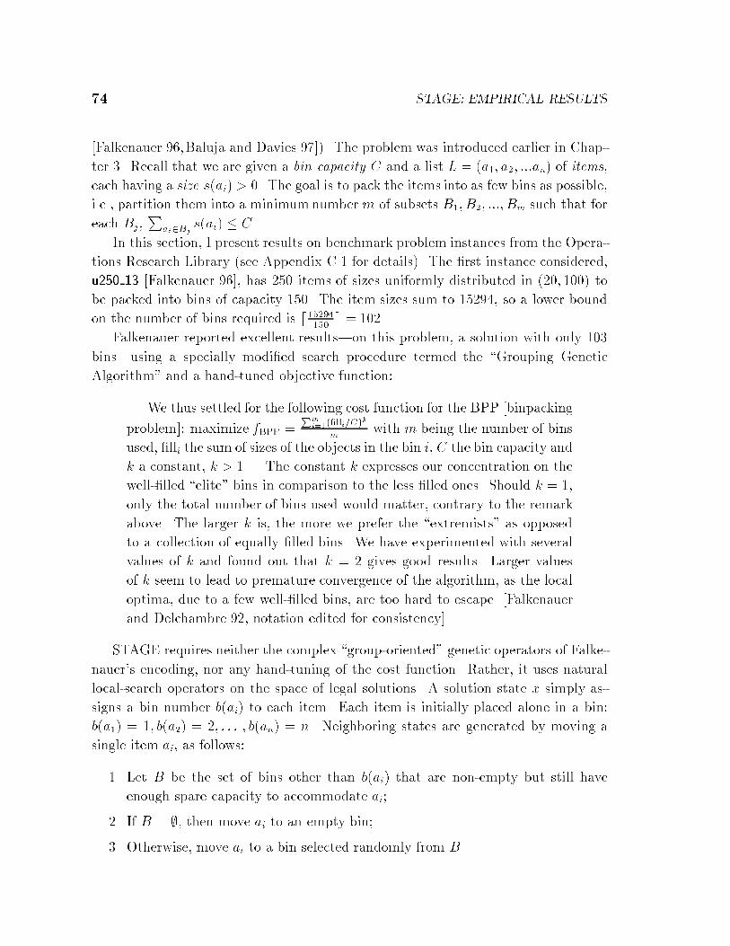
74 STAGE: EMPIRICAL RESULTS
[Falkenauer 96,Baluja and Davies 97]). The problem was introduced earlier in Chap-
ter 3. Recall that we are given a bin capacity C and a list L = (a1; a2; :::an) of items,
each having a size s(ai) > 0. The goal is to pack the items into as few bins as possible,
i.e., partition them into a minimum number m of subsets B1; B2; :::; Bm such that for
each Bj,P
ai2Bjs(ai) � C.
In this section, I present results on benchmark problem instances from the Opera-
tions Research Library (see Appendix C.1 for details). The �rst instance considered,
u250 13 [Falkenauer 96], has 250 items of sizes uniformly distributed in (20; 100) to
be packed into bins of capacity 150. The item sizes sum to 15294, so a lower bound
on the number of bins required is d15294150
e = 102.
Falkenauer reported excellent results|on this problem, a solution with only 103
bins|using a specially modi�ed search procedure termed the \Grouping Genetic
Algorithm" and a hand-tuned objective function:
We thus settled for the following cost function for the BPP [binpacking
problem]: maximize fBPP =Pm
i=1(�lli=C)k
mwith m being the number of bins
used, �lli the sum of sizes of the objects in the bin i, C the bin capacity and
k a constant, k > 1.... The constant k expresses our concentration on the
well-�lled \elite" bins in comparison to the less �lled ones. Should k = 1,
only the total number of bins used would matter, contrary to the remark
above. The larger k is, the more we prefer the \extremists" as opposed
to a collection of equally �lled bins. We have experimented with several
values of k and found out that k = 2 gives good results. Larger values
of k seem to lead to premature convergence of the algorithm, as the local
optima, due to a few well-�lled bins, are too hard to escape. [Falkenauer
and Delchambre 92, notation edited for consistency]
STAGE requires neither the complex \group-oriented" genetic operators of Falke-
nauer's encoding, nor any hand-tuning of the cost function. Rather, it uses natural
local-search operators on the space of legal solutions. A solution state x simply as-
signs a bin number b(ai) to each item. Each item is initially placed alone in a bin:
b(a1) = 1; b(a2) = 2; : : : ; b(an) = n. Neighboring states are generated by moving a
single item ai, as follows:
1. Let B be the set of bins other than b(ai) that are non-empty but still have
enough spare capacity to accommodate ai;
2. If B = ;, then move ai to an empty bin;
3. Otherwise, move ai to a bin selected randomly from B.

x4.2 BIN-PACKING 75
Note that hillclimbing methods always reject moves of type (2), which add a new bin;
and that if equi-cost moves are also rejected, then the only accepted moves will be
those that empty a bin by placing a singleton item in an occupied bin.
The objective function STAGE is given to minimize is simply Obj(x) = m, the
number of bins used. There is no need to tune the evaluation function manually. For
automatic learning of its own secondary evaluation function, STAGE is provided with
two state features, just as in the bin-packing example of section 3.3.2 (p. 54):
� Feature 1: Obj(x), the number of bins used by solution x
� Feature 2: Var(x), the variance in bin fullness levels
This second feature provides STAGE with information about the proportion of \ex-
tremist" bins, similar to that provided by Falkenauer's cost function. STAGE then
learns its evaluation function by quadratic regression over these two features.
The remaining parameters to STAGE are set as follows: the patience parameters
are set to 250 and the ObjBound cuto� is disabled (set to �1). In a few informal
experiments, varying these parameters had a negligible e�ect on the results. Table 4.1
lists all of STAGE's parameter settings.
Parameter Setting
� stochastic hillclimbing, rejecting equi-cost moves, patience=250ObjBound �1features 2 (number of bins used, variance of bin fullness levels)�tter quadratic regressionPat 250TotEvals 100,000
Table 4.1. Summary of STAGE parameters for bin-packing results. (For descrip-tions of the parameters, see Section 3.2.2.)
STAGE's performance is contrasted with that of four other algorithms:
� HC0: multi-restart stochastic hillclimbing with equi-cost moves rejected, pa-
tience=1000. On each restart, search begins at the initial state which has each
item in its own bin.
� HC1: the same, but with equi-cost moves accepted.
� SA: simulated annealing, as described in Appendix B.
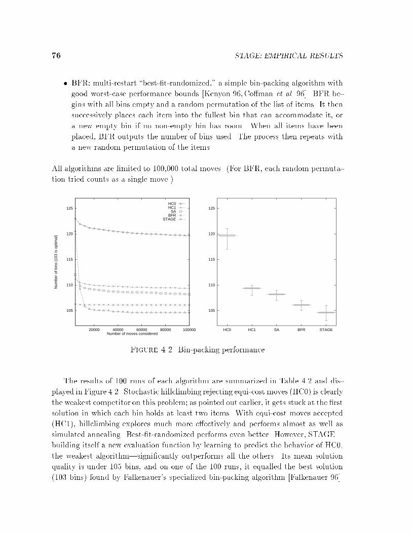
76 STAGE: EMPIRICAL RESULTS
� BFR: multi-restart \best-�t-randomized," a simple bin-packing algorithm with
good worst-case performance bounds [Kenyon 96,Co�man et al. 96]. BFR be-
gins with all bins empty and a random permutation of the list of items. It then
successively places each item into the fullest bin that can accommodate it, or
a new empty bin if no non-empty bin has room. When all items have been
placed, BFR outputs the number of bins used. The process then repeats with
a new random permutation of the items.
All algorithms are limited to 100,000 total moves. (For BFR, each random permuta-
tion tried counts as a single move.)
105
110
115
120
125
20000 40000 60000 80000 100000
Num
ber
of b
ins
(103
is o
ptim
al)
Number of moves considered
HC0HC1
SABFR
STAGE
105
110
115
120
125
HC0 HC1 SA BFR STAGE
Figure 4.2. Bin-packing performance
The results of 100 runs of each algorithm are summarized in Table 4.2 and dis-
played in Figure 4.2. Stochastic hillclimbing rejecting equi-cost moves (HC0) is clearly
the weakest competitor on this problem; as pointed out earlier, it gets stuck at the �rst
solution in which each bin holds at least two items. With equi-cost moves accepted
(HC1), hillclimbing explores much more e�ectively and performs almost as well as
simulated annealing. Best-�t-randomized performs even better. However, STAGE|
building itself a new evaluation function by learning to predict the behavior of HC0,
the weakest algorithm|signi�cantly outperforms all the others. Its mean solution
quality is under 105 bins, and on one of the 100 runs, it equalled the best solution
(103 bins) found by Falkenauer's specialized bin-packing algorithm [Falkenauer 96].

x4.2 BIN-PACKING 77
The best-so-far curves show that STAGE learns quickly, achieving good performance
after only about 10000 moves, or about 4 iterations on average.
STAGE's timing overhead for learning was on the order of only 7% over HC0.
In fact, the timing di�erences between SA, HC1, HC0, and STAGE are attributable
mainly to their di�erent ratios of accepted to rejected moves: rejected moves are
slower in my bin-packing implementation since they must be undone. Since SA ac-
cepts most moves it considers early in search, it �nishes slightly more quickly. The
BFR runs took much longer, but the performance curve makes it clear that its best
solutions were reached quickly.2
Instance Algorithm Performance (100 runs each) � moves
mean best worst time accepted
u250 13 HC0 119.68�0.17 117 121 12.4s 8%HC1 109.38�0.10 108 110 11.4s 71%SA 108.19�0.09 107 109 11.1s 44%BFR 106.10�0.07 105 107 95.3s |STAGE 104.60�0.11 103 106 13.3s 6%
Table 4.2. Bin-packing results
As a follow-up experiment, I ran HC1, SA, BFR, and STAGE on all 20 bin-packing
problem instances in the u250 class of the OR-Library (see Appendix C.1). All runs
used the same settings shown in Table 4.1. The results, given in Table 4.3, show
that STAGE consistently found the best packings in each case. STAGE's average
improvements over HC1, SA, and BFR were 5:0�0:3 bins, 3:8�0:3 bins, and 1:6�0:3
bins, respectively.
How did STAGE succeed? The STAGE runs followed the same pattern as the runs
on the small example bin-packing instance of last chapter (x3.3.2). STAGE learned a
secondary evaluation function, ~V �, that successfully traded o� between the original
objective and the additional bin-variance feature to identify promising start states.
A typical evaluation function learned by STAGE is plotted in Figure 4.3.3 As in
2Falkenauer reported a running time of 6346 seconds for his genetic algorithm to �nd the globaloptimum on this instance [Falkenauer 96], though this was measured on an SGI R4000 and our timeswere measured on an SGI R10000.
3The particular ~V � plotted is a snapshot from iteration #15 of a STAGE run, immediately afterthe solution Obj(x) = 103 was found. The learned coe�cients are
~V �(Obj;Var) = �99:1 + 636 Var + 3462 Var2 + 2:64 Obj� 9:03 Obj �Var� 0:00642 Obj2:
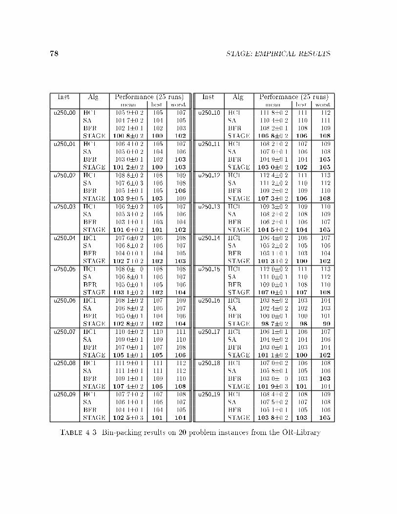
78 STAGE: EMPIRICAL RESULTS
Inst. Alg. Performance (25 runs)mean best worst
u250 00 HC1 105.9�0.2 105 107SA 104.7�0.2 104 105BFR 102.1�0.1 102 103STAGE 100.8�0.2 100 102
u250 01 HC1 106.4�0.2 105 107SA 105.0�0.2 104 106BFR 103.0�0.1 102 103
STAGE 101.2�0.2 100 103
u250 02 HC1 108.8�0.2 108 109SA 107.6�0.3 106 108BFR 105.1�0.1 105 106
STAGE 103.9�0.5 103 109u250 03 HC1 106.2�0.2 105 107
SA 105.3�0.2 105 106BFR 103.1�0.1 103 104STAGE 101.6�0.2 101 102
u250 04 HC1 107.6�0.2 106 108SA 106.8�0.2 106 107BFR 104.0�0.1 104 105STAGE 102.7�0.2 102 103
u250 05 HC1 108.0� 0 108 108SA 106.8�0.1 106 107BFR 105.0�0.1 105 106STAGE 103.1�0.2 102 104
u250 06 HC1 108.1�0.2 107 109SA 106.8�0.2 106 107BFR 105.0�0.1 104 106STAGE 102.8�0.2 102 104
u250 07 HC1 110.4�0.2 110 111SA 109.0�0.1 109 110BFR 107.0�0.1 107 108STAGE 105.1�0.1 105 106
u250 08 HC1 111.9�0.1 111 112SA 111.1�0.1 111 112BFR 109.1�0.1 109 110STAGE 107.4�0.2 106 108
u250 09 HC1 107.7�0.2 107 108SA 106.1�0.1 106 107BFR 104.1�0.1 104 105STAGE 102.5�0.3 101 104
Inst. Alg. Performance (25 runs)mean best worst
u250 10 HC1 111.8�0.2 111 112SA 110.4�0.2 110 111BFR 108.2�0.1 108 109STAGE 106.8�0.2 106 108
u250 11 HC1 108.2�0.2 107 109SA 107.0�0.1 106 108BFR 104.9�0.1 104 105
STAGE 103.0�0.2 102 105
u250 12 HC1 112.4�0.2 111 113SA 111.2�0.2 110 112BFR 109.2�0.2 109 110STAGE 107.3�0.2 106 108
u250 13 HC1 109.3�0.2 109 110SA 108.2�0.2 108 109BFR 106.2�0.1 106 107STAGE 104.5�0.2 104 105
u250 14 HC1 106.4�0.2 106 107SA 105.2�0.2 105 106BFR 103.1�0.1 103 104STAGE 101.3�0.2 100 102
u250 15 HC1 112.0�0.2 111 113SA 111.0�0.1 110 112BFR 109.0�0.1 108 110STAGE 107.0�0.1 107 108
u250 16 HC1 103.8�0.2 103 104SA 102.4�0.2 102 103BFR 100.0�0.1 100 101STAGE 98.7�0.2 98 99
u250 17 HC1 106.1�0.1 106 107SA 104.9�0.2 104 106BFR 103.0�0.1 103 104STAGE 101.1�0.2 100 102
u250 18 HC1 107.0�0.2 106 108SA 105.8�0.1 105 106BFR 103.0� 0 103 103
STAGE 101.9�0.3 101 104u250 19 HC1 108.4�0.2 108 109
SA 107.5�0.2 107 108BFR 105.1�0.1 105 106STAGE 103.8�0.2 103 105
Table 4.3. Bin-packing results on 20 problem instances from the OR-Library
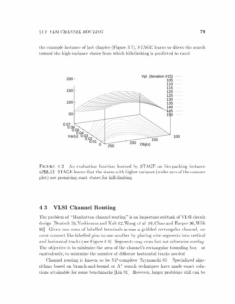
x4.3 VLSI CHANNEL ROUTING 79
the example instance of last chapter (Figure 3.7), STAGE learns to direct the search
toward the high-variance states from which hillclimbing is predicted to excel.
Vpi (iteration #15) 105 110 115 120 125 130 135 140 145 150
100150
2002500
0.010.02
0.030.04
0.050.06
0.07
50
100
150
200
Obj(x)
Var(x)
Figure 4.3. An evaluation function learned by STAGE on bin-packing instanceu250 13. STAGE learns that the states with higher variance (wider arcs of the contourplot) are promising start states for hillclimbing.
4.3 VLSI Channel Routing
The problem of \Manhattan channel routing" is an important subtask of VLSI circuit
design [Deutsch 76,Yoshimura and Kuh 82,Wong et al. 88,Chao and Harper 96,Wilk
96]. Given two rows of labelled terminals across a gridded rectangular channel, we
must connect like-labelled pins to one another by placing wire segments into vertical
and horizontal tracks (see Figure 4.4). Segments may cross but not otherwise overlap.
The objective is to minimize the area of the channel's rectangular bounding box|or
equivalently, to minimize the number of di�erent horizontal tracks needed.
Channel routing is known to be NP-complete [Szymanski 85]. Specialized algo-
rithms based on branch-and-bound or A* search techniques have made exact solu-
tions attainable for some benchmarks [Lin 91]. However, larger problems still can be

80 STAGE: EMPIRICAL RESULTS
5
7
6
7
7
9
5
8
9
0
3
4
4
5
1
3
2
4
4
6
1
2
8
9
Figure 4.4. A small channel routing instance, shown with a solution occupying 7horizontal tracks.
solved only approximately by heuristic techniques, e.g. [Wilk 96]. My implementa-
tion is based on the SACR system [Wong et al. 88, Chapter 4], a simulated annealing
approach. SACR's operator set is sophisticated, involving manipulations to a parti-
tioning of vertices in an acyclic constraint graph. If the partitioning meets certain
additional constraints, then it corresponds to a legal routing, and the number of
partitions corresponds to the channel size we are trying to minimize.
Like Falkenauer's bin-packing implementation described above, Wong's channel
routing implementation required manual objective function tuning:
Clearly, the objective function to be minimized is the channel width w(x).
However, w(x) is too crude a measure of the quality of intermediate so-
lutions. Instead, for any valid partition x, the following cost function is
used:
C(x) = w(x)2 + �p � p(x)2 + �U � U(x) (4.1)
where p(x) is the longest path length of Gx [a graph induced by the
partitioning], both �p and �U are constants, and ... U(x) =Pw(x)
i=1 ui(x)2,
where ui(x) is the fraction of track i that is unoccupied. [Wong et al. 88,
notation edited for consistency]

x4.3 VLSI CHANNEL ROUTING 81
They hand-tuned the coe�cients and set �p = 0:5; �U = 10. To apply STAGE
to this problem, I began with not the contrived function C(x) but the natural ob-
jective function Obj(x) = w(x). The additional objective function terms used in
Equation 4.1, p(x) and U(x), along with w(x) itself, were given as the three input
features to STAGE's function approximator. Thus, the features of a solution x are
� Feature 1: w(x) = channel width, i.e. the number of horizontal tracks used by
the solution.
� Feature 2: p(x) = the length of the longest path in a \merged constraint graph"
Gx representing the solution. This feature is a lower bound on the channel width
of all solutions derived from x by merging subnets [Wong et al. 88]. In other
words, this feature bounds the quality of solution that can be reached from x
by repeated application of a restricted class of operators, namely, merging the
contents of two tracks into one. The inherently predictive nature of this feature
suits STAGE well.
� Feature 3: U(x) = the sparseness of the horizontal tracks, measured byPw(x)
i=1 ui(x)2,
where ui(x) is the fraction of track i that is unoccupied. Note that this feature
is real-valued, whereas the other two are discrete; and that 0 � U(x) < w(x).
Table 4.4 summarizes the remaining STAGE parameter settings.
Parameter Setting
� stochastic hillclimbing, rejecting equi-cost moves, patience=250ObjBound �1features 3 (w(x); p(x); U(x))�tter linear regressionPat 250TotEvals 500,000
Table 4.4. Summary of STAGE parameters for channel routing results
STAGE's performance is contrasted with that of four other algorithms:
� HC0: multi-restart stochastic hillclimbing with equi-cost moves rejected, pa-
tience=400. On each restart, search begins at the initial state which has each
subnet on its own track.
� HC1: the same, but with equi-cost moves accepted.

82 STAGE: EMPIRICAL RESULTS
� SAW: simulated annealing, using the hand-tuned objective function of Equa-
tion 4.1 [Wong et al. 88].
� SA: simulated annealing, using the true objective function Obj(x) = w(x).
� HCI: stochastic hillclimbing with equi-cost moves accepted, patience=1 (i.e.,
no restarting).
All algorithms were limited to 500,000 total moves. Results on YK4, an instance
with 140 vertical tracks, are given in Figure 4.5 and Table 4.5. By construction (see
Appendix C.2 for details), the optimal routing x� for this instance occupies only 10
horizontal tracks, i.e. Obj(x�) = 10. A 12-track solution is depicted in Figure 4.6.
10
15
20
25
30
35
40
45
50
100000 200000 300000 400000 500000
Are
a of
circ
uit l
ayou
t (10
is o
ptim
al)
Number of moves considered
HC0HC1
SAWSA
HCISTAGE
10
15
20
25
30
35
40
45
50
HC0 HC1 SAW SA HCI STAGE
Figure 4.5. Channel routing performance on instance YK4
None of the local search algorithms successfully �nds an optimal 10-track solution.
Experiments HC0 and HC1 show that multi-restart hillclimbing performs terribly
when equi-cost moves are rejected, but signi�cantly better when equi-cost moves
are accepted. Experiment SAW shows that simulated annealing, as used with the
objective function of [Wong et al. 88], does considerably better. Surprisingly, the
annealer of Experiment SA does better still. It seems that the \crude" evaluation
function Obj(x) = w(x) allows a long simulated annealing run to e�ectively random-
walk along the ridge of all solutions of equal cost, and given enough time it will
fortuitously �nd a hole in the ridge. In fact, increasing hillclimbing's patience to 1
(disabling restarts) worked nearly as well.
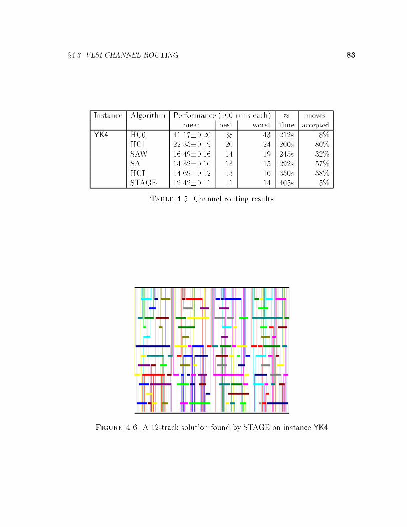
x4.3 VLSI CHANNEL ROUTING 83
Instance Algorithm Performance (100 runs each) � moves
mean best worst time accepted
YK4 HC0 41.17�0.20 38 43 212s 8%HC1 22.35�0.19 20 24 200s 80%SAW 16.49�0.16 14 19 245s 32%SA 14.32�0.10 13 15 292s 57%HCI 14.69�0.12 13 16 350s 58%STAGE 12.42�0.11 11 14 405s 5%
Table 4.5. Channel routing results
Figure 4.6. A 12-track solution found by STAGE on instance YK4

84 STAGE: EMPIRICAL RESULTS
STAGE performs signi�cantly better than all of these. How does STAGE learn
to combine the features w(x), p(x), and U(x) into a new evaluation function that
outperforms simulated annealing? I have investigated this question extensively; the
analysis is reported in Chapter 5. Later, in Section 6.2, I also report the results of
transferring STAGE's learned evaluation function between di�erent channel routing
instances.
The disparity in the running times of the algorithm deserves explanation. The
STAGE runs took about twice as long to complete as the hillclimbing runs, but
this is not due to the overhead for STAGE's learning: linear regression over three
simple features is extremely cheap. Rather, STAGE is slower because when the search
reaches good solutions, the process of generating a legal move candidate becomes
more expensive; STAGE is victimized by its own success. STAGE and HCI are also
slowed relative to SA because they reject many more moves, forcing extra \undo"
operations. In any event, the performance curve of Figure 4.5 indicates that halving
any algorithm's running time would not a�ect its relative performance ranking.
4.4 Bayes Network Learning
Given a dataset, an important data mining task is to identify the Bayesian network
structure that best models the probability distribution of the data [Mitchell 97,Heck-
erman et al. 94, Friedman and Yakhini 96]. The problem amounts to �nding the
best-scoring acyclic graph structure on A nodes, where A is the number of attributes
in each data record.
Several scoring metrics are common in the literature, including metrics based on
Bayesian analysis [Chickering et al. 94] and metrics based on Minimum Description
Length (MDL) [Lam and Bacchus 94, Friedman 97]. I use the MDL metric, which
trades o� between maximizing �t accuracy and minimizing model complexity. The
objective function decomposes into a sum over the nodes of the network x:
Obj(x) =AXj=1
��Fitness(xj) +K � Complexity(xj)
�(4.2)
Following Friedman [96], the Fitness term computes a mutual information score at
each node xj by summing over all possible joint assignments to variable j and its
parents:
Fitness(xj) =Xvj
XVParj
N(vj ^ VParj) logN(vj ^ VParj)
N(VParj )
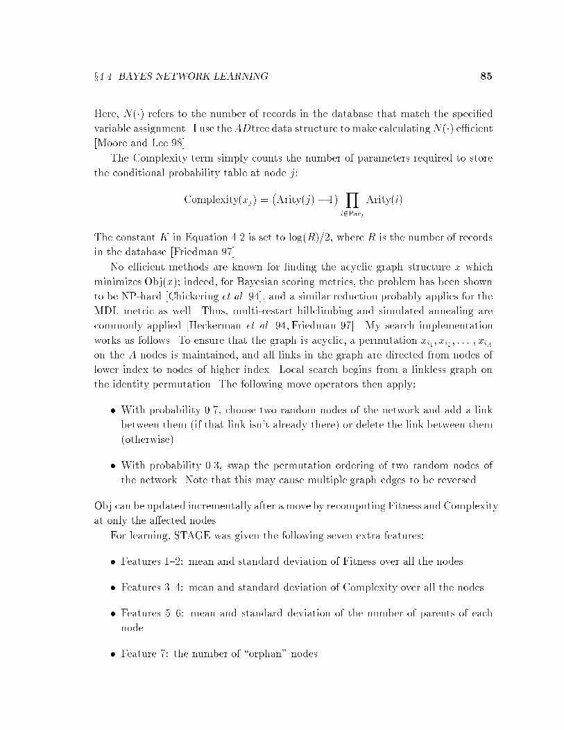
x4.4 BAYES NETWORK LEARNING 85
Here, N(�) refers to the number of records in the database that match the speci�ed
variable assignment. I use theADtree data structure to make calculatingN(�) e�cient
[Moore and Lee 98].
The Complexity term simply counts the number of parameters required to store
the conditional probability table at node j:
Complexity(xj) =�Arity(j)� 1
� Yi2Parj
Arity(i)
The constant K in Equation 4.2 is set to log(R)=2, where R is the number of records
in the database [Friedman 97].
No e�cient methods are known for �nding the acyclic graph structure x which
minimizes Obj(x); indeed, for Bayesian scoring metrics, the problem has been shown
to be NP-hard [Chickering et al. 94], and a similar reduction probably applies for the
MDL metric as well. Thus, multi-restart hillclimbing and simulated annealing are
commonly applied [Heckerman et al. 94, Friedman 97]. My search implementation
works as follows. To ensure that the graph is acyclic, a permutation xi1; xi2; : : : ; xiAon the A nodes is maintained, and all links in the graph are directed from nodes of
lower index to nodes of higher index. Local search begins from a linkless graph on
the identity permutation. The following move operators then apply:
� With probability 0.7, choose two random nodes of the network and add a link
between them (if that link isn't already there) or delete the link between them
(otherwise).
� With probability 0.3, swap the permutation ordering of two random nodes of
the network. Note that this may cause multiple graph edges to be reversed.
Obj can be updated incrementally after a move by recomputing Fitness and Complexity
at only the a�ected nodes.
For learning, STAGE was given the following seven extra features:
� Features 1{2: mean and standard deviation of Fitness over all the nodes
� Features 3{4: mean and standard deviation of Complexity over all the nodes
� Features 5{6: mean and standard deviation of the number of parents of each
node
� Feature 7: the number of \orphan" nodes
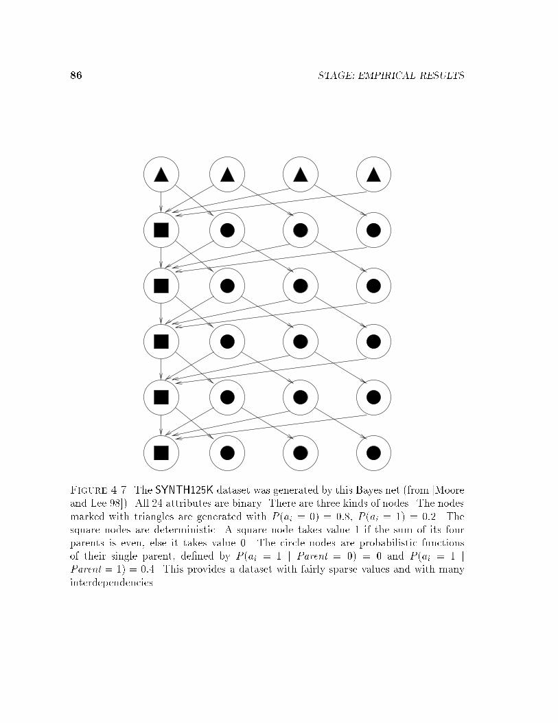
86 STAGE: EMPIRICAL RESULTS
Figure 4.7. The SYNTH125K dataset was generated by this Bayes net (from [Mooreand Lee 98]). All 24 attributes are binary. There are three kinds of nodes. The nodesmarked with triangles are generated with P (ai = 0) = 0:8, P (ai = 1) = 0:2. Thesquare nodes are deterministic. A square node takes value 1 if the sum of its fourparents is even, else it takes value 0. The circle nodes are probabilistic functionsof their single parent, de�ned by P (ai = 1 j Parent = 0) = 0 and P (ai = 1 jParent = 1) = 0:4. This provides a dataset with fairly sparse values and with manyinterdependencies.

x4.4 BAYES NETWORK LEARNING 87
Figure 4.8. A network structure learned by a sample run of STAGE from theSYNTH125K dataset. Its Obj score is 719074. By comparison, the actual networkthat was used to generate the data (shown earlier in Figure 4.7) scores 718641. Onlytwo edges from the generator net are missing from the learned net. The learned netincludes 17 edges not in the generator net (shown as curved arcs).

88 STAGE: EMPIRICAL RESULTS
I applied STAGE to three datasets: MPG, a small dataset consisting of 392 records
of 10 attributes each; ADULT2, a large real-world dataset consisting of 30,162 records
of 15 attributes each; and SYNTH125K, a synthetic dataset consisting of 125,000
records of 24 attributes each. The synthetic dataset was generated by sampling from
the Bayes net depicted in Figure 4.7. A perfect reconstruction of that net would
receive a score of Obj(x) = 718641. For further details of the other datasets, please
see Appendix C.3.
The STAGE parameters shown in Table 4.6 were used in all domains. Figures 4.9{
4.11 and Table 4.7 contrast the performance of hillclimbing (HC), simulated annealing
(SA) and STAGE. For reference, the table also gives the score of the \linkless" Bayes
net|corresponding to the simplestmodel of the data, that all attributes are generated
independently.
Parameter Setting
� stochastic hillclimbing, patience=200ObjBound 0features 7 (Fitness �; �; Complexity �; �;#Parents �; �;#Orphans)�tter quadratic regressionPat 200TotEvals 100,000
Table 4.6. Summary of STAGE parameters for Bayes net results
Instance Algorithm Performance (100 runs each) � moves
mean best worst time accepted
MPG HC 3563.4� 0.3 3561.3 3567.4 35s 5%(linkless score SA 3568.2� 0.9 3561.3 3595.5 47s 30%= 5339.4) STAGE 3564.1� 0.4 3561.3 3569.5 48s 2%ADULT2 HC 440567� 52 439912 441171 239s 6%(linkless score SA 440924� 134 439551 444094 446s 28%= 554090) STAGE 440432� 57 439773 441052 351s 6%SYNTH125K HC 748201�1714 725364 766325 151s 10%(linkless score SA 726882�1405 718904 754002 142s 29%= 1,594,498) STAGE 730399�1852 718804 782531 156s 4%
Table 4.7. Bayes net structure-�nding results
On SYNTH125K, the largest dataset, simulated annealing and STAGE both im-
prove signi�cantly over multi-restart hillclimbing, usually attaining a score within 2%
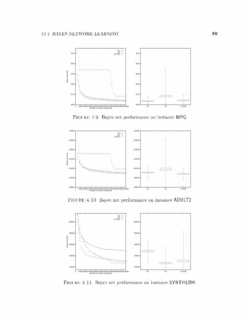
x4.4 BAYES NETWORK LEARNING 89
3560
3570
3580
3590
3600
3610
0 10000 20000 30000 40000 50000 60000 70000 80000 90000100000
Bay
es n
et s
core
Number of moves considered
HCSA
STAGE
3560
3570
3580
3590
3600
3610
HC SA STAGE
Figure 4.9. Bayes net performance on instance MPG
439000
440000
441000
442000
443000
444000
445000
0 10000 20000 30000 40000 50000 60000 70000 80000 90000100000
Bay
es n
et s
core
Number of moves considered
HCSA
STAGE
439000
440000
441000
442000
443000
444000
445000
HC SA STAGE
Figure 4.10. Bayes net performance on instance ADULT2
720000
740000
760000
780000
800000
0 10000 20000 30000 40000 50000 60000 70000 80000 90000100000
Bay
es n
et s
core
Number of moves considered
HCSA
STAGE
720000
740000
760000
780000
800000
HC SA STAGE
Figure 4.11. Bayes net performance on instance SYNTH125K

90 STAGE: EMPIRICAL RESULTS
of that of the Bayes net that generated the data, and on some runs coming within
0.04%. A good solution found by STAGE is drawn in Figure 4.8. Simulated an-
nealing slightly outperforms STAGE on average (however, Section 6.1.5 describes an
extension which improves STAGE's performance on SYNTH125K). On the MPG and
ADULT2 datasets, HC and STAGE performed comparably, while SA did slightly less
well on average. SA's odd-looking performance curves deserve further explanation. It
turns out that they are a side e�ect of the large scale of the objective function: when
single moves incur large changes in Obj, the adaptive annealing schedule (refer to Ap-
pendix B) takes longer to raise the temperature to a suitably high initial level, which
means that the initial part of SA's trajectory is e�ectively performing hillclimbing.
During this phase SA can �nd quite a good solution, especially in the real datasets
(MPG and ADULT2), for which the initial state (the linkless graph) is a good starting
point for hillclimbing. The good early solutions, then, are never bettered until the
temperature decreases late in the schedule; hence the best-so-far curve is at for most
of each run.
All algorithms require comparable amounts of total run time, except on the
ADULT2 task where SA and STAGE both run slower than HC. On that task, the dif-
ference in run times appears to be caused by the types of graph structures explored
during search; SA and STAGE spend greater e�ort exploring more complex net-
works with more connections, at which the objective function evaluates more slowly.
STAGE's computational overhead for learning is insigni�cant.
In sum, STAGE's performance on the Bayes net learning task was less dominant
than on the bin-packing and channel routing tasks, but it was still more consistently
best or nearly best than either HC or SA on the three benchmark instances attempted.
4.5 Radiotherapy Treatment Planning
Radiation therapy is a method of treating tumors [Censor et al. 88]. As illustrated
in Figure 4.12, a linear accelerator that produces a radioactive beam is mounted on
a rotating gantry, and the patient is placed so that the tumor is at the center of the
beam's rotation. Depending on the exact equipment being used, the beam can be
shaped in various ways as it rotates around the patient. A radiotherapy treatment
plan speci�es the beam's shape and intensity at a �xed number of source angles.
A map of the relevant part of the patient's body, with the tumor and all im-
portant structures labelled, is available. Also known are reasonably good clinical
forward models for calculating, from a treatment plan, the distribution of radiation
that will be delivered to the patient's tissues. The optimization task, then, is the
following \inverse problem": given the map and the forward model, produce a treat-

x4.5 RADIOTHERAPY TREATMENT PLANNING 91
Figure 4.12. Radiotherapy treatment planning (from [Censor et al. 88])
ment plan that meets target radiation doses for the tumor while minimizing damage
to sensitive nearby structures. In current practice, simulated annealing and/or linear
programming are often used for this problem [Webb 91,Webb 94].
Figure 4.13 illustrates a simpli�ed planar instance of the radiotherapy problem.
The instance consists of an irregularly shaped tumor and four sensitive structures: the
eyes, the brainstem, and the rest of the head. A treatment for this instance consists of
a plan to turn the accelerator beam either on or o� at each of 100 beam angles evenly
spaced within [�3�4; 3�
4]. Given a treatment plan, the objective function is calculated
by summing ten terms: an overdose penalty and an underdose penalty for each of the
�ve structures. For details of the penalty terms, please refer to Appendix C.4.
I applied hillclimbing (HC), simulated annealing (SA), and STAGE to this domain.
Objective function evaluations are computationally expensive here, so my experiments
considered only 10,000 moves per run. The features provided to STAGE consisted of
the ten subcomponents of the objective function. STAGE's parameter settings are
given in Table 4.8.
Results of 200 runs of each algorithm are shown in Figure 4.14 and Table 4.9. All
performed comparably, but STAGE's solutions were best on average. Note, however,
that the very best solution over all 600 runs was found by a hillclimbing run. The
objective function computation dominates the running time; STAGE's overhead for
learning is relatively insigni�cant.

92 STAGE: EMPIRICAL RESULTS
EYE1 EYE2
BRAINSTEM TUMOR
Figure 4.13. Radiotherapy instance 5E
Parameter Setting
� stochastic hillclimbing, patience=200ObjBound 0features 10 (overdose penalty and underdose penalty for each organ)�tter quadratic regressionPat 200TotEvals 10,000
Table 4.8. Summary of STAGE parameters for radiotherapy results
Instance Algorithm Performance (200 runs each) � moves
mean best worst time accepted
5E HC 18.822�0.030 18.003 19.294 550s 5.5%SA 18.817�0.043 18.376 19.395 460s 29%STAGE 18.721�0.029 18.294 19.155 530s 4.9%
Table 4.9. Radiotherapy results
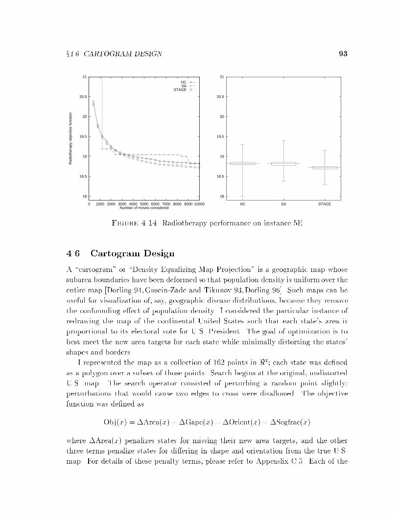
x4.6 CARTOGRAM DESIGN 93
18
18.5
19
19.5
20
20.5
21
0 1000 2000 3000 4000 5000 6000 7000 8000 9000 10000
Rad
ioth
erap
y ob
ject
ive
func
tion
Number of moves considered
HCSA
STAGE
18
18.5
19
19.5
20
20.5
21
HC SA STAGE
Figure 4.14. Radiotherapy performance on instance 5E
4.6 Cartogram Design
A \cartogram" or \Density Equalizing Map Projection" is a geographic map whose
subarea boundaries have been deformed so that population density is uniform over the
entire map [Dorling 94,Gusein-Zade and Tikunov 93,Dorling 96]. Such maps can be
useful for visualization of, say, geographic disease distributions, because they remove
the confounding e�ect of population density. I considered the particular instance of
redrawing the map of the continental United States such that each state's area is
proportional to its electoral vote for U.S. President. The goal of optimization is to
best meet the new area targets for each state while minimally distorting the states'
shapes and borders.
I represented the map as a collection of 162 points in <2; each state was de�ned
as a polygon over a subset of those points. Search begins at the original, undistorted
U.S. map. The search operator consisted of perturbing a random point slightly;
perturbations that would cause two edges to cross were disallowed. The objective
function was de�ned as
Obj(x) = �Area(x) + �Gape(x) + �Orient(x) + �Segfrac(x)
where �Area(x) penalizes states for missing their new area targets, and the other
three terms penalize states for di�ering in shape and orientation from the true U.S.
map. For details of these penalty terms, please refer to Appendix C.5. Each of the

94 STAGE: EMPIRICAL RESULTS
CA
OR
WA
NV
AZ
UT
IDMT
WY
CO
NM
TX
OK
KS
NE
SD
NDMN
IA
MO
AR
LAMS AL GA
FL
SCTN NCKY
VAWV
MDDENJCTRIMA
MENHVT
NY
PAOHINIL
WIMI
DC
CA
ORWA
NV
AZ
UT
IDMT
WY
CO
NM
TXOK
KS
NESDND MN
IA
MO
AR
LAMS AL GA
FL
SC
TNNC
KY VAWV MD
DE
NJ
CTRIMA
ME
NHVT
NY
PAOHINIL
WIMI
DC
L2L1
OCEAN
CA
ORWA
NV
AZ
UT
IDMTWY
CO
NM
TX
OK
KS
NESDND
MN
IA
MO
AR
LA
MS AL GA
FL
SCTN NCKY
VAWV MDDE
NJ
CTRI
MA
MENHVT
NY
PAOH
INIL
WI MI
DC
Figure 4.15. Cartograms of the continental U.S. Each state's target area is propor-tional to its electoral vote for U.S. President. The undistorted U.S. map (top left) haszero penalty for state shapes and orientations but a large penalty for state areas, soObj(x) = 525:7. Hillclimbing produces solutions like the one shown at top right, forwhich Obj(x) = 0:115: The third cartogram, found by STAGE, has Obj(x) = 0:043:

x4.7 BOOLEAN SATISFIABILITY 95
feature values can be updated incrementally when a single vertex is moved, so local
search can be applied to optimize Obj(x) quite e�ciently.
For STAGE, I represented each con�guration by four features|namely, the four
subcomponents of Obj. Learning a new evaluation function with quadratic regression
over these features, STAGE produced a signi�cant improvement over hillclimbing, but
was outperformed by simulated annealing. Table 4.10 shows STAGE's parameters,
and Table 4.11 and Figure 4.16 show the results. Later, in Sections 5.2.1{5.2.4, I
report the results of further experiments on the cartogram domain using varying
feature sets and function approximators.
Parameter Setting
� stochastic hillclimbing, patience=200ObjBound 0features 4 (subcomponents of Obj)�tter quadratic regressionPat 200TotEvals 1,000,000
Table 4.10. Summary of STAGE parameters for cartogram results
Instance Algorithm Performance (100 runs each) � moves
mean best worst time accepted
US49 HC 0.174�0.002 0.152 0.195 190s 14%SA 0.037�0.003 0.031 0.170 130s 32%STAGE 0.056�0.003 0.038 0.132 172s 7%
Table 4.11. Cartogram results
4.7 Boolean Satis�ability
4.7.1 WALKSAT
Finding a variable assignment that satis�es a large Boolean expression is a fundamental|
indeed, the original|NP-complete problem [Garey and Johnson 79]. In recent years,
surprisingly di�cult formulas have been solved by WALKSAT [Selman et al. 96], a
simple local search method. WALKSAT, given a formula expressed in CNF (a con-
junction of disjunctive clauses), conducts a random walk in assignment space that is

96 STAGE: EMPIRICAL RESULTS
0
0.1
0.2
0.3
0.4
0.5
200000 400000 600000 800000 1e+06
Map
err
or fu
nctio
n
Number of moves considered
HCSA
STAGE
0
0.1
0.2
0.3
0.4
0.5
HC SA STAGE
Figure 4.16. Cartogram performance on instance US49
biased toward minimizing
Obj(x) = # of clauses unsatis�ed by assignment x.
When Obj(x) = 0, all clauses are satis�ed and the formula is solved.
WALKSAT searches as follows. On each step, it �rst selects an unsatis�ed clause
at random; it will satisfy that clause by ipping one variable within it. To decide
which one, it �rst evaluates how much overall improvement to Obj would result from
ipping each variable. If the best such improvement is positive, it greedily ips a
variable that attains that improvement. Otherwise, it ips a variable which worsens
Obj: with probability (1-noise), a variable which harms Obj the least, and with
probability noise, a variable at random from the clause. The best setting of noise is
problem-dependent [McAllester et al. 97].
WALKSAT is so e�ective that it has rendered nearly obsolete an archive of
several hundred benchmark problems collected for a 1993 DIMACS Challenge on
satis�ability [Selman et al. 96]. Within that archive, only the \32-bit parity func-
tion learning" instances (nefariously constructed by Crawford, Kearns, Schapire, and
Hirsh [Crawford 93]) are known to be solvable in principle, yet not solvable byWALK-
SAT. The development of an algorithm to solve these 32-bit parity instances has been
listed as one of ten outstanding challenges for research in propositional reasoning and
search [Selman et al. 97]. Most of my experiments in the satis�ability domain have
focused on the �rst such instance in the archive, par32-1.cnf, a formula consisting of

x4.7 BOOLEAN SATISFIABILITY 97
10277 clauses on 3176 variables. After presenting extensive results on this instance,
I will report additional results on the four other benchmark instances in the par32
family.
4.7.2 Experimental Setup
WALKSAT is generally run in a random multi-restart regime: after every cuto�
search steps, where cuto� is another parameter of the algorithm, it resets the search to
a random new assignment. Can STAGE, by observing WALKSAT trajectories, learn
a smarter restart policy? Certainly, a variety of additional state features potentially
useful for STAGE's learning are readily available in this domain. I used the following
set of �ve simple features:
� proportion of clauses currently unsatis�ed (/ Obj(x))
� proportion of clauses satis�ed by exactly 1 variable
� proportion of clauses satis�ed by exactly 2 variables
� proportion of variables that would break a clause if ipped
� proportion of variables set to their \naive" setting4
All of these features can be computed incrementally in O(1) time after any variable
is ipped.
For comparison, I evaluated the performance of the following algorithms, allowing
each a total of 108 bit ips per run:
� (HC): random multi-start hillclimbing, patience = 104, accepting equi-cost
moves. Candidate moves are generated using the same bit- ip distribution
as WALKSAT, but moves that increase the number of unsatis�ed clauses are
rejected.
� (S/HC): STAGE applied to � = HC. Quadratic regression is used to predict
hillclimbing outcomes from the �ve features above. For STAGE's second phase
(stochastic hillclimbing on V �), the patience is set to 1000, and candidate bits
to ip are chosen uniformly at random, not with the WALKSAT distribution.
4Given a CNF formula F , the naive setting of variable xi is de�ned to be 0 if :xi appears inmore clauses of F than xi, or 1 if xi appears in more clauses than :xi.
98 STAGE: EMPIRICAL RESULTS
� (W): WALKSAT, noise = 0, cuto� = 106. These parameter settings were hand-
tuned for best performance over the range noise 2 f0; 0:05; 0:1; 0:15; : : : ; 0:5g,
cuto� 2 f103; 104; 105; 106; 107; 108g. Note that the chosen cuto� level of 106
means that WALKSAT performs exactly 100 random restarts per run.
� (S/W): STAGE applied to � = WALKSAT. This combination raises some
technical issues involving WALKSAT's termination criterion, as I explain below.
Theoretically, as discussed in Section 3.4.1, STAGE can learn from any procedure
� that is proper (guaranteed to terminate) and Markovian. WALKSAT's normal ter-
mination mechanism, cutting o� after a pre-speci�ed number of steps, is not Marko-
vian: it depends on an extraneous counter variable, not just the current assignment.
To apply STAGE to � = WALKSAT, I tried three modi�ed termination criteria:
� (S/W1): use STAGE's normal patience-based mechanism for cutting o� each
WALKSAT trajectory, just as I do for hillclimbing. Since WALKSAT is non-
monotonic, this mechanism also violates the Markov property: the probability
of cutting o� at state x depends not just on x but also on an extraneous counter
variable and the best Obj value seen previously. However, this is easily corrected
by the following adjustment.
� (S/W2): use patience-based cuto�s, but train the function approximator on only
the best-so-far states of each sample WALKSAT trajectory. By Proposition 2
(presented on page 62, proven in Appendix A.1), this subsequence of states
constitutes a sample trajectory from a higher-level search procedure which is
proper, strictly monotonic, and Markovian, so V � is well-de�ned.
� (S/W3): cut o� WALKSAT's trajectory with a �xed probability � > 0 after
every ip. This approach results in a proper Markovian trajectory, so V � is
again well-de�ned. A possible drawback to this approach is that termination
may randomly occur during a fruitful part of the search trajectory.
For (S/W1), I hand-tuned WALKSAT's noise and patience parameters over the same
ranges I used for tuning Experiment (W). Here, I found best performance at noise =
0:25 (more random actions) and patience = 104 (more frequent restarting). Without
further tuning, I set patience = 104 in (S/W2), � = 10�4 in (S/W3), and noise = 0:25
in both. The parameters for STAGE's second phase, hillclimbing on V �, were set as
in Experiment (S/HC) above.
Serendipitously, I discovered that introducing an additional WALKSAT param-
eter could improve STAGE's performance. The new parameter, call it �w, has the
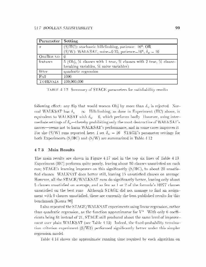
x4.7 BOOLEAN SATISFIABILITY 99
Parameter Setting
� (S/HC): stochastic hillclimbing, patience=104; OR(S/W): WALKSAT, noise=0.25, patience=104, �w = 10
ObjBound 0features 5 (Obj, % clauses with 1 true, % clauses with 2 true, % clause-
breaking variables, % naive variables)�tter quadratic regressionPat 1000TotEvals 100,000,000
Table 4.12. Summary of STAGE parameters for satis�ability results
following e�ect: any ip that would worsen Obj by more than �w is rejected. Nor-
mal WALKSAT has �w = 1. Hillclimbing, as done in Experiment (HC) above, is
equivalent to WALKSAT with �w = 0, which performs badly. However, using inter-
mediate settings of �w|thereby prohibiting only the most destructive of WALKSAT's
moves|seems not to harm WALKSAT's performance, and in some cases improves it.
For the (S/W) runs reported here, I set �w = 10. STAGE's parameter settings for
both Experiments (S/HC) and (S/W) are summarized in Table 4.12.
4.7.3 Main Results
The main results are shown in Figure 4.17 and in the top six lines of Table 4.13.
Experiment (HC) performs quite poorly, leaving about 50 clauses unsatis�ed on each
run; STAGE's learning improves on this signi�cantly (S/HC), to about 20 unsatis-
�ed clauses. WALKSAT does better still, leaving 15 unsatis�ed clauses on average.
However, all the STAGE/WALKSAT runs do signi�cantly better, leaving only about
5 clauses unsatis�ed on average, and as few as 1 or 2 of the formula's 10277 clauses
unsatis�ed on the best runs. Although STAGE did not manage to �nd an assign-
ment with 0 clauses unsatis�ed, these are currently the best published results for this
benchmark [Kautz 98].
I also repeated the STAGE/WALKSAT experiments using linear regression, rather
than quadratic regression, as the function approximator for V �. With only 6 coe�-
cients being �t instead of 21, STAGE still produced about the same level of improve-
ment over plain WALKSAT (see Table 4.13). Indeed, the �xed-probability termina-
tion criterion experiment (S/W3) performed signi�cantly better under this simpler
regression model.
Table 4.14 shows the approximate running time required by each algorithm on

100 STAGE: EMPIRICAL RESULTS
Instance Algorithm Performance (N runs each)mean best worst
par32-1.cnf HC 48.03�0.59 40 54(N = 100) S/HC (STAGE, � = hillclimbing) 21.64�0.77 11 31
W (WALKSAT) 15.22�0.35 9 19S/W1 (STAGE, � = WALKSAT) 5.36�0.33 1 9S/W2 5.04�0.27 2 8S/W3 5.60�0.29 2 9S/W1+linear 5.27�0.37 2 14S/W2+linear 6.21�0.30 2 10S/W3+linear 4.43�0.28 2 8
par32-2.cnf W 15.40�0.57 13 18(N = 25) S/W3+linear 4.32�0.48 2 7par32-3.cnf W 15.84�0.45 14 18(N = 25) S/W3+linear 4.32�0.53 2 7par32-4.cnf W 15.28�0.46 13 17(N = 25) S/W3+linear 4.63�0.60 2 7par32-5.cnf W 15.48�0.61 11 18(N = 25) S/W3+linear 4.76�0.63 2 9
Table 4.13. Satis�ability results on the 32-bit parity benchmarks
0
10
20
30
40
50
60
2e+07 4e+07 6e+07 8e+07 1e+08
Uns
atis
fied
clau
ses
Number of moves considered
HCS/HC
WS/W1S/W2S/W3
0
10
20
30
40
50
60
HC S/HC W S/W1 S/W2 S/W3
Figure 4.17. Satis�ability: main results on instance par32-1.cnf
x4.7 BOOLEAN SATISFIABILITY 101
instance par32-1.cnf. In this domain, STAGE takes about twice as long to complete
as WALKSAT; for that matter, so does hillclimbing (HC). By pro�ling the executions,
I identi�ed three sources of the disparity. First, WALKSAT saves time by accepting
all of the 108 proposed bit ips. Every time HC or STAGE rejects a move, it must
un ip the modi�ed bit and re-update the counts of violated clauses, so rejecting a
move takes twice as long as accepting a move. Second, for all the STAGE runs other
than S/W2, signi�cant time is spent in memory management for storing WALKSAT
trajectories. These trajectories often consist of tens of thousands of states, and my
implementation is not optimized to handle such long trajectories e�ciently. Since
the S/W2 runs train on only the best-so-far states, they have much less data to store
and do not pay this penalty. Finally, the function approximation (computing the
coe�cients of ~V � by least-squares regression) adds about 3% additional overhead to
STAGE's running time.
Table 4.14 also reveals that the S/W3+linear run accepts fully 97% of its moves.
This simply indicates that it is spending the bulk of its e�ort in the WALKSAT stage
of search (during which 100% of moves are accepted), and relatively little time on the
stage of hillclimbing on ~V �. A closer look shows that this happens because the linear
approximation is quite inaccurate, with an RMS error of 9.5 on its training set, and
STAGE's ObjBound parameter cuts o� hillclimbing as soon as the predicted ~V �(x)
falls below zero|typically after only a few hundred moves on each iteration. Though
these runs reject fewer moves than their S/W3+quadratic counterparts, their extra
WALKSAT runs mean extra memory management for trajectory storage, so their
running time is not signi�cantly lessened.
Despite STAGE's overhead in this domain, it is clear from the plot of Figure 4.17
that even if running times were equalized by halving STAGE's allotted number of
moves, STAGE's performance would still signi�cantly exceed pure WALKSAT's.
4.7.4 Follow-up Experiments
I conducted three additional follow-up experiments. First, I compared pure WALK-
SAT with STAGE/WALKSAT on the other four 32-bit parity instances from the
DIMACS archive. The results, shown in Table 4.13, corroborate the results on par32-
1: STAGE consistently leaves 2=3 fewer unsatis�ed clauses than WALKSAT on these
problems.
Second, I studied each of the WALKSAT parameter di�erences between Exper-
iments (W) and (S/W3) in isolation. Speci�cally, I ran eight head-to-head exper-
imental comparisons of WALKSAT and STAGE/WALKSAT with the WALKSAT
parameters �xed to be the same in both algorithms. The eight experiments corre-
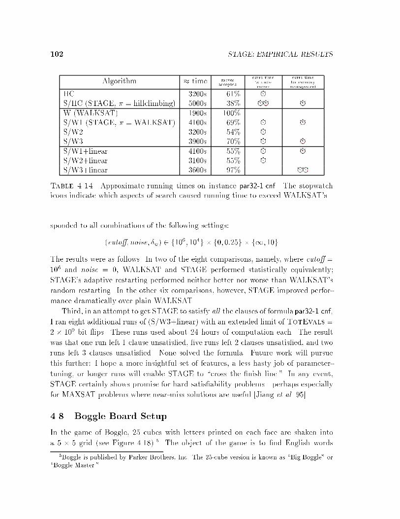
102 STAGE: EMPIRICAL RESULTS
Algorithm � time movesaccepted
extra timeto undomoves
extra timefor memorymanagement
HC 3200s 61%S/HC (STAGE, � = hillclimbing) 5000s 38%W (WALKSAT) 1900s 100%S/W1 (STAGE, � = WALKSAT) 4100s 69%S/W2 3200s 54%S/W3 3900s 70%S/W1+linear 4100s 55%S/W2+linear 3100s 55%S/W3+linear 3600s 97%
Table 4.14. Approximate running times on instance par32-1.cnf. The stopwatchicons indicate which aspects of search caused running time to exceed WALKSAT's.
sponded to all combinations of the following settings:
(cuto�;noise; �w) 2 f106; 104g � f0; 0:25g � f1; 10g
The results were as follows. In two of the eight comparisons, namely, where cuto� =
106 and noise = 0, WALKSAT and STAGE performed statistically equivalently;
STAGE's adaptive restarting performed neither better nor worse than WALKSAT's
random restarting. In the other six comparisons, however, STAGE improved perfor-
mance dramatically over plain WALKSAT.
Third, in an attempt to get STAGE to satisfy all the clauses of formula par32-1.cnf,
I ran eight additional runs of (S/W3+linear) with an extended limit of TotEvals =
2 � 109 bit ips. These runs used about 24 hours of computation each. The result
was that one run left 1 clause unsatis�ed, �ve runs left 2 clauses unsatis�ed, and two
runs left 3 clauses unsatis�ed. None solved the formula. Future work will pursue
this further: I hope a more insightful set of features, a less hasty job of parameter-
tuning, or longer runs will enable STAGE to \cross the �nish line." In any event,
STAGE certainly shows promise for hard satis�ability problems|perhaps especially
for MAXSAT problems where near-miss solutions are useful [Jiang et al. 95].
4.8 Boggle Board Setup
In the game of Boggle, 25 cubes with letters printed on each face are shaken into
a 5 � 5 grid (see Figure 4.18).5 The object of the game is to �nd English words
5Boggle is published by Parker Brothers, Inc. The 25-cube version is known as \Big Boggle" or\Boggle Master."
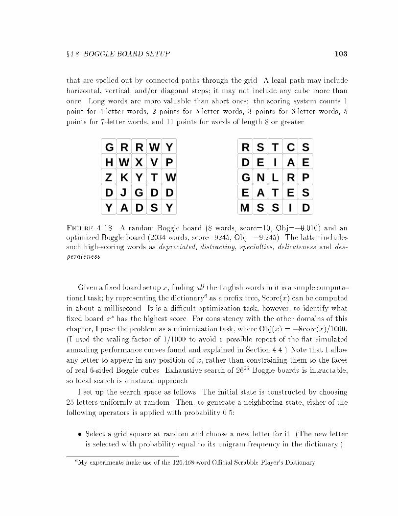
x4.8 BOGGLE BOARD SETUP 103
that are spelled out by connected paths through the grid. A legal path may include
horizontal, vertical, and/or diagonal steps; it may not include any cube more than
once. Long words are more valuable than short ones: the scoring system counts 1
point for 4-letter words, 2 points for 5-letter words, 3 points for 6-letter words, 5
points for 7-letter words, and 11 points for words of length 8 or greater.
G R YH V PZ K Y WD D D
A D Y
RW X
W
T
SYJ G
R S T C SD E A EG N L R PE A T E S
S S D
I
IM
Figure 4.18. A random Boggle board (8 words, score=10, Obj=�0:010) and anoptimized Boggle board (2034 words, score=9245, Obj=�9:245). The latter includessuch high-scoring words as depreciated, distracting, specialties, delicateness and des-perateness.
Given a �xed board setup x, �nding all the English words in it is a simple computa-
tional task; by representing the dictionary6 as a pre�x tree, Score(x) can be computed
in about a millisecond. It is a di�cult optimization task, however, to identify what
�xed board x� has the highest score. For consistency with the other domains of this
chapter, I pose the problem as a minimization task, where Obj(x) = �Score(x)=1000:
(I used the scaling factor of 1=1000 to avoid a possible repeat of the at simulated
annealing performance curves found and explained in Section 4.4.) Note that I allow
any letter to appear in any position of x, rather than constraining them to the faces
of real 6-sided Boggle cubes. Exhaustive search of 2625 Boggle boards is intractable,
so local search is a natural approach.
I set up the search space as follows. The initial state is constructed by choosing
25 letters uniformly at random. Then, to generate a neighboring state, either of the
following operators is applied with probability 0.5:
� Select a grid square at random and choose a new letter for it. (The new letter
is selected with probability equal to its unigram frequency in the dictionary.)
6My experiments make use of the 126,468-word O�cial Scrabble Player's Dictionary.
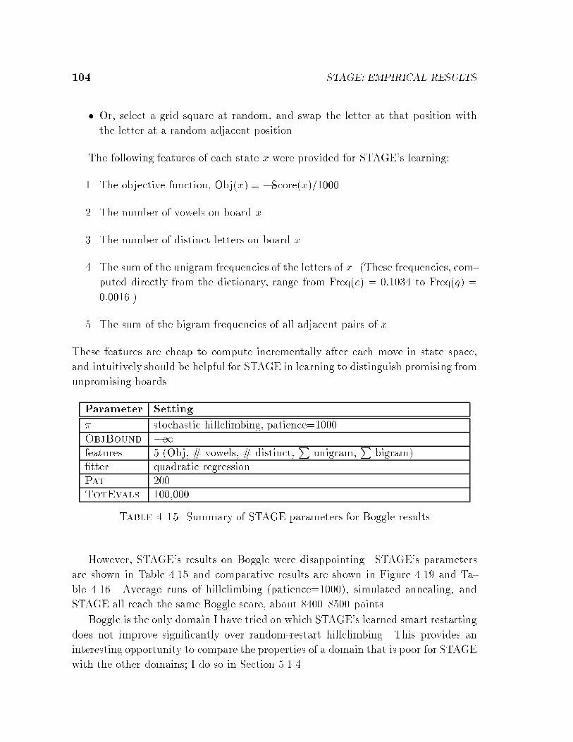
104 STAGE: EMPIRICAL RESULTS
� Or, select a grid square at random, and swap the letter at that position with
the letter at a random adjacent position.
The following features of each state x were provided for STAGE's learning:
1. The objective function, Obj(x) = �Score(x)=1000.
2. The number of vowels on board x.
3. The number of distinct letters on board x.
4. The sum of the unigram frequencies of the letters of x. (These frequencies, com-
puted directly from the dictionary, range from Freq(e) = 0:1034 to Freq(q) =
0:0016.)
5. The sum of the bigram frequencies of all adjacent pairs of x.
These features are cheap to compute incrementally after each move in state space,
and intuitively should be helpful for STAGE in learning to distinguish promising from
unpromising boards.
Parameter Setting
� stochastic hillclimbing, patience=1000ObjBound �1features 5 (Obj, # vowels, # distinct,
Punigram,
Pbigram)
�tter quadratic regressionPat 200TotEvals 100,000
Table 4.15. Summary of STAGE parameters for Boggle results
However, STAGE's results on Boggle were disappointing. STAGE's parameters
are shown in Table 4.15 and comparative results are shown in Figure 4.19 and Ta-
ble 4.16. Average runs of hillclimbing (patience=1000), simulated annealing, and
STAGE all reach the same Boggle score, about 8400{8500 points.
Boggle is the only domain I have tried on which STAGE's learned smart restarting
does not improve signi�cantly over random-restart hillclimbing. This provides an
interesting opportunity to compare the properties of a domain that is poor for STAGE
with the other domains; I do so in Section 5.1.4.

x4.8 BOGGLE BOARD SETUP 105
Instance Algorithm Performance (100 runs each) � moves
mean best worst time accepted
5 � 5 HC -8.413�0.066 -9.046 -7.473 2235s 2.4%SA -8.431�0.086 -9.272 -7.622 1720s 33%STAGE -8.480�0.077 -9.355 -7.570 2450s 1.3%
Table 4.16. Boggle results. The mean performances do not di�er signi�cantly fromone another.
-10
-9
-8
-7
-6
-5
-4
20000 40000 60000 80000 100000
- B
oggl
e sc
ore
(in th
ousa
nds)
Number of moves considered
HCSA
STAGE
-10
-9
-8
-7
-6
-5
-4
HC SA STAGE
Figure 4.19. Performance on the Boggle domain
106 STAGE: EMPIRICAL RESULTS
4.9 Discussion
This chapter has demonstrated that STAGE may be pro�tably applied to a wide
variety of global optimization problems. In addition to the domains reported here, an
algorithm closely related to STAGE has also been successfully applied to the \Dial-
a-Ride" problem, a variant of the Travelling Salesperson Problem, by Moll et al. [97].
Empirically, in both discrete domains (e.g., channel routing, Bayes net structure-
�nding, satis�ability) and continuous domains (e.g., cartogram design), STAGE is
able to learn from and improve upon the results of local search trajectories. In the
next chapter, I will probe more deeply into the reasons for STAGE's success.
107
Chapter 5
STAGE: Analysis
In the preceding chapter, I gave empirical evidence that STAGE is an e�ective
optimization technique for a wide variety of domains. In this chapter, I break down
the causes for that e�ectiveness. Does STAGE's power derive from its use of machine
learning, per its design? Or are incidental aspects of the way it organizes its search just
as responsible for STAGE's success? How robust is the algorithm to varying choices
of feature sets, function approximators, and other user-controllable parameters?
This chapter reports the results of a series of experiments that explore these
questions empirically. Most of the experiments are performed in the domains of VLSI
channel routing, as described in Section 4.3, and cartogram design, as described in
Section 4.6.
5.1 Explaining STAGE's Success
STAGE performs superbly on the channel routing domain, not only outperforming
hillclimbing as it was trained to do, but also �nding better solutions on average than
the best simulated annealing runs. How can we explain its success? There are at
least three possibilities:
Hypothesis A: STAGE works according to its design. Gathering data from a num-
ber of hillclimbing trajectories, it learns to predict the outcome of hillclimbing
starting from various state features, and it exploits these predictions to reach
improved local optima.
Hypothesis B: Since STAGE alternates between simple hillclimbing and another
policy, it simply bene�ts from having more random exploration. STAGE uses
hillclimbing on the learned ~V � as its secondary policy, but alternative policies
would do just as well.
Hypothesis C: The function approximator may simply be smoothing the objective
function, which helps eliminate local minima and plateaus.
In this section, I �rst describe experiments which reject the latter two hypotheses.
I then describe experiments giving further evidence for Hypothesis A, that STAGE
does indeed work as designed. Finally, I analyze an instance where STAGE failed.
108 STAGE: ANALYSIS
5.1.1 ~V � versus Other Secondary Policies
Hypothesis B attributes STAGE's success to its unusual regime of alternating between
hillclimbing and a secondary search policy. Perhaps any secondary policy which
perturbed the search away from its current local optimum would be just as e�ective
as STAGE's secondary policy of hillclimbing on the learned evaluation function ~V �.
To test this, I ran experiments with several alternative choices for STAGE's sec-
ondary policy:
Policy B0 (normal STAGE): Hillclimb on ~V �.
Policy B1: Perform a random walk of �xed length !. (I tried setting ! to 1, 3, 10,
and 40.)
Policy B2: Hillclimb on the inverse of ~V �. In other words, move stochastically to
a state which ~V � predicts to be the worst place from which to begin a search.
Policy B3: Hillclimb on a corrupted version of ~V �, trained by replacing every target
value in its training set with a random value.
Each of these policies was alternated with standard hillclimbing (patience=250), so
as to imitate STAGE's normal regime. Experiments B0, B2 and B3 approximated ~V �
using linear regression over the three channel routing features hw; p; Ui, each scaled to
the range [0; 1]. I ran each resulting algorithm 50 times on channel routing instance
YK4, limiting each run to TotEvals = 105 total moves considered. (Note that the
results of Section 4.3 were tabulated over longer runs of length TotEvals = 5 � 105.)
Instance Algorithm Performance (50 runs each)mean best worst
YK4 B0 (STAGE) 13.54�1.13 12 41B1 (! = 1) 16.94�0.23 15 19B1 (! = 3) 17.16�0.24 16 19B1 (! = 10) 19.12�0.27 17 21B1 (! = 40) 22.64�0.26 20 25B2 37.86�3.52 14 52B3 15.38�0.64 13 27
Table 5.1. Results of di�erent secondary policies on channel routing instance YK4.In each case, TotEvals = 105.
The results, given in Figure 5.1 and Table 5.1, show conclusively that the choice of
secondary policy does matter. STAGE's policy signi�cantly outperformed all others,
x5.1 EXPLAINING STAGE'S SUCCESS 109
10
15
20
25
30
35
40
45
50
0 10000 20000 30000 40000 50000 60000 70000 80000 90000100000
Are
a of
circ
uit l
ayou
t
Number of moves considered
STAGEB1(w= 1)B1(w= 3)B1(w=10)B1(w=40)
B2B3
10
15
20
25
30
35
40
45
50
STAGE B1(w=1) B1(w=3) B1(w=10)B1(w=40) B2 B3
Figure 5.1. Performance of di�erent secondary policies on channel routing instanceYK4
with 48 of its 50 runs producing a solution circuit of quality between 12 and 14.
(One outlier run did no better than 41; I analyze this in Section 5.1.3.) The random
walk policies (B1) were consistently inferior. Indeed, the pattern of the B1 results
shows clearly that performance degraded more and more as additional undirected
exploration was allowed. Experiment B2, in which the search was purposely led
against ~V � toward states judged unpromising, performed much worse than even the
random-walk policies. This provides further evidence that ~V � has learned useful
predictive information about the features.
Finally, Experiment B3 performed better than the random-walk policies, but still
signi�cantly worse than STAGE. Why did assigning random target values to the
training set for ~V � result in even moderately good performance? The answer is that
in this experiment, the linear regression model has only four coe�cients to �t, and
one of these (the coe�cient of the constant term) has no e�ect when ~V � is used as
an evaluation function to guide search. Thus, even choosing random values for the 3
meaningful coe�cients would sometimes lead search in the same useful direction as
the true V �. This analysis is supported by the plot of Figure 5.2. This plot compares
the successive local minima visited by a typical run of STAGE and a typical run of
Experiment B3. Clearly, STAGE learns a policy which keeps it in a high-quality part
of the space during most of its search, while B3 only occasionally \lucks into" a good
solution. Still, these results highlight the potential for an alternative algorithm to

110 STAGE: ANALYSIS
10
20
30
40
50
60
0 20000 40000 60000 80000 100000
Are
a of
circ
uit l
ayou
t
Number of moves considered
STAGEB3
Figure 5.2. Quality of local minima reached on each successive iteration of a STAGErun and a B3 run. Gaps in the STAGE plot correspond to iterations on which a restartoccurred.
STAGE, which works by optimizing the coe�cients of a ~V �-like function directly (see
Section 8.2.3).
The results of this series of experiments do not prove that hillclimbing on ~V �
is the only policy which can productively lead search away from a local minimum
and into the attracting basin of a potentially better local minimum. However, they
do at least demonstrate that not every secondary policy will be e�ective|and that
STAGE's learned policy is more e�ective than most.
5.1.2 ~V � versus Simple Smoothing
STAGE performs \predictive smoothing" of the original objective function Obj: the
function ~V � is a continuous mapping from the features of state x to the Obj value
that policy � is predicted to eventually reach from x. But perhaps, as suggested
by Hypothesis C above, the predictive aspect of STAGE's smoothing is irrelevant.
Perhaps STAGE's success could be replicated by simply smoothing Obj directly over
the feature space, which would eliminate the original objective function's local minima
and plateaus.
One aw of this hypothesis is immediately apparent: in channel routing as in most
of the other domains described in Chapter 4, the objective function value Obj(x) is

x5.1 EXPLAINING STAGE'S SUCCESS 111
provided to STAGE as one of the features of the input feature space. Therefore, any
function approximator could �t Obj perfectly over the feature space by simply copying
the Obj(x) feature from input to output. Clearly, this perfect \smoothing" of Obj
would not eliminate any local minima from Obj; STAGE would reduce to standard
multi-restart hillclimbing. Experiment C0, described below, empirically demonstrates
precisely this e�ect.
However, perhaps an imperfect smoothing of Obj would produce the hypothesized
good outcome. I performed the following series of experiments. For all experiments
except HC, the basic STAGE regime is unchanged; only the training set's target
values for the function approximator are modi�ed.
Experiment HC: Multi-restart hillclimbing, accepting equi-cost moves, patience =
500.
Experiment STAGE (same as Experiment B0): Normal STAGE, modelling V �(x)
by linear regression over the three features hw(x); p(x); U(x)i.
Experiment C0 (perfect \smoothing"): For each state in STAGE's training set,
represented by the features hw(x); p(x); U(x)i, train the function approximator
to model not V �(x) but the objective function Obj(x) = w(x). Here, the
function approximator can simply copy w(x) from input to output, so no real
smoothing occurs. Results are shown in Table 5.2 and Figure 5.3: as expected,
this policy performed similarly to multi-start hillclimbing.
Experiment C1: I eliminated the w feature from the training set, so the function
approximator had to model Obj(x) as a linear function of only hp(x); U(x)i.
The results were extremely poor. A closer look explained why. Recall that
Wong de�ned
U(x) =
w(x)Xi=1
ui(x)2
where ui(x) is the fraction of track i that is unoccupied [Wong et al. 88]. In
poor-quality solutions such as those visited at the beginning of a search, ui(x)
is close to 1 for each track, so U(x) � Obj(x). Thus, even a linear function
approximator can model Obj quite accurately by simply copying U(x) from
input to output. But this smoothed objective function, U(x), makes a terrible
evaluation function for optimization. Starting from a local optimum of Obj,
where no single move can reduce w(x) further, the only way a greedy search can
reduce U is to reduce the variance of the ui(x) values, that is, to distribute the
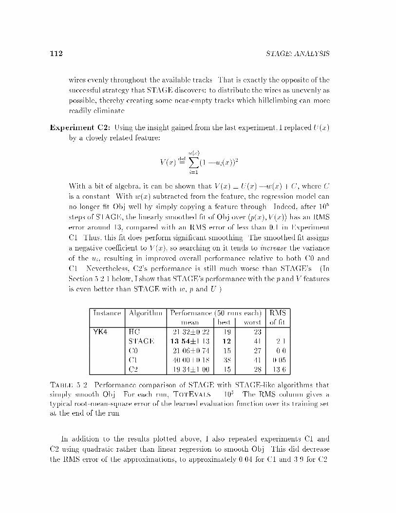
112 STAGE: ANALYSIS
wires evenly throughout the available tracks. That is exactly the opposite of the
successful strategy that STAGE discovers: to distribute the wires as unevenly as
possible, thereby creating some near-empty tracks which hillclimbing can more
readily eliminate.
Experiment C2: Using the insight gained from the last experiment, I replaced U(x)
by a closely related feature:
V (x)def=
w(x)Xi=1
(1 � ui(x))2
With a bit of algebra, it can be shown that V (x) � U(x)�w(x) +C, where C
is a constant. With w(x) subtracted from the feature, the regression model can
no longer �t Obj well by simply copying a feature through. Indeed, after 105
steps of STAGE, the linearly smoothed �t of Obj over hp(x); V (x)i has an RMS
error around 13, compared with an RMS error of less than 0:1 in Experiment
C1. Thus, this �t does perform signi�cant smoothing. The smoothed �t assigns
a negative coe�cient to V (x), so searching on it tends to increase the variance
of the ui, resulting in improved overall performance relative to both C0 and
C1. Nevertheless, C2's performance is still much worse than STAGE's. (In
Section 5.2.1 below, I show that STAGE's performance with the p and V features
is even better than STAGE with w, p and U .)
Instance Algorithm Performance (50 runs each) RMSmean best worst of �t
YK4 HC 21.32�0.22 19 23 |STAGE 13.54�1.13 12 41 2.1C0 21.06�0.74 15 27 0.0C1 40.00�0.18 38 41 0.05C2 19.34�1.00 15 28 13.6
Table 5.2. Performance comparison of STAGE with STAGE-like algorithms thatsimply smooth Obj. For each run, TotEvals = 105. The RMS column gives atypical root-mean-square error of the learned evaluation function over its training setat the end of the run.
In addition to the results plotted above, I also repeated experiments C1 and
C2 using quadratic rather than linear regression to smooth Obj. This did decrease
the RMS error of the approximations, to approximately 0.04 for C1 and 3.9 for C2.

x5.1 EXPLAINING STAGE'S SUCCESS 113
10
15
20
25
30
35
40
45
50
0 10000 20000 30000 40000 50000 60000 70000 80000 90000100000
Are
a of
circ
uit l
ayou
t
Number of moves considered
HCSTAGE
C0C1C2
10
15
20
25
30
35
40
45
50
HC STAGE C0 C1 C2
Figure 5.3. Performance on the experiments of Section 5.1.2
However, it did not improve optimization performance in either case. From this series
of experiments, I conclude that, at least for this problem, STAGE's success cannot
be attributed to simple smoothing of the objective function. STAGE's predictive
smoothing works signi�cantly better.
5.1.3 Learning Curves for Channel Routing
I have presented evidence that STAGE's secondary policy, searching on ~V �, is more
helpful to optimization than other reasonable policies based on randomness or smooth-
ing. This evidence contradicts Hypotheses B and C outlined on page 107. I now
examine STAGE's success on channel routing more closely, to support Hypothesis A:
that STAGE's leverage is indeed due to machine learning.
Figure 5.4 illustrates three short runs of STAGE on routing instance YK4. In each
row of the �gure, the left-hand graph illustrates the successive local minima visited
over the course of STAGE's run: a diamond symbol (}) marks a local minimum of
Obj, and a plus symbol (+) marks a local minimum of the learned evaluation function~V �. There is a gap in the plot each time STAGE resets search to the poor initial
state. Observe that the �rst two runs, (A) and (B), perform well, both attaining a
best solution quality of 12; whereas run (C) performs uncommonly poorly, with a
best solution quality of 34.
The right-hand graphs track the evolution of ~V � over the course of each run,
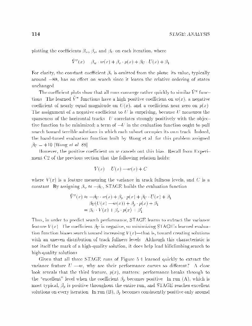
114 STAGE: ANALYSIS
plotting the coe�cients �w, �p, and �U on each iteration, where
~V �(x) = �w � w(x) + �p � p(x) + �U � U(x) + �1
For clarity, the constant coe�cient �1 is omitted from the plots: its value, typically
around �80, has no e�ect on search since it leaves the relative ordering of states
unchanged.
The coe�cient plots show that all runs converge rather quickly to similar ~V � func-
tions. The learned ~V � functions have a high positive coe�cient on w(x), a negative
coe�cient of nearly equal magnitude on U(x), and a coe�cient near zero on p(x).
The assignment of a negative coe�cient to U is surprising, because U measures the
sparseness of the horizontal tracks. U correlates strongly positively with the objec-
tive function to be minimized; a term of �U in the evaluation function ought to pull
search toward terrible solutions in which each subnet occupies its own track. Indeed,
the hand-tuned evaluation function built by Wong et al. for this problem assigned
�U = +10 [Wong et al. 88].
However, the positive coe�cient on w cancels out this bias. Recall from Experi-
ment C2 of the previous section that the following relation holds:
V (x) = U(x)� w(x) + C
where V (x) is a feature measuring the variance in track fullness levels, and C is a
constant. By assigning �w � ��U , STAGE builds the evaluation function
~V �(x) � ��U � w(x) + �p � p(x) + �U � U(x) + �1= �U(U(x)� w(x)) + �p � p(x) + �1= �U � V (x) + �p � p(x) + �01
Thus, in order to predict search performance, STAGE learns to extract the variance
feature V (x). The coe�cient �U is negative, so minimizing STAGE's learned evalua-
tion function biases search toward increasing V (x)|that is, toward creating solutions
with an uneven distribution of track fullness levels. Although this characteristic is
not itself the mark of a high-quality solution, it does help lead hillclimbing search to
high-quality solutions.
Given that all three STAGE runs of Figure 5.4 learned quickly to extract the
variance feature U � w, why are their performance curves so di�erent? A close
look reveals that the third feature, p(x), matters: performance breaks through to
the \excellent" level when the coe�cient �p becomes positive. In run (A), which is
most typical, �p is positive throughout the entire run, and STAGE reaches excellent
solutions on every iteration. In run (B), �p becomes consistently positive only around
x5.1 EXPLAINING STAGE'S SUCCESS 115
(A)
10
20
30
40
50
60
0 20000 40000 60000 80000 100000
Are
a of
circ
uit l
ayou
t
Number of moves considered
STAGE Trajectory (A)local optimum of Objlocal optimum of Vpi
-15
-10
-5
0
5
10
15
0 20000 40000 60000 80000 100000
Coe
ffici
ents
of l
earn
ed V
_pi f
unct
ion
Number of moves considered
coefficient on wcoefficient on pcoefficient on U
(B)
10
20
30
40
50
60
0 20000 40000 60000 80000 100000
Are
a of
circ
uit l
ayou
t
Number of moves considered
STAGE Trajectory (B)local optimum of Objlocal optimum of Vpi
-15
-10
-5
0
5
10
15
0 20000 40000 60000 80000 100000
Coe
ffici
ents
of l
earn
ed V
_pi f
unct
ion
Number of moves considered
coefficient on wcoefficient on pcoefficient on U
(C)
10
20
30
40
50
60
0 20000 40000 60000 80000 100000
Are
a of
circ
uit l
ayou
t
Number of moves considered
STAGE Trajectory (C)local optimum of Objlocal optimum of Vpi
-15
-10
-5
0
5
10
15
0 20000 40000 60000 80000 100000
Coe
ffici
ents
of l
earn
ed V
_pi f
unct
ion
Number of moves considered
coefficient on wcoefficient on pcoefficient on U
Figure 5.4. Three runs of STAGE on channel routing instance YK4. Left-handgraphs plot the Obj value reached at the end of each search trajectory within STAGE;right-hand graphs plot the evolution of the coe�cients of ~V �(x) over the run.

116 STAGE: ANALYSIS
(C)
10
20
30
40
50
60
0 100000 200000 300000 400000 500000
Are
a of
circ
uit l
ayou
t
Number of moves considered
STAGE Trajectory (C)local optimum of Objlocal optimum of Vpi
-15
-10
-5
0
5
10
15
0 100000 200000 300000 400000 500000
Coe
ffici
ents
of l
earn
ed V
_pi f
unct
ion
Number of moves considered
coefficient on wcoefficient on pcoefficient on U
Figure 5.5. Run (C) of Figure 5.4, extended to TotEvals = 500; 000.
move 60000, which corresponds to STAGE's breakthrough. Finally, in the outlier
run (C), �p remains negative throughout the �rst 100; 000 moves. However, it is slowly
increasing, and in fact, if the same run is allowed to extend to TotEvals = 500; 000,
then �p soon becomes positive and performance improves (see Figure 5.5). This run
reaches a solution quality of 12 after 145; 000 moves.
These runs illustrate that STAGE's convergence rate may depend on the particular
regions that STAGE happens to explore. In run (C), STAGE apparently becomes
\stuck" in a region of poor local optima until the �p coe�cient becomes positive,
triggering a random restart from which the learned ~V � can be e�ectively exploited.
This suggests that faster convergence may be attained by more frequent random
restarts; I investigate this in Section 5.2.4.
Despite the varying convergence rates, all the STAGE runs on instance YK4 do
eventually converge to an approximation of V � close to the following:
~V �(x) � 10 � w(x) + 0:5 � p(x) � 10 � U(x)� 80 (5.1)
The coe�cients on all three features are signi�cant. As discussed above, the compo-
nent 10(w(x) � U(x)) biases search toward solutions with an uneven distribution of
track fullness levels. As for p(x), recall from Section 4.3 that it provides a lower bound
on all solutions derived from x by future merging of tracks. Thus, the coe�cient of
+0:5 on p(x) helps keep the search from straying onto unpromising trajectories. In
Section 6.2 I show that STAGE learns similar coe�cients on a number of other in-
stances of the channel routing problem.

x5.2 EMPIRICAL STUDIES OF PARAMETER CHOICES 117
5.1.4 STAGE's Failure on Boggle Setup
STAGE improved signi�cantly over multi-restart hillclimbing on six of the seven large-
scale optimization domains presented in Chapter 4. On the \Boggle setup" domain
of Section 4.8, however, STAGE failed to produce a signi�cant improvement. What
explains this failure?
According to Hypothesis A, STAGE succeeds when it can identify and exploit
trends in the mapping from starting state to hillclimbing outcome. As it turns out,
the Boggle domain illustrates the converse: when the results of hillclimbing from a
variety of starting states show no discernible trend, then STAGE will fail.
The following experiment makes this clear. I ran 50 restarts of hillclimbing for
each of six di�erent restarting policies:
random: Reassign all 25 tiles in the grid randomly on each restart.
EEE: Start with each tile in the grid to the letter `E'.
SSS: Start with each tile in the grid to the letter `S'.
ZZZ: Start with each tile in the grid to the letter `Z'.
ABC: Start with the grid set to ABCDE/FGHIJ/KLMNO/PQRST/UVWXY.
cvcvc: Assign the �rst, third, and �fth rows of the grid to random consonants, and
the second and fourth rows of the grid to random vowels. High-scoring grids
often have a pattern similar to this (or rotations of this).
The boxplot in Figure 5.6 compares the performance of hillclimbing from these
sets of states. Apparently, the restarting policy is irrelevant to hillclimbing's mean
performance: on average, hillclimbing leads to a Boggle score near 7000 no matter
which of the above types of starting states is chosen. Thus, STAGE cannot learn
useful predictions of V �, and its failure to outperform multi-restart hillclimbing is
consistent with our understanding of how STAGE works.
5.2 Empirical Studies of Parameter Choices
We have shown that STAGE learns to predict search performance as a function of
starting state features, and exploits these predictions to improve optimization results.
However, STAGE's performance clearly depends on the user's choice of features F (x),
the function approximator used to model ~V �, the policy � being learned, and other
parameters. Section 3.4 analyzed these choices theoretically; this section continues
the analysis from an empirical perspective.

118 STAGE: ANALYSIS
-10
-9
-8
-7
-6
-5
-4
random EEE SSS ZZZ ABC cvcvc
- B
oggl
e sc
ore
(in th
ousa
nds)
Figure 5.6. Boggle: average performance of 50 restarts of hillclimbing from sixdi�erent sets of starting states
5.2.1 Feature Sets
Practical domains are generally abundant in potentially useful state features. But
which of these should be given to STAGE for its learning? Providing many detailed
state features, perhaps even a complete description of the state, gives STAGE the
opportunity to model V � very accurately; however, the extra features require more
parameters to be �t, which increases the complexity of the �tter's task and may slow
STAGE down intolerably. Conversely, using only a few coarse features results in
e�cient �tting, but limits the prediction accuracy that STAGE can achieve.
I compared STAGE's performance with a wide variety of feature sets on two
domains: channel routing (instance YK4) and cartogram design (instance US49).
These results are consistent with my informal experience with STAGE on many other
domains: smaller feature sets learn faster and work better.
On the channel routing benchmark, I compared seven sets of features for repre-
senting any given state x. The other parameters to STAGE are detailed in Table 5.3.
The results of 50 runs with each feature set are summarized in Figure 5.7 and Ta-
ble 5.4. The table also gives the average �nal RMS error for ~V � on each experiment,
but note that these numbers are not directly comparable, since the training set distri-
butions can be markedly di�erent from experiment to experiment. The feature sets
x5.2 EMPIRICAL STUDIES OF PARAMETER CHOICES 119
tried were as follows:
WPU: hw(x); p(x); U(x)i, the original features used in Section 4.3 and analyzed
above.
PU: hp(x); U(x)i only, dropping the objective function Obj(x) = w(x) from the
input space. This performs badly, for the same reasons as Experiment C1 of
Section 5.1.2 above. From this and other (unreported) experiments, I conclude
that Obj(x) should generally be included as a feature.
PV: hp(x); V (x)i, where V (x)def=Pw(x)
i=1 (1� ui(x))2, as suggested by Experiment C2
of Section 5.1.2 above. This performs well and, as can be seen in Figure 5.7,
reaches good solutions very quickly! This shows that knowing what features are
good for prediction and explicitly providing them leads to great performance.
But it was through STAGE's success with the original features that this more
compact feature set was discovered.
rrr: hr1(x); r2(x); r3(x)i, where ri(x) is a pseudorandom number in [0; 1] chosen de-
terministically as a function of x and i. That is, these are three features of
the state which are completely irrelevant for predicting V �. As expected, this
performs poorly, similar to the random-walk experiments of Section 5.1.1 above.
WPUrrr: hw(x); p(x); U(x); r1(x); r2(x); r3(x)i. This experiment tests whether per-
formance degrades in the presence of irrelevant features. The result is encour-
aging: there is only a very slight performance degradation relative to WPU.
Early on in each run, ~V � learns to assign near-zero coe�cients to the irrelevant
features.
WPU2: hw(x); w(x)2; p(x); p(x)2; U(x)i. This includes the two quadratic terms that
were used in the hand-tuned evaluation function for simulated annealing of
[Wong et al. 88]. Apparently, these two terms are not useful to STAGE, as they
are assigned relatively small coe�cients and do not improve performance. (An
outlier run in this series is responsible for the increased standard error of the
mean.)
WPU2++: hw(x); w(x)2; p(x); p(x)2; U(x); ft(1)(x); ft(2)(x); : : : ft(144)(x)i. Here, t(i)
denotes the current track (1 : : : w(x)) on which subnet i has been placed, and
fk(x) = 1 � uk(x) denotes the fullness of track k. These 149 features provide
much detail of state x, though not enough to reproduce x completely. The
result: learning occurs slowly, both in terms of running time per iteration (since
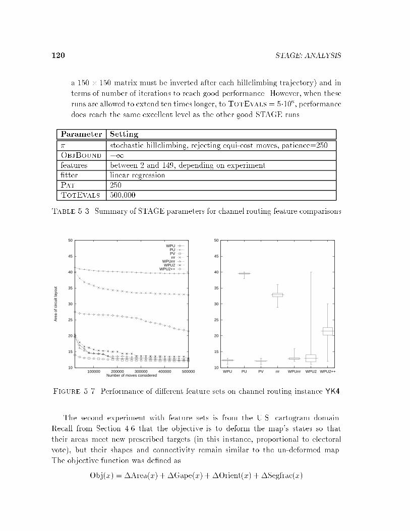
120 STAGE: ANALYSIS
a 150 � 150 matrix must be inverted after each hillclimbing trajectory) and in
terms of number of iterations to reach good performance. However, when these
runs are allowed to extend ten times longer, to TotEvals = 5�106, performance
does reach the same excellent level as the other good STAGE runs.
Parameter Setting
� stochastic hillclimbing, rejecting equi-cost moves, patience=250ObjBound �1features between 2 and 149, depending on experiment�tter linear regressionPat 250TotEvals 500,000
Table 5.3. Summary of STAGE parameters for channel routing feature comparisons
10
15
20
25
30
35
40
45
50
100000 200000 300000 400000 500000
Are
a of
circ
uit l
ayou
t
Number of moves considered
WPUPUPVrrr
WPUrrrWPU2
WPU2++
10
15
20
25
30
35
40
45
50
WPU PU PV rrr WPUrrr WPU2 WPU2++
Figure 5.7. Performance of di�erent feature sets on channel routing instance YK4
The second experiment with feature sets is from the U.S. cartogram domain.
Recall from Section 4.6 that the objective is to deform the map's states so that
their areas meet new prescribed targets (in this instance, proportional to electoral
vote), but their shapes and connectivity remain similar to the un-deformed map.
The objective function was de�ned as
Obj(x) = �Area(x) + �Gape(x) + �Orient(x) + �Segfrac(x)

x5.2 EMPIRICAL STUDIES OF PARAMETER CHOICES 121
Instance Algorithm Performance (50 runs each) RMSmean best worst of �t
YK4 WPU 12.34�0.15 11 13 2.7PU 39.54�0.16 38 40 2.8PV 12.08�0.10 11 13 2.8rrr 32.86�0.56 29 36 3.7WPUrrr 12.80�0.22 12 16 2.7WPU2 12.92�1.11 11 40 2.7WPU2++ 21.44�1.20 12 30 1.7
Table 5.4. Results with di�erent feature sets on channel routing instance YK4
and STAGE used those four subcomponents of the objective function as its features for
learning. Many other features can be imagined for this domain; I examine STAGE's
performance with several of them here. These experiments used linear regression to
�t ~V �. Other STAGE parameters are detailed in Table 5.5, and the results are shown
in Figure 5.8 and Table 5.6. The feature sets compared are as follows:
Asp.1: hAsp(x)i, a single feature describing the aspect ratio of the current map's
bounding rectangle. Note that most moves leave this feature unchanged. STAGE
learns a coe�cient near zero for this feature, and its performance of Obj � 0:16
is about the same as that of multi-restart hillclimbing.
Peri.1: hPeri(x)i, a single feature which sums the perimeter over all the states.
STAGE works surprisingly well with this feature. It learns a positive coe�-
cient on Peri(x); that is, it learns that hillclimbing performs better when it
begins from a map which is \scrunched."
Cop.2: the horizontal and vertical coordinates of map x's center of population. I
thought these would be a good pair of features for the US49 domain, since a
good cartogram should have its population center near the geometric center of
the map. However, these features were ine�ective, under both linear regression
(shown in graphs) and quadratic regression (not shown).
Obj.4: hArea(x);Gape(x);Orient(x);SegFrac(x)i, the four subcomponents of the ob-
jective function. These features worked quite well, though not as well as Peri.1
on average. Note that the better STAGE results of Section 4.6 used quadratic
regression over these four features.
ObjPeri.5: Given the good performance of Peri.1 and Obj.4, it is natural to combine
122 STAGE: ANALYSIS
them into a 5-feature representation for STAGE. This feature set performed
comparably to experiment Obj.4.
St.15: This larger feature set concentrates on �ve \important" states of the map:
New York, Texas, Florida, California, and Illinois. For each of these it provides
three features: the horizontal and vertical coordinates of the state's current
centroid (expressed relative to the map's current bounding rectangle) and the
state's area. Note that this is the �rst feature set I have tailored speci�cally
to this instance. However, STAGE's performance with these features, while
better than multi-restart hillclimbing, is worse than with most of the simple
instance-independent feature sets discussed above.
St.147: This experiment includes the three centroid and area features for all 49 of
the map's states. With this many features, STAGE is signi�cantly slowed down.
For a �xed number of moves, however, solution quality is signi�cantly better
than multi-restart hillclimbing.
This series of experiments shows that for almost any natural choice of domain features,
STAGE is able to discover a structure over those features which can be exploited to
improve performance signi�cantly over multi-restart hillclimbing.
Parameter Setting
� stochastic hillclimbing, rejecting equi-cost moves, patience=200ObjBound 0features between 1 and 147, depending on experiment�tter linear regressionPat 200TotEvals 1,000,000
Table 5.5. Summary of STAGE parameters for cartogram feature comparisons.
From the experiments reported here on the channel routing and cartogram do-
mains, and from other informal experiments not shown, I conclude that STAGE works
best with small, simple sets of features. Small feature sets not only are speediest for
STAGE to work with, but can also, in cases such as cartogram Experiment Peri.1,
provide a bias toward good extrapolation by ~V �, enabling successful exploration. Fea-
tures associated with subcomponents of the objective function, or the variance of such
subcomponents, were often helpful. With the function approximators tested here,
STAGE is not overly sensitive to the inclusion of extra random features; however, it

x5.2 EMPIRICAL STUDIES OF PARAMETER CHOICES 123
0
0.1
0.2
0.3
0.4
0.5
200000 400000 600000 800000 1e+06
Map
err
or fu
nctio
n
Number of moves considered
(HC)Asp.1Peri.1Cop.2Obj.4
ObjPeri.5St.15
St.147
0
0.1
0.2
0.3
0.4
0.5
(HC) Asp.1 Peri.1 Cop.2 Obj.4 ObjPeri.5 St.15 St.147
Figure 5.8. Cartogram performance with di�erent feature sets
Instance Algorithm Performance (50 runs each)mean best worst
US49 Asp.1 0.158�0.004 0.120 0.185Peri.1 0.067�0.004 0.052 0.144Cop.2 0.187�0.008 0.096 0.246Obj.4 0.092�0.011 0.039 0.170ObjPeri.5 0.085�0.008 0.045 0.210St.15 0.132�0.007 0.091 0.206St.147 0.109�0.009 0.064 0.205
Table 5.6. Cartogram results with di�erent feature sets

124 STAGE: ANALYSIS
can sometimes be drawn into abysmal performance even worse than multi-restart hill-
climbing by a particularly bad set of features, as in channel routing Experiment PU.
5.2.2 Fitters
Another key parameter to STAGE is the function approximator or \�tter" used to
model V �(x). In Section 3.4.3, I argued that �tters having a linear architecture,
such as polynomial regression (of any degree), are best suited to STAGE. Here, I
empirically investigate the performance of STAGE with a range of polynomial �t-
ters, ranging from degree 1 to degree 5, on both the channel routing and cartogram
domains.
The table below lists the eight �tters I tested. Let hf1; f2; : : : ; fDi denote the
features of each domain given to STAGE; note that D = 3 in the channel routing
domain and D = 4 in the cartogram domain. For each �tter, the table also gives the
total number of coe�cients being �t, both as a function of arbitrary D and in the
case where D = 4.
Key Description # params
F1: linear regression D + 1 = 5
F2: quadratic regression�D+22
�= 15
F3: cubic regression�D+33
�= 35
F4: quartic regression�D+44
�= 70
E2: quadratic regression without cross-terms.For each domain feature fi, this model in-cludes the terms fi and f2i but no cross-terms involving the product of more thanone feature.
2D + 1 = 9
E3: cubic regression without cross-terms 3D + 1 = 13E4: quartic regression without cross-terms 4D + 1 = 17E5: quintic regression without cross-terms 5D + 1 = 21
Results are given in the usual form in Tables 5.7 and 5.8 and Figures 5.9 and 5.9.
On both domains, the results indicate that the choice of �tter has a relatively minor
impact on performance. On the channel routing domain, slightly better results and
fewer poor outlier runs were obtained from the most highly biased models, linear
regression and crossterm-less quadratic regression. This is consistent with our earlier
observation that the linear approximation V �(x) � 10w(x) + 0:5p(x) � 10U(x) � 80
su�ces for excellent performance here. On the cartogram domain, however, somewhat
more complex models performed slightly better.
In these experiments, STAGE's computational overhead for function approxima-
tion was not a signi�cant component of running time, even for the most complex
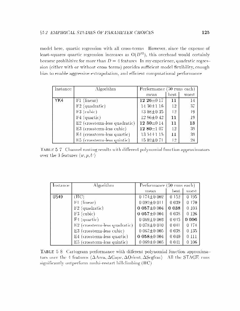
x5.2 EMPIRICAL STUDIES OF PARAMETER CHOICES 125
model here, quartic regression with all cross-terms. However, since the expense of
least-squares quartic regression increases as O(D12), this overhead would certainly
become prohibitive for more than D = 4 features. In my experience, quadratic regres-
sion (either with or without cross terms) provides su�cient model exibility, enough
bias to enable aggressive extrapolation, and e�cient computational performance.
Instance Algorithm Performance (50 runs each)mean best worst
YK4 F1 (linear) 12.26�0.17 11 14F2 (quadratic) 14.30�1.16 12 37F3 (cubic) 13.08�0.35 12 19F4 (quartic) 12.86�0.42 11 19E2 (crossterm-less quadratic) 12.30�0.14 11 13E3 (crossterm-less cubic) 12.80�1.07 12 39E4 (crossterm-less quartic) 13.54�1.15 11 39E5 (crossterm-less quintic) 15.02�0.71 12 24
Table 5.7. Channel routing results with di�erent polynomial function approximatorsover the 3 features hw; p; Ui
Instance Algorithm Performance (50 runs each)mean best worst
US49 (HC) 0.174�0.002 0.152 0.195F1 (linear) 0.092�0.011 0.039 0.170F2 (quadratic) 0.057�0.004 0.038 0.103F3 (cubic) 0.057�0.004 0.038 0.126F4 (quartic) 0.069�0.003 0.045 0.096E2 (crossterm-less quadratic) 0.078�0.010 0.041 0.174E3 (crossterm-less cubic) 0.067�0.005 0.038 0.135E4 (crossterm-less quartic) 0.058�0.004 0.040 0.111E5 (crossterm-less quintic) 0.069�0.005 0.041 0.106
Table 5.8. Cartogram performance with di�erent polynomial function approxima-tors over the 4 features h�Area;�Gape;�Orient;�Segfraci. All the STAGE runssigni�cantly outperform multi-restart hillclimbing (HC).

126 STAGE: ANALYSIS
10
15
20
25
30
35
40
45
50
0 50000100000150000200000250000300000350000400000450000500000
Are
a of
circ
uit l
ayou
t
Number of moves considered
F1F2F3F4E2E3E4E5
10
15
20
25
30
35
40
45
50
F1 F2 F3 F4 E2 E3 E4 E5
Figure 5.9. Performance of di�erent function approximators on channel routinginstance YK4
0
0.1
0.2
0.3
0.4
0.5
0 1000002000003000004000005000006000007000008000009000001e+06
Map
err
or fu
nctio
n
Number of moves considered
(HC)F1F2F3F4E2E3E4E5
0
0.1
0.2
0.3
0.4
0.5
(HC) F1 F2 F3 F4 E2 E3 E4 E5
Figure 5.10. Cartogram performance with di�erent polynomial function approxi-mators

x5.2 EMPIRICAL STUDIES OF PARAMETER CHOICES 127
5.2.3 Policy �
Thus far, I have discussed how the user's choice of features and �tters a�ects STAGE's
ability to learn and exploit ~V �(F (x)). But what about the choice of � itself? In
every domain of Chapter 4 besides Boolean satis�ability, � was chosen to be a very
simple search procedure: stochastic �rst-improvement hillclimbing, rejecting equi-
cost moves. But clearly, stronger local search procedures are available. For example,
stochastic hillclimbing accepting equi-cost moves often performs better, and simulated
annealing performs better still. Can STAGE learn to improve upon these, and achieve
yet better performance?
Theoretically, even if a procedure �1 is signi�cantly better than another procedure
�2, it is by no means guaranteed that STAGE on �1 will outperform STAGE on
�2. For example, �2 may produce more diverse outcomes as a function of starting
state, enabling useful extrapolation in ~V �2; whereas if �1 is expected to reach the
same solution quality no matter what state it starts from|as was the case with the
Boggle example of Section 5.1.4|then ~V �1 will be at, and STAGE will not produce
improvement.
In this section, I consider the following three policies on the cartogram domain:
� �1: regular �rst-improvement hillclimbing, rejecting equi-cost moves, patience=200.
� �2: hillclimbing as above, but modi�ed so that equi-cost and some slightly
harmful moves are accepted. Speci�cally, a move is rejected if and only if it
worsens Obj by more than �=0.0001. (This value of � was the most e�ective
of a wide range tried on this domain.) On average, �2 performs signi�cantly
better than �1.
� �3: simulated annealing with a shortened schedule length of 20,000 moves. The
short schedule allows it to be used in the context of a multi-restart procedure.
For each of these three policies, I sought to compare the default restarting method to
a \smart" restarting method learned by STAGE. In the cases of �1 and �2, the default
restarting method is to reset to the domain's initial state (the original undeformed
U.S. map). In the case of �3, I found that a better default restarting method is to
start each new annealing schedule in the same state where the previous trajectory
�nished. These procedures are labelled PI1, PI2 and PI3 in the results presented
below.
In applying STAGE to �2 and �3, a complication arises: neither of these proce-
dures is Markovian. Methods for coping with this theoretical di�culty were discussed

128 STAGE: ANALYSIS
in detail at the end of Section 3.4.1 (p. 61), and in the context of WALKSAT in Sec-
tion 4.7.2. In the case of �2, a simple �x is to train V �2(x) on only those states which
are the best-so-far on their trajectory. (Note that on the pure hillclimbing trajecto-
ries generated by �1, every state is the best-so-far.) These procedures are labelled
STAGE(PI1) and STAGE(PI2) in the results. In the case of �3, even training only
on best-so-far states does not make V �3(x) theoretically well-de�ned (though results
for STAGE(PI3) are given below nonetheless). Instead, giving up on the Markov
property, I resort to training V �3 on just the single starting state of each simulated
annealing trajectory. This variant of STAGE is well-de�ned for any proper policy �;
its results for all three of our policies are shown as STAGE0(PI1), STAGE0(PI2), and
STAGE0(PI3).
The results, displayed in Table 5.9 and Figures 5.11{5.13, point to several conclu-
sions. First, as demonstrated by Experiment STAGE(PI2), STAGE can successfully
learn from a non-Markovian policy by training only on best-so-far states. Second,
from Experiment STAGE(PI3) we can conclude that STAGE may not be e�ective
at learning evaluation functions from simulated annealing; this is unsurprising, since
SA's initial period of random search makes the outcome quite unpredictable from
the starting state. Third, from the set of STAGE0 experiments, it is apparent that
STAGE learns muchmore quickly when it is able to train on entire trajectories, rather
than just starting states. Thus, STAGE is able to exploit the Markov property of V �
for e�cient performance.
Instance Algorithm Performance (50 runs each)mean best worst
US49 PI1 = hillclimbing 0.174�0.002 0.152 0.192STAGE(PI1) 0.057�0.004 0.038 0.103STAGE0(PI1) 0.099�0.013 0.042 0.174PI2 = hillclimbing/�=0.0001 0.140�0.003 0.115 0.167STAGE(PI2) 0.052�0.003 0.040 0.083STAGE0(PI2) 0.077�0.009 0.045 0.136PI3 = simulated annealing 0.049�0.001 0.044 0.070STAGE(PI3) 0.050�0.002 0.042 0.091STAGE0(PI3) 0.060�0.005 0.043 0.142
Table 5.9. Cartogram performance with STAGE learning ~V � from a variety ofdi�erent choices of policy �. All algorithms were limited to considering TotEvals =106 moves.

x5.2 EMPIRICAL STUDIES OF PARAMETER CHOICES 129
0
0.1
0.2
0.3
0.4
0.5
200000 400000 600000 800000 1e+06
Map
err
or fu
nctio
n
Number of moves considered
PI1STAGE(PI1)
STAGE0(PI1)
0
0.1
0.2
0.3
0.4
0.5
PI1 STAGE(PI1) STAGE0(PI1)
Figure 5.11. Cartogram performance of STAGE using �1 = hillclimbing
0
0.1
0.2
0.3
0.4
0.5
200000 400000 600000 800000 1e+06
Map
err
or fu
nctio
n
Number of moves considered
PI2STAGE(PI2)
STAGE0(PI2)
0
0.1
0.2
0.3
0.4
0.5
PI2 STAGE(PI2) STAGE0(PI2)
Figure 5.12. Cartogram performance of STAGE using �2 = hillclimbing acceptingequi-cost and slightly harmful moves
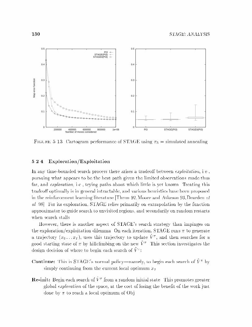
130 STAGE: ANALYSIS
0
0.1
0.2
0.3
0.4
0.5
200000 400000 600000 800000 1e+06
Map
err
or fu
nctio
n
Number of moves considered
PI3STAGE(PI3)
STAGE0(PI3)
0
0.1
0.2
0.3
0.4
0.5
PI3 STAGE(PI3) STAGE0(PI3)
Figure 5.13. Cartogram performance of STAGE using �3 = simulated annealing
5.2.4 Exploration/Exploitation
In any time-bounded search process there arises a tradeo� between exploitation, i.e.,
pursuing what appears to be the best path given the limited observations made thus
far, and exploration, i.e., trying paths about which little is yet known. Treating this
tradeo� optimally is in general intractable, and various heuristics have been proposed
in the reinforcement learning literature [Thrun 92,Moore and Atkeson 93,Dearden et
al. 98]. For its exploration, STAGE relies primarily on extrapolation by the function
approximator to guide search to unvisited regions, and secondarily on random restarts
when search stalls.
However, there is another aspect of STAGE's search strategy than impinges on
the exploration/exploitation dilemma. On each iteration, STAGE runs � to generate
a trajectory (x0 : : : xT ), uses this trajectory to update ~V �, and then searches for a
good starting state of � by hillclimbing on the new ~V �. This section investigates the
design decision of where to begin each search of ~V �:
Continue: This is STAGE's normal policy|namely, to begin each search of ~V � by
simply continuing from the current local optimum xT .
Re-init: Begin each search of ~V � from a random initial state. This promotes greater
global exploration of the space, at the cost of losing the bene�t of the work just
done by � to reach a local optimum of Obj.
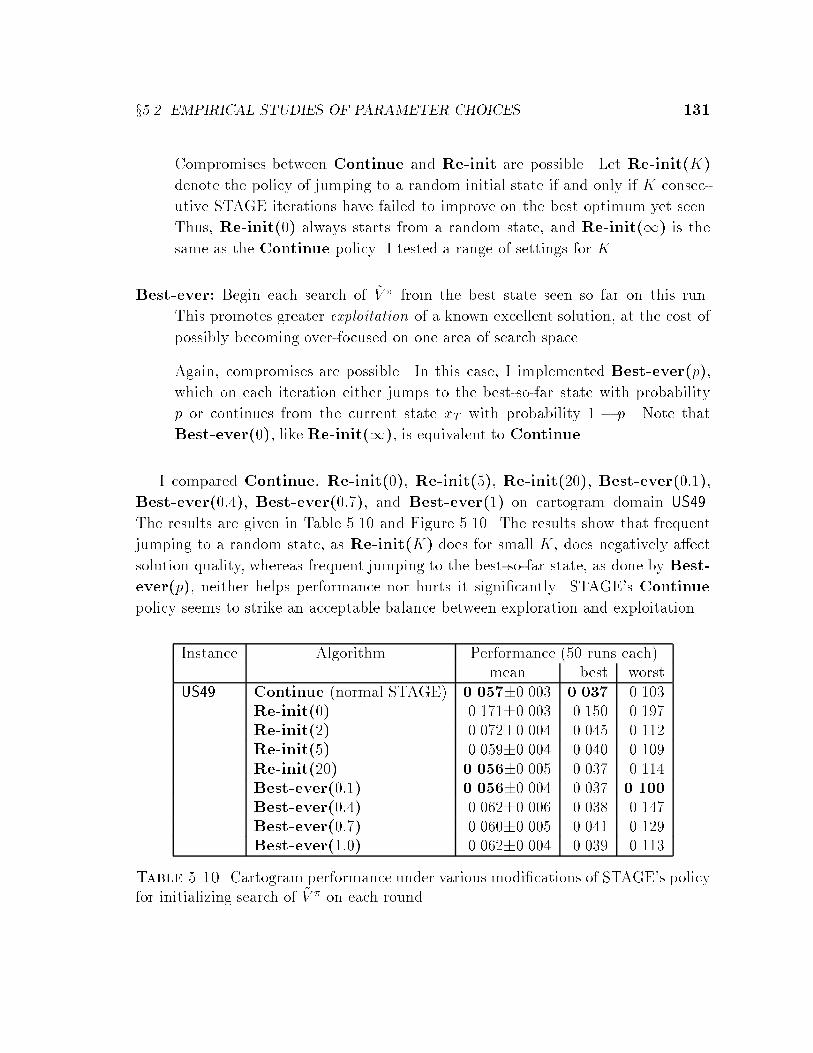
x5.2 EMPIRICAL STUDIES OF PARAMETER CHOICES 131
Compromises between Continue and Re-init are possible. Let Re-init(K)
denote the policy of jumping to a random initial state if and only if K consec-
utive STAGE iterations have failed to improve on the best optimum yet seen.
Thus, Re-init(0) always starts from a random state, and Re-init(1) is the
same as the Continue policy. I tested a range of settings for K.
Best-ever: Begin each search of ~V � from the best state seen so far on this run.
This promotes greater exploitation of a known excellent solution, at the cost of
possibly becoming over-focused on one area of search space.
Again, compromises are possible. In this case, I implemented Best-ever(p),
which on each iteration either jumps to the best-so-far state with probability
p or continues from the current state xT with probability 1 � p. Note that
Best-ever(0), like Re-init(1), is equivalent to Continue.
I compared Continue, Re-init(0), Re-init(5), Re-init(20), Best-ever(0:1),
Best-ever(0:4), Best-ever(0:7), and Best-ever(1) on cartogram domain US49.
The results are given in Table 5.10 and Figure 5.10. The results show that frequent
jumping to a random state, as Re-init(K) does for small K, does negatively a�ect
solution quality, whereas frequent jumping to the best-so-far state, as done by Best-
ever(p), neither helps performance nor hurts it signi�cantly. STAGE's Continue
policy seems to strike an acceptable balance between exploration and exploitation.
Instance Algorithm Performance (50 runs each)mean best worst
US49 Continue (normal STAGE) 0.057�0.003 0.037 0.103Re-init(0) 0.171�0.003 0.150 0.197Re-init(2) 0.072�0.004 0.045 0.112Re-init(5) 0.059�0.004 0.040 0.109Re-init(20) 0.056�0.005 0.037 0.114Best-ever(0:1) 0.056�0.004 0.037 0.100Best-ever(0:4) 0.062�0.006 0.038 0.147Best-ever(0:7) 0.060�0.005 0.041 0.129Best-ever(1:0) 0.062�0.004 0.039 0.113
Table 5.10. Cartogram performance under various modi�cations of STAGE's policyfor initializing search of ~V � on each round

132 STAGE: ANALYSIS
0
0.1
0.2
0.3
0.4
0.5
200000 400000 600000 800000 1e+06
Map
err
or fu
nctio
n
Number of moves considered
ContRe(0)Re(2)Re(5)
Re(20)Be(0.1)Be(0.4)Be(0.7)
Be(1)
0
0.1
0.2
0.3
0.4
0.5
Cont Re(0) Re(2) Re(5) Re(20) Be(0.1)Be(0.4)Be(0.7) Be(1)
Figure 5.14. Cartogram performance under various modi�cations of STAGE's pol-icy for initializing search of ~V � on each round
5.2.5 Patience and ObjBound
Finally, I investigated the e�ect of the two remaining STAGE parameters: Pat and
ObjBound. Recall from the STAGE algorithm (p. 52) that these parameters jointly
determine when STAGE's second phase of search, stochastic hillclimbing on ~V �,
should terminate. ObjBound corresponds to a known lower bound on the objec-
tive function; it cuts the search o� when ~V �(F (x)) predicts that x is an impossibly
good starting state, i.e., ~V �(F (x)) < ObjBound. This cuto� may be disabled by
setting ObjBound = �1. The other parameter, Pat, cuts the search o� when too
many consecutive moves have failed to improve ~V �. If either of these parameters is
set too aggressively (too tight a bound, too-low patience), then STAGE will fail to
reach the best starting points predicted by its function approximator. If, on the other
hand, these are set too loosely, then STAGE may waste valuable time that could in-
stead have been spent on the �rst phase of search, namely, running � and gathering
new training data. How sensitive is STAGE to the precise settings used?
Experimental results of varying these parameters on the cartogram domain are
presented in Table 5.11 and Figures 5.15 and 5.16. STAGE's other parameters were
set as in the cartogram experiments of Section 4.6 (p. 95). The results show that
STAGE's performance su�ered when Pat was very low or very high, but worked well
for a wide range of settings between 64 and 1024. As for the ObjBound parameter,

x5.3 DISCUSSION 133
STAGE performed best when it was set to its true bound of 0, but degraded gracefully
when it was set to �1 (too loose a bound) or +0:1 (too tight). Performance was,
however, signi�cantly worse for ObjBound=1, demonstrating that the ObjBound
parameter is useful. By cutting o� search on ~V � when the function approximator is
provably inaccurate, ObjBound saves computation time and prevents search from
wandering too far astray.
Instance Algorithm Performance (50 runs each)mean best worst
US49 Pat=16 0.161�0.015 0.079 0.285Pat=32 0.095�0.008 0.040 0.147Pat=64 0.065�0.006 0.040 0.151Pat=128 0.057�0.004 0.039 0.114Pat=256 0.059�0.007 0.038 0.190Pat=512 0.062�0.006 0.041 0.134Pat=1024 0.070�0.005 0.044 0.126Pat=2048 0.100�0.006 0.046 0.159Pat=4096 0.126�0.008 0.074 0.187Pat=8192 0.122�0.007 0.057 0.172Pat=16384 0.132�0.006 0.068 0.178Pat=32768 0.129�0.007 0.079 0.189Pat=65536 0.135�0.007 0.081 0.184ObjBound=�1 0.083�0.011 0.036 0.189ObjBound=�1 0.060�0.006 0.037 0.143ObjBound=0 0.057�0.004 0.038 0.103ObjBound=0:1 0.061�0.006 0.040 0.171
Table 5.11. Cartogram performance with varying settings of Pat and ObjBound
5.3 Discussion
This chapter gives depth to the results of the previous chapter, demonstrating that
STAGE does indeed obtain its success by exploiting the power of reinforcement learn-
ing, and that it works reliably over a wide range of parameter settings. The chapter's
empirical conclusions may be summarized as follows:
� Evaluation functions other than STAGE's learned ~V �, built at random or by
simply smoothing the objective function, perform much worse than ~V � in the
context of multi-start optimization. STAGE successfully learns and ex-
ploits the predictive power of value functions.
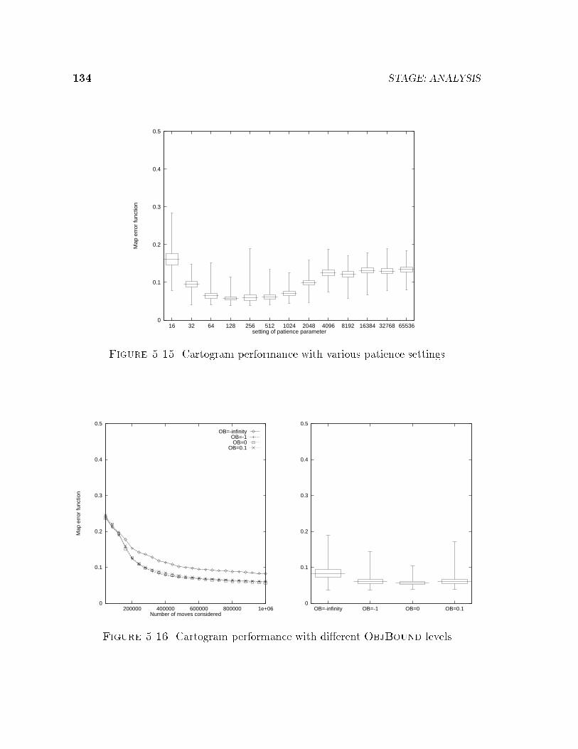
134 STAGE: ANALYSIS
0
0.1
0.2
0.3
0.4
0.5
16 32 64 128 256 512 1024 2048 4096 8192 16384 32768 65536
Map
err
or fu
nctio
n
setting of patience parameter
Figure 5.15. Cartogram performance with various patience settings
0
0.1
0.2
0.3
0.4
0.5
200000 400000 600000 800000 1e+06
Map
err
or fu
nctio
n
Number of moves considered
OB=-infinityOB=-1OB=0
OB=0.1
0
0.1
0.2
0.3
0.4
0.5
OB=-infinity OB=-1 OB=0 OB=0.1
Figure 5.16. Cartogram performance with di�erent ObjBound levels
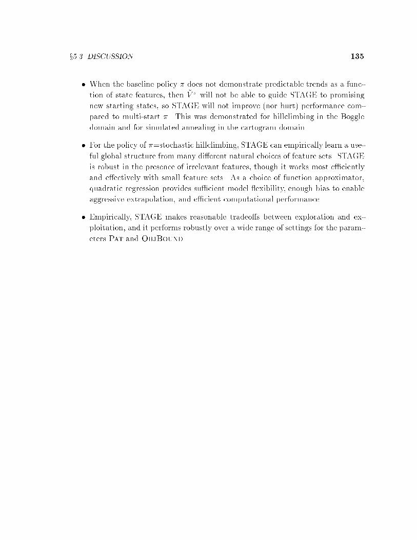
x5.3 DISCUSSION 135
� When the baseline policy � does not demonstrate predictable trends as a func-
tion of state features, then ~V � will not be able to guide STAGE to promising
new starting states, so STAGE will not improve (nor hurt) performance com-
pared to multi-start �. This was demonstrated for hillclimbing in the Boggle
domain and for simulated annealing in the cartogram domain.
� For the policy of �=stochastic hillclimbing, STAGE can empirically learn a use-
ful global structure from many di�erent natural choices of feature sets. STAGE
is robust in the presence of irrelevant features, though it works most e�ciently
and e�ectively with small feature sets. As a choice of function approximator,
quadratic regression provides su�cient model exibility, enough bias to enable
aggressive extrapolation, and e�cient computational performance.
� Empirically, STAGE makes reasonable tradeo�s between exploration and ex-
ploitation, and it performs robustly over a wide range of settings for the param-
eters Pat and ObjBound.

136

137
Chapter 6
STAGE: Extensions
The preceding chapters have demonstrated the e�ectiveness of a simple idea:
learned predictions of search outcomes can be used to improve future search out-
comes. In this chapter, I consider two independent extensions to the basic STAGE
algorithm:
� Section 6.1 investigates the use of the TD(�) family of algorithms, including
a new least-squares formulation, for making more e�cient use of memory and
data while learning V �.
� Section 6.2 illustrates how STAGE's training time on a problem instance may
be reduced by transferring learned ~V � functions from previously solved, similar
problem instances.
6.1 Using TD(�) to learn V�
In almost all of the experimental results of Chapters 4 and 5, STAGE learned to
approximate V � for a particularly simple choice of �: stochastic hillclimbing with
equi-cost moves rejected. This procedure is proper, Markovian, and monotonic, and
therefore|as shown earlier in Section 3.4.1|induces a Markov chain over the con�g-
uration space X. V �(x) is precisely the value function of the chain.
To approximate V �, STAGE uses simple Monte-Carlo simulation and linear least-
squares function approximation, as described in [Bertsekas and Tsitsiklis 96, x6.2.1].
However, a reinforcement learning technique, TD(�) or temporal di�erence learning,
also applies. TD(�) is a family of incremental gradient-descent algorithms for approx-
imating V �, parametrized by � 2 [0; 1] [Sutton 88]. For the case of � = 0, Bradtke
and Barto [96] demonstrated improved data e�ciency with a least-squares formula-
tion of the algorithm, which he called LSTD(0). LSTD(0) also eliminates all stepsize
parameters from the TD procedure.
In this section, I generalize Bradtke and Barto's results to arbitrary values of
� 2 [0; 1], drawing on the analyses of TD(�) in [Tsitsiklis and Roy 96,Bertsekas and
Tsitsiklis 96]. I show that LSTD(1) produces the same coe�cients as Monte-Carlo
138 STAGE: EXTENSIONS
simulation with linear regression, but requires less memory (and no extra computa-
tion). I also explain how LSTD(�) bridges the gap between model-free and model-
based RL algorithms. Finally, I demonstrate empirical results with STAGE in the
Bayes net structure-�nding domain, showing that LSTD(�) with � set to values less
than 1 can sometimes learn an e�ective approximation of V � from less simulation
data than supervised linear regression.
6.1.1 TD(�): Background
TD(�) addresses the problem of computing the value function V � of a Markov chain,
or equivalently, of a �xed policy � in a Markov Decision Problem. This is an important
subproblem of several algorithms for sequential decision making, including policy
iteration [Bertsekas and Tsitsiklis 96] and STAGE. V �(x) simply predicts the expected
long-term sum of future rewards obtained when starting from state x and following
policy � until termination. This function is well-de�ned as long as � is proper, i.e.,
guaranteed to terminate.1
For small Markov chains whose transition probabilities are all explicitly known,
computing V � is a trivial matter of solving a system of linear equations; TD(�) is not
needed. However, in many practical applications, the transition probabilities of the
chain are available only implicitly: either in the form of a simulation model or in the
form of an agent's actual experience executing � in its environment. In either case, we
must compute V � or an approximation to V � solely from a collection of trajectories
sampled from the chain. This is where the TD(�) family of algorithms applies.
TD(�) was introduced in [Sutton 88]; excellent summaries may now be found in
several books [Bertsekas and Tsitsiklis 96,Sutton and Barto 98]. For each state on an
observed trajectory (x0; x1; : : : ; xL;end), TD(�) incrementally adjusts the coe�cients
of ~V � to more closely satisfy
~V �(xt):= (1� �)
L�1Xk=t
�k�t�~V �(xk+1) +
Pkj=tRj
�+
�L�t�PL
j=tRj
� (6.1)
where Rj is a shorthand for the one-step reward R(xj; xj+1). The right hand side of
Equation 6.1 can be interpreted as computing the weighted average of L� t di�erent
lookahead-based estimates for ~V �(xt). The di�erent estimates are the 1-step trun-
cated return (Rt + ~V �(xt+1)), 2-step truncated return Rt + Rt+1 + ~V �(xt+2), and so
1For improper policies, V � may be made well-de�ned by the use of a discount factor that expo-nentially reduces future rewards; the TD(�) and LSTD(�) algorithms both extend straightforwardlyto that case. However, for simplicity I will assume here that V � is undiscounted and that � is proper.

x6.1 USING TD(�) TO LEARN V � 139
forth up to the total Monte-Carlo return (Rt+Rt+1+ � � �+RL). The relative weights
of these estimates are determined by the terms involving �, which sum to unity. The
� parameter smoothly interpolates between two extremes:
� TD(1): adjust ~V � based only on the Monte-Carlo return. This gives rise to an
incremental form of supervised learning.
� TD(0): adjust ~V � based only on the 1-step lookahead Rt + ~V �(xt+1). This
gives rise to an incremental, sampled form of Value Iteration.
The target values assigned by TD(1) are unbiased samples of ~V �, but may have
signi�cant variance since each depends on a long sequence of rewards from stochastic
transitions. By contrast, TD(0)'s target values have low variance|the only random
component is the reward of a single state transition|but are biased by the potential
inaccuracy of the current estimate of ~V �. The parameter � trades o� between bias
and variance. Empirically, intermediate values of � seem to perform best [Sutton
88,Singh and Sutton 96,Sutton 96].
A convenient form of the TD(�) algorithm is given in Table 6.1.1. This version
of the algorithm assumes that the policy � is proper, that the approximation archi-
tecture is linear (as described in Section 3.4.3), and that updates are o�ine (i.e., the
coe�cients of ~V � are modi�ed only at the end of each trajectory). On each transition,
the algorithm computes the scalar one-step TD error Rt + (�(xt+1)��(xt))T�, and
apportions that error among all state features according to their respective eligibilities
zt. The eligibility vector may be seen as an algebraic trick by which TD(�) propa-
gates rewards backward over the current trajectory without having to remember the
trajectory explicitly. Each feature's eligibility at time t depends on the trajectory's
history and on �:
zt =
tXk=t0
�t�k�(xk)
where t0 is the time when the current trajectory started. In the case of TD(0), only
the current state's features are eligible to be updated, so zt = �(xt); whereas in
TD(1), the features of all states seen so far on the current trajectory are eligible, so
zt =Pt
k=t0�(xk).
The reason for the restriction to linear approximation architectures is that TD(�)
provably converges when such architectures are used, under a few mild additional as-
sumptions detailed below [Tsitsiklis and Roy 96]. The currently available convergence
results may be summarized as follows [Bertsekas and Tsitsiklis 96]:
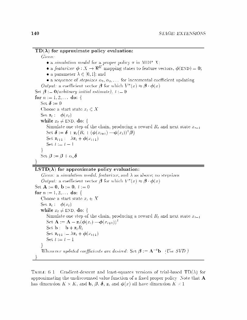
140 STAGE: EXTENSIONS
TD(�) for approximate policy evaluation:Given:� a simulation model for a proper policy � in MDP X;� a featurizer � : X ! <K mapping states to feature vectors, �(end) = 0;� a parameter � 2 [0; 1]; and� a sequence of stepsizes �1; �2; : : : for incremental coe�cient updating.
Output: a coe�cient vector � for which V �(x) � � � �(x).Set � := 0(arbitrary initial estimate); t := 0.for n := 1; 2; : : : do: f
Set � := 0.Choose a start state xt 2 X.Set zt := �(xt).while xt 6= end, do: f
Simulate one step of the chain, producing a reward Rt and next state xt+1.Set � := � + zt
�Rt + (�(xt+1)� �(xt))
T��.
Set zt+1 := �zt + �(xt+1).Set t := t+ 1.
gSet � := � + �n�.
g
LSTD(�) for approximate policy evaluation:Given: a simulation model, featurizer, and � as above; no stepsizes.Output: a coe�cient vector � for which V �(x) � � � �(x).
Set A := 0; b := 0; t := 0.for n := 1; 2; : : : do: f
Choose a start state xt 2 X.Set zt := �(xt).while xt 6= end, do: f
Simulate one step of the chain, producing a reward Rt and next state xt+1.Set A := A + zt(�(xt)� �(xt+1))
T.Set b := b+ ztRt.Set zt+1 := �zt + �(xt+1).Set t := t+ 1.
gWhenever updated coe�cients are desired: Set � := A�1b. (Use SVD.)
g
Table 6.1. Gradient-descent and least-squares versions of trial-based TD(�) forapproximating the undiscounted value function of a �xed proper policy. Note that Ahas dimension K �K, and b, �, �, z, and �(x) all have dimension K � 1.

x6.1 USING TD(�) TO LEARN V � 141
� If the approximator is nonlinear, TD(�) may diverge [Bertsekas and Tsitsiklis
96], though it has been successful with nonlinear neural networks in practice.
� If the function approximator is linear and can represent the optimal V � exactly,
then TD(�) will converge to V �. This result applies primarily to representations
with one independent feature per state, i.e., lookup tables.
� If the approximator is linear but cannot represent V � exactly, then TD(1) will
converge to the best least-squares �t of V �. For values of � < 1, TD(�) will
also converge, but possibly to a suboptimal �t of V �; the error bound worsens
as � decreases toward zero [Bertsekas and Tsitsiklis 96]. In practice, though,
smaller values of � introduce less variance and may enable TD(�) to converge
to an acceptable approximation of V � using less data.
Su�cient conditions for the convergence, with probability 1, of TD(�) are as follows:
1. The stepsizes �n are nonnegative, satisfyP1
n=1 �n =1, and satisfyP1
n=1 �2n <
1. (The stepsizes �n = c=n satisfy this condition, though in practice a small
constant stepsize is often used.)
2. All states x 2 X have positive probability of being visited given the start state
distribution chosen. (This is a technicality: unvisited states may simply be
deleted from the chain.)
3. The features �(x) are linearly independent of one another over X. That is, the
feature set is not redundant.
What does TD(�) converge to? Examining the update rule for � in Table 6.1.1,
it is not di�cult to see that the coe�cient changes made by TD(�) after an observed
trajectory (x0; x1; : : : ; xL;end) have the form
� := � + �n(d+C� + !)
where
d = E� LXi=0
ziR(xi; xi+1)
C = E� LXi=0
zi��(xi+1)��(xi)
�T! = zero-mean noise.
142 STAGE: EXTENSIONS
The expectations are taken with respect to the distribution of trajectories through
the Markov chain. It is shown in [Bertsekas and Tsitsiklis 96] that C is negative
de�nite and that the noise ! has su�ciently small variance, which together with the
stepsize conditions given above, imply that � converges to a �xed point �� satisfying
d+C�� = 0:
In e�ect, TD(�) solves this system of equations by performing stochastic gradient
descent on the potential function k� � ��k2. It never explicitly represents d or C.
The changes to � depend only on the most recent trajectory, and after those changes
are made, the trajectory and its rewards are simply forgotten. This approach, while
requiring little computation time per iteration, is wasteful with data and may require
sampling many trajectories to reach convergence.
One technique for using data more e�ciently is \experience replay" [Lin 93]: ex-
plicitly remember all trajectories ever seen, and whenever asked to produce an up-
dated set of coe�cients, perform repeated passes of TD(�) over all the saved tra-
jectories until convergence. This technique is similar to the batch training methods
commonly used to train neural networks. However, in the case of linear function
approximators, there is another way.
6.1.2 The Least-Squares TD(�) Algorithm
The Least-Squares TD(�) algorithm, or LSTD(�), converges to the same coe�cients
�� that TD(�) does. However, instead of performing gradient descent, LSTD(�)
builds explicit estimates of the C matrix and d vector (actually, estimates of a con-
stant multiple of C and d), and then e�ectively solves d +C�� = 0 directly. The
actual data structures that LSTD(�) builds from experience are the matrix A (of
dimensionK�K, where K is the number of features) and the vector b (of dimension
K):
b =tX
i=0
ziR(xi; xi+1)
A =tX
i=0
zi��(xi)� �(xi+1)
�TAfter n independent trajectories have been observed, b is an unbiased estimate of
nd, and A is an unbiased estimate of �nC. Thus, �� can be estimated as A�1b.
As in the least-squares linear regression technique of Section 3.4.3, I use Singular
Value Decomposition to invert A robustly [Press et al. 92]. The complete LSTD(�)
algorithm is speci�ed in the bottom half of Table 6.1.1.

x6.1 USING TD(�) TO LEARN V � 143
LSTD(�) is a generalization of the LSTD(0) algorithm [Bradtke and Barto 96] to
the case of arbitrary �. When � = 0, the equations reduce to
b =tX
i=0
�(xi)R(xi; xi+1)
A =tX
i=0
�(xi)��(xi)� �(xi+1)
�T;
(6.2)
the same as those derived by Bradtke and Barto using a di�erent approach based on
regression with instrumental variables [Bradtke and Barto 96].
At the other extreme, when � = 1, LSTD(1) produces precisely the same A
and b as would be produced by supervised linear regression on training pairs of
(state features 7! observed eventual outcomes), as described for STAGE in Chapter 3
(Equation 3.8, page 67). The proof of this equivalence is given in Appendix A.2.
Thanks to the algebraic trick of the eligibility vectors, LSTD(1) builds the regression
matrices fully incrementally|without having to store the trajectory while waiting to
observe the eventual outcome. When trajectories through the chain are long, this
provides signi�cant memory savings over linear regression.
The computation per timestep required to update A and b is the same as least-
squares linear regression: O(K2), where K is the number of features. LSTD(�) must
also perform a matrix inversion at a cost of O(K3) whenever �'s coe�cients are
needed|in the case of STAGE, once per complete trajectory. (If updated coe�-
cients are required more frequently, then the O(K3) cost can be avoided by recursive
least-squares [Bradtke and Barto 96] or Kalman-�ltering techniques [Bertsekas and
Tsitsiklis 96, x3.2.2], which update � on each timestep at a cost of only O(K2).)
LSTD(�) is more computationally expensive than incremental TD(�), which updates
the coe�cients using only O(K) computation per timestep. However, LSTD(�) o�ers
several signi�cant advantages, as pointed out by Bradtke and Barto in their discussion
of LSTD(0) [96]:
� Least-squares algorithms are \more e�cient estimators in the statistical sense"
because \they extract more information from each additional observation."
� TD(�)'s convergence can be slowed dramatically by a poor choice of the stepsize
parameters �n. LSTD(�) eliminates these parameters.
� TD(�)'s performance is sensitive to k�� � �initk, the distance between �� and
the initial estimate for ��. LSTD(�) requires no arbitrary initial estimate.
� TD(�) is also sensitive to the ranges of the individual features. LSTD(�) is not.
144 STAGE: EXTENSIONS
Section 6.1.4 below presents experimental results comparing TD(�) with LSTD(�) in
terms of data e�ciency and time e�ciency.
6.1.3 LSTD(�) as Model-Based TD(�)
Before giving experimental results with LSTD(�), I would like to point out an in-
teresting connection between LSTD(�) and model-based reinforcement learning. To
begin, let us restrict our attention to the case of a small discrete state space X,
over which V � can be represented and learned exactly by a lookup table. A classical
model-based algorithm for learning V � from simulated trajectory data would proceed
as follows:
1. From the state transitions and rewards observed so far, build in memory an
empirical model of the Markov chain. The su�cient statistics of this model
consist of, for each state x 2 X:
� n(x), the number of times state x was visited;
� c(x0jx), the count of how many times x0 followed x for each state x0 2 X.
We do not need to track the absorption frequency c(endjx) separately,
since c(endjx) = n(x)�P
x02X c(x0jx).
� s(x), the sum of all observed one-step rewards from state x. (The expected
reward at x is then given simply by s(x)=n(x).)
2. Whenever a new estimate of the value function V � is desired, solve the current
empirical model. Solving the model means solving the linear system of Bellman
equations (Eq. 2.3), which can be written in the above notation as, 8x 2 X:
V �(x) =s(x)
n(x)+Xx02X
c(x0jx)
n(x)V �(x0) (6.3)
In matrix notation, if we let N be the diagonal matrix of visitation frequencies
n(x), let C be the matrix of counts where Cij = c(xjjxi), let s be the vector
of summed-rewards s(x), and let v be the vector of V � values, then the above
equations become simply
Nv = s+Cv;
whose solution is given by
v = (N�C)�1s: (6.4)

x6.1 USING TD(�) TO LEARN V � 145
This model-based technique contrasts with TD(�), a model-free approach to the same
problem. TD(�) does not maintain any statistics on observed transitions and rewards;
it simply updates the components of v incrementally after each observed trajectory.
In the limit, assuming a lookup-table representation, both converge to the optimal
V �. The advantage of TD(�) is its low computational burden per step; the advantage
of the classical model-based method is that it makes the most of the available training
data. The empirical advantages of model-based and model-free reinforcement learning
methods have been investigated in, e.g., [Sutton 90,Moore and Atkeson 93,Atkeson
and Santamaria 97,Kuvayev and Sutton 97].
Where does LSTD(�) �t in? The answer is that, when � = 0, it precisely du-
plicates the classical model-based method sketched above. When � > 0, it does
something else sensible, which I describe below; but let us �rst consider LSTD(0).
The assumed lookup-table representation for ~V � means that we have one indepen-
dent feature per state: the feature vector � corresponding to state 1 is (1; 0; 0; : : : ; 0);
corresponding to state 2 is (0; 1; 0; : : : ; 0); etc. LSTD(0) performs the following op-
erations upon each observed transition (cf. Equation 6.2):
b := b+ �(xt)Rt
A := A+ �(xt)(�(xt)� �(xt+1))T
Clearly, the role of b is to sum all the rewards observed at each state, exactly as the
vector s does in the classical technique. A, meanwhile, accumulates the statistics
(N�C). To see this, note that the outer product given above is a matrix consisting
of an entry of +1 on the single diagonal element corresponding to state xt; an entry
of �1 on the element in row xt, column xt+1; and all the rest zeroes. Summing one
such sparse matrix for each observed transition gives A � N�C. Finally, LSTD(0)
performs the inversion � := A�1b = (N � C)�1s, giving the same solution as in
Equation 6.4.
Thus, when � = 0, the A and b matrices built by LSTD(�) e�ectively record a
model of all the observed transitions. What about when � > 0? Again, A and b
record the su�cient statistics of an empirical Markov model|but in this case, the
model being captured is one whose single-step transition probabilities directly encode
the multi-step TD(�) backup operations, as de�ned by Eq. 6.1. That is, the model
links each state x to all the downstream states that follow x on any trajectory, and
records how much in uence each has on estimating ~V �(x) according to TD(�). In the
case of � = 0, the TD(�) backups correspond to the one-step transitions, resulting
in the equivalence described above. The opposite extreme, the case of � = 1, is
also interesting: the empirical Markov model corresponding to TD(1)'s backups is

146 STAGE: EXTENSIONS
the chain where each state x leads directly to absorption (i.e., all counts are zero:
C1 = 0). The values s1(x) equal the sum, over all visits to x on all trajectories, of
all the observed rewards between x and termination. LSTD(1) then solves for ~V � as
follows:
� := A�1b = (N�C1)�1s1 = N�1s1;
which simply computes the average of the Monte-Carlo returns at each state x. In
short, if we assume a lookup-table representation for the function ~V �, we can view
the LSTD(�) algorithm as doing these two steps:
1. It implicitly uses the observed simulation data to build a Markov chain. This
chain compactly models all the backups that TD(�) would perform on the data.
2. It solves the chain by performing a matrix inversion.
The lookup-table representation for ~V � is intractable in practical problems; in
practice, LSTD(�) operates on states only via their (linearly dependent) feature rep-
resentations �(x). In this case, we can view LSTD(�) as implicitly building a com-
pressed version of the empirical model's transition matrixN�C and summed-reward
vector s:
A = �T(N�C)�
b = �Ts;
where � is the jXj�K matrix representation of the function � : X ! <K. From the
compressed empirical model, LSTD(�) computes the following coe�cients for ~V �:
�� = A�1b
= (�T(N�C)�)�1(�Ts):(6.5)
Ideally, these coe�cients �� would be equivalent to the empirical optimal coe�cients
���. The empirical optimal coe�cients are those that would be found by building the
full uncompressed empirical model (represented by N � C and s), using a lookup
table to solve for that model's value function (v = (N�C)�1s), and then performing
a least-squares linear �t from the state features � to the lookup-table value function:
��� = (�T�)�1(�Tv)
= (�T�)�1�T(N�C)�1s:(6.6)
It can be seen that Equations 6.5 and 6.6 are indeed equivalent for the case of � = 1,
because that setting of � implies that C = 0 so (N�C) is diagonal. However, for the
case of � < 1, solving the compressed empirical model does not in general produce
the optimal least-squares �t to the solution of the uncompressed model.
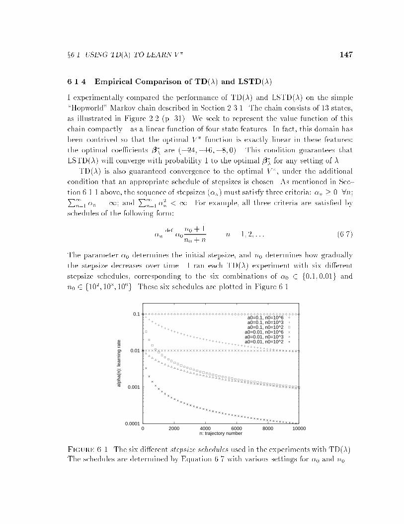
x6.1 USING TD(�) TO LEARN V � 147
6.1.4 Empirical Comparison of TD(�) and LSTD(�)
I experimentally compared the performance of TD(�) and LSTD(�) on the simple
\Hopworld" Markov chain described in Section 2.3.1. The chain consists of 13 states,
as illustrated in Figure 2.2 (p. 31). We seek to represent the value function of this
chain compactly|as a linear function of four state features. In fact, this domain has
been contrived so that the optimal V � function is exactly linear in these features:
the optimal coe�cients ��� are (�24;�16;�8; 0). This condition guarantees that
LSTD(�) will converge with probability 1 to the optimal ��� for any setting of �.
TD(�) is also guaranteed convergence to the optimal V �, under the additional
condition that an appropriate schedule of stepsizes is chosen. As mentioned in Sec-
tion 6.1.1 above, the sequence of stepsizes (�n) must satisfy three criteria: �n � 0 8n;P1n=1 �n = 1; and
P1n=1 �
2n < 1. For example, all three criteria are satis�ed by
schedules of the following form:
�ndef= �0
n0 + 1
n0 + nn = 1; 2; : : : (6.7)
The parameter �0 determines the initial stepsize, and n0 determines how gradually
the stepsize decreases over time. I ran each TD(�) experiment with six di�erent
stepsize schedules, corresponding to the six combinations of �0 2 f0:1; 0:01g and
n0 2 f102; 103; 106g. These six schedules are plotted in Figure 6.1.
0.0001
0.001
0.01
0.1
0 2000 4000 6000 8000 10000
alph
a(n)
: lea
rnin
g ra
te
n: trajectory number
a0=0.1, n0=10^6a0=0.1, n0=10^3a0=0.1, n0=10^2
a0=0.01, n0=10^6a0=0.01, n0=10^3a0=0.01, n0=10^2
Figure 6.1. The six di�erent stepsize schedules used in the experiments with TD(�).The schedules are determined by Equation 6.7 with various settings for �0 and n0.

148 STAGE: EXTENSIONS
On the Hopworld domain, I ran both TD(�) and LSTD(�) for a variety of settings
of �. Figure 6.2 plots the results for the case of � = 0:4. The plot compares the
performance of six variants of TD(0:4)|corresponding to the six di�erent stepsize
schedules|and LSTD(0:4). The x-axis counts the number of trajectories sampled,
up to a limit of 10,000; and the y-axis measures the RMS error of the approximated
value function ~V �, de�ned by
k~V � � V �k =
1
jXj
Xx2X
�~V �(x)� V �(x)
�2! 12
: (6.8)
Each point on the plot represents the average of 10 trials.
0
0.2
0.4
0.6
0.8
1
100 1000 10000
RM
S e
rror
of V
pi o
ver
all s
tate
s
trajectory number
lambda = 0.4
TD: a0=0.1, n0=10^6TD: a0=0.1, n0=10^3TD: a0=0.1, n0=10^2
TD: a0=0.01, n0=10^6TD: a0=0.01, n0=10^3TD: a0=0.01, n0=10^2
Least-Squares TD
Figure 6.2. Performance of TD(0:4) and LSTD(0:4) on the Hopworld domain. Notethe logarithmic scale of the x-axis.
The plot shows clearly that for � = 0:4, LSTD(�) learns a good approximation to
V � in fewer trials than any of the TD(�) experiments, and performs better asymp-
totically as well. These results held uniformly across all values of �. Table 6.2 gives
the results for � = 0, � = 0:4, and � = 1. The results may be summarized as follows:
� For all values of �, the convergence rate of LSTD(�) exceeded that of TD(�).

x6.1 USING TD(�) TO LEARN V � 149
AlgorithmFit errorafter 100trajectories
Fit errorafter 10,000trajectories
TD(0), �0 = 0:1; n0 = 106 0.49� 0.15 0.37� 0.05TD(0), �0 = 0:1; n0 = 103 0.38� 0.10 0.09� 0.02TD(0), �0 = 0:1; n0 = 102 0.32� 0.07 0.04� 0.02TD(0), �0 = 0:01; n0 = 106 9.08� 0.04 0.10� 0.02TD(0), �0 = 0:01; n0 = 103 9.29� 0.04 0.04� 0.02TD(0), �0 = 0:01; n0 = 102 10.66� 0.02 0.70� 0.01LSTD(0) 0.19� 0.09 0.01� 0.01TD(0:4), �0 = 0:1; n0 = 106 0.42� 0.15 0.40� 0.09TD(0:4), �0 = 0:1; n0 = 103 0.39� 0.16 0.12� 0.04TD(0:4), �0 = 0:1; n0 = 102 0.25� 0.08 0.03� 0.01TD(0:4), �0 = 0:01; n0 = 106 6.73� 0.07 0.14� 0.04TD(0:4), �0 = 0:01; n0 = 103 6.97� 0.06 0.04� 0.01TD(0:4), �0 = 0:01; n0 = 102 8.73� 0.04 0.17� 0.01LSTD(0:4) 0.15� 0.04 0.01� 0.00TD(1), �0 = 0:1; n0 = 106 0.73� 0.27 0.54� 0.15TD(1), �0 = 0:1; n0 = 103 0.48� 0.20 0.17� 0.06TD(1), �0 = 0:1; n0 = 102 0.30� 0.10 0.06� 0.02TD(1), �0 = 0:01; n0 = 106 1.86� 0.14 0.13� 0.03TD(1), �0 = 0:01; n0 = 103 2.05� 0.14 0.05� 0.02TD(1), �0 = 0:01; n0 = 102 3.31� 0.12 0.03� 0.01LSTD(1) 0.14� 0.04 0.01� 0.00
Table 6.2. Summary of results with TD(�) and LSTD(�) on the Hopworld domainfor � = 0, 0.4, and 1.0. Fit errors are measured according to Equation 6.8; the meanover 10 trials and 95% con�dence interval of the mean are displayed. Results for othervalues of � were similar.
150 STAGE: EXTENSIONS
� The performance of TD(�) depends critically on the stepsize schedule chosen.
LSTD(�) has no tunable parameters other than � itself.
� Varying � had no discernible e�ect on LSTD(�)'s performance.
Because the Hopworld domain is so small and the optimal value function is exactly
linear over the available features, these results are not necessarily representative of
how TD(�) and LSTD(�) will perform on practical problems. For example, if a
domain has many features and simulation data is available cheaply, then incremental
methods will have better real-time performance than least-squares methods [Sutton
92]. On the other hand, some reinforcement-learning applications have been successful
with very small numbers of features (e.g., [Singh and Bertsekas 97]). STAGE's results
certainly meet this description. I investigate the performance of LSTD(�) in the
context of STAGE in the following section.
One exciting possibility for future work is to apply LSTD(�) in the context of
Markov decision problems|that is, for the purpose of approximating not V � but
V �. LSTD(�) could provide an e�cient alternative to TD(�) in the inner loop of
optimistic policy iteration [Bertsekas and Tsitsiklis 96].
6.1.5 Applying LSTD(�) in STAGE
The application of LSTD(�) within STAGE is straightforward. We are given a local
search procedure � that is assumed to be proper, Markovian and monotonic, which
implies that � induces a Markov chain over the con�guration space X. (To use
LSTD(�) with a nonmonotonic local search procedure such as WALKSAT, the best-
so-far abstraction must be applied; see Appendix A.1.) Note that the one-step rewards
in the induced Markov chain are all zero except at termination (see Eq. 3.4, p. 59).
This means that the update step b := b+ ztRt may be moved outside the inner loop
of LSTD(�).
The interesting empirical question concerns the best value of �. The STAGE
experiments of Chapters 4 and 5 all used supervised least-squares regression, which
is equivalent to � = 1. Is that value of � best, since the predictions it generates
are unbiased estimates of the true V � function? Or will a lower setting of � enable
learning in fewer trials, since LSTD(�)'s implicit transition model enables it to treat
noisy training data more informedly?
I performed experiments with LSTD(�) on three optimization problem instances:
cartogram design instance US49 and Bayes net structure-�nding instances SYNTH125K
and ADULT2. Other than �, all STAGE parameters were �xed at the same settings

x6.1 USING TD(�) TO LEARN V � 151
speci�ed earlier in Sections 4.4 and 4.6. The � parameter was varied over six evenly-
spaced settings between 0 and 1.
The experimental results, shown in Table 6.3 and the accompanying three �gures,
were inconclusive. On the cartogram design problem, LSTD(1) decisively outper-
formed all the smaller values of �. By contrast, on SYNTH125K, all values of � � 0:8
produced signi�cantly faster learning than LSTD(1), although Figure 6.4 shows that
LSTD(1) nearly catches up by the time 100,000 moves have been considered. Fi-
nally, on instance ADULT2, there were no signi�cant di�erences between any of the
di�erent settings for �. From this set of results, the most that can be said is that
values of � < 1 sometimes help, sometimes hurt, and sometimes have no e�ect on the
performance of STAGE in practice.
Instance Algorithm Performance (N runs each)mean best worst
Cartogram LSTD(0:0) 0.083�0.008 0.040 0.178(US49) LSTD(0:2) 0.078�0.009 0.040 0.183N = 50;M = 106 LSTD(0:4) 0.074�0.007 0.041 0.170
LSTD(0:6) 0.079�0.010 0.038 0.204LSTD(0:8) 0.076�0.007 0.042 0.175LSTD(1:0) 0.057�0.004 0.037 0.105
Bayes net LSTD(0:0) 736241� 1721 720244 784874(SYNTH125K) LSTD(0:2) 734806� 1722 719431 777711N = 200;M = 4 � 104 LSTD(0:4) 734548� 1674 719187 779267
LSTD(0:6) 736164� 1938 719261 796555LSTD(0:8) 736094� 1796 719068 776308LSTD(1:0) 741111� 1871 719748 790014
Bayes net LSTD(0:0) 440511� 59 439372 441052(ADULT2) LSTD(0:2) 440531� 62 439460 441247N = 100;M = 105 LSTD(0:4) 440540� 60 439761 441168
LSTD(0:6) 440490� 52 439767 441208LSTD(0:8) 440484� 67 439267 441152LSTD(1:0) 440461� 61 439715 441005
Table 6.3. STAGE performance with LSTD(�) on three optimization instances.Each line summarizes the performance of N trials, each limited to considering Mtotal search moves.

152 STAGE: EXTENSIONS
0
0.1
0.2
0.3
0.4
0.5
200000 400000 600000 800000 1e+06
Map
err
or fu
nctio
n
Number of moves considered
TD(0.0)TD(0.2)TD(0.4)TD(0.6)TD(0.8)TD(1.0)
0
0.1
0.2
0.3
0.4
0.5
TD(0.0) TD(0.2) TD(0.4) TD(0.6) TD(0.8) TD(1.0)
Figure 6.3. Cartogram performance with LSTD(�)
720000
740000
760000
780000
800000
20000 40000 60000 80000 100000
Bay
es n
et s
core
Number of moves considered
TD(0.0)TD(0.2)TD(0.4)TD(0.6)TD(0.8)TD(1.0)
720000
740000
760000
780000
800000
0.0 0.2 0.4 0.6 0.8 1.0
lambda
Performance after 40,000 moves considered
Figure 6.4. Performance of STAGE with LSTD(�) on Bayes net structure-�ndinginstance SYNTH125K. After 40; 000 moves, LSTD(1:0) signi�cantly lagged all othervalues for �.

x6.2 TRANSFER 153
439000
440000
441000
442000
443000
444000
445000
20000 40000 60000 80000 100000
Bay
es n
et s
core
Number of moves considered
TD(0.0)TD(0.2)TD(0.4)TD(0.6)TD(0.8)TD(1.0)
439000
440000
441000
442000
443000
444000
445000
0.0 0.2 0.4 0.6 0.8 1.0
lambda
Figure 6.5. Performance of STAGE with LSTD(�) on Bayes net structure-�ndinginstance ADULT2
6.2 Transfer
This section concerns a second signi�cant extension to STAGE: enabling transfer
of learned knowledge between related problem instances. I motivate and describe
an algorithm for transfer, X-STAGE, and present empirical results on two problem
families.
6.2.1 Motivation
There is a computational cost to training a function approximator on V �. Learn-
ing from a �-trajectory of length L, with either linear regression or LSTD(�) over
D features, costs STAGE O(D2L + D3) per iteration; quadratic regression costs
O(D4L+D6). In the experiments of Chapter 4, these costs were minimal|typically,
0{10% of total execution time. However, STAGE's extra overhead would become
signi�cant if many more features or more sophisticated function approximators were
used. Furthermore, even if the function approximation is inexpensive, STAGE may
require many trajectories to be sampled in order to obtain su�cient data to �t V �
e�ectively.
For some problems such costs are worth it in comparison with a non-learning
method, because a better or equally good solution is obtained with overall less com-
putation. But in those cases where we use more computation, the STAGE method

154 STAGE: EXTENSIONS
may nevertheless be preferable if we are then asked to solve further similar problems
(e.g., a new channel routing problem with di�erent pin assignments). Then we can
hope that the computation we invested in solving the �rst problem will pay o� in the
second, and future, problems because we will already have a ~V � estimate. This e�ect
is called transfer ; the extent to which it occurs is largely an empirical question.
To investigate the potential for transfer, I re-ran STAGE on a suite of eight prob-
lems from the channel routing literature [Chao and Harper 96]. Table 6.4 summarizes
the results and gives the coe�cients of the linear evaluation function, learned inde-
pendently for each problem. To make the similarities easier to see in the table, I have
normalized the coe�cients so that their squares sum to one; note that the search
behavior of an evaluation function is invariant under positive linear transformations.
Problem lower best-of-3 best-of-3 learned coe�cientsinstance bound hillclimbing STAGE < �w; �p; �U >YK4 10 22 12 < 0:71; 0:05; �0:70 >HYC1 8 8 8 < 0:52; 0:83; �0:19 >HYC2 9 9 9 < 0:71; 0:21; �0:67 >HYC3 11 12 12 < 0:72; 0:30; �0:62 >HYC4 20 27 23 < 0:71; 0:03; �0:71 >HYC5 35 39 38 < 0:69; 0:14; �0:71 >HYC6 50 56 51 < 0:70; 0:05; �0:71 >HYC7 39 54 42 < 0:71; 0:13; �0:69 >HYC8 21 29 25 < 0:71; 0:03; �0:70 >
Table 6.4. STAGE results on eight problems from [Chao and Harper 96]. Thecoe�cients have been normalized so that their squares sum to one.
The similarities among the learned evaluation functions are striking. Except on
the trivially small instance HYC1, all the STAGE-learned functions assign a relatively
large positive weight to feature w(x), a similarly large negative weight to feature U(x),
and a small positive weight to feature p(x). In Section 5.1.3 (see Eq. 5.1, page 116),
I explained the coe�cients found on instance YK4 as follows: STAGE has learned
that good hillclimbing performance is predicted by an uneven distribution of track
fullness levels (w(x) � U(x)) and by a low analytical bound on the e�ect of further
merging of tracks (p(x)). From Table 6.4, we can conclude that this explanation
holds generally for many channel routing instances. Thus, transfer between instances
should be fruitful.
x6.2 TRANSFER 155
6.2.2 X-STAGE: A Voting Algorithm for Transfer
Many sensible methods for transferring the knowledge learned by STAGE from \train-
ing" problem instances to new instances can be imagined. This section presents one
such method. STAGE's learned knowledge, of course, is represented by the approxi-
mated value function ~V �. We would like to take the ~V � information learned on a set of
training instances fI1; I2; : : : ; INg and use it to guide search on a given new instance
I 0. But how can we ensure that ~V � is meaningful across multiple problem instances
simultaneously, when the various instances may di�er markedly in size, shape, and
attainable objective-function value?
The �rst crucial step is to impose an instance-independent representation on the
features F (x), which comprise the input to ~V �(F (x)). In their algorithm for transfer
between job-shop scheduling instances (which I will discuss in detail in Section 7.2),
Zhang and Dietterich recognize this: they de�ne \a �xed set of summary statistics
describing each state, and use these statistics as inputs to the function approximator"
[Zhang and Dietterich 98]. As it so happens, almost all the feature sets used with
STAGE in this thesis are naturally instance-independent, or can easily be made so
by normalization. For example, in Bayes-net structure-�nding problems (x4.4), the
feature that counts the number of \orphan" nodes can be made instance-independent
simply by changing it to the percentage of total nodes that are orphans.
The second question concerns normalization of the outputs of ~V �(F (x)), which
are predictions of objective-function values. In Table 6.4 above, the nine channel
routing instances all have quite di�erent solution qualities, ranging from 8 tracks
in the case of instance HYC1 to more than 50 tracks in the case of instance HYC6.
If we wish to train a single function approximator to make meaningful predictions
about the expected solution quality on both instances HYC1 and HYC6, then we must
normalize the objective function itself. For example, ~V � could be trained to predict
not the expected reachable Obj value, but the expected reachable percentage above
a known lower bound for each instance. Zhang and Dietterich adopt this approach:
they heuristically normalize each instance's �nal job-shop schedule length by dividing
it by the di�culty level of the starting state [Zhang and Dietterich 98]. This enables
them to train a single neural network over all problem instances.
However, if tight lower bounds are not available, such normalization can be prob-
lematic. Consider the following concrete example:
� There are two similar instances, I1 and I2, which both have the same true
optimal solution, say, Obj(x�) = 130.
� A single set of features f is equally good in both instances, promising to lead
156 STAGE: EXTENSIONS
search to a solution of quality 132 on either.
� The only available lower bounds for the two instances are b1 = 110 and b2 = 120,
respectively.
In this example, normalizing the objective functions to report a percentage above the
available lower bound would result in a target value of 20% for ~V �(f) on I1 and a
target value of 10% for ~V �(f ) on I2. At best, these disparate training values add
noise to the training set for ~V �. At worst, they could interact with other inaccurate
training set values and make the non-instance-speci�c ~V � function useless for guiding
search on new instances.
I adopt here a di�erent approach, which eliminates the need to normalize the
objective function across instances. The essential idea is to recognize that each in-
dividually learned ~V �Ikfunction, unnormalized, is already suitable for guiding search
on the new problem I 0: the search behavior of an evaluation function is scale- and
translation-invariant. The X-STAGE algorithm, speci�ed in Table 6.5, combines the
knowledge of multiple ~V �Ikfunctions not by merging them into a single new evaluation
function, but by having them vote on move decisions for the new problem I 0. Note
that after the initial set of value functions has been trained, X-STAGE performs no
further learning when given a new optimization problem I 0 to solve.
Combining ~V �Ikdecisions by voting rather than, say, averaging, ensures that each
training instance carries equal weight in the decision-making process, regardless of
the range of that instance's objective function. Voting is also robust to \outlier"
functions, such as the one learned on instance HYC1 in Table 6.4 above. Such a
function's move recommendations will simply be outvoted. A drawback to the voting
scheme is that, in theory, loops are possible in which a majority prefers x over x0,
x0 over x00, and x00 over x. However, I have not seen such a loop in practice, and if one
did occur, the patience counter Pat would at least prevent X-STAGE from getting
permanently stuck.
6.2.3 Experiments
I applied the X-STAGE algorithm to the domains of bin-packing and channel rout-
ing. For the bin-packing experiment, I gathered a set of 20 instances from the OR-
Library|the same 20 instances studied in Section 4.2. Using the same STAGE
parameters given in that section (p. 75), I trained ~V � functions for all of the 20
except u250 13, and then applied X-STAGE to test performance on the held-out in-
stance. The performance curves of X-STAGE and, for comparison, ordinary STAGE
are shown in Figure 6.6. The semilog scale of the plot clearly shows that X-STAGE
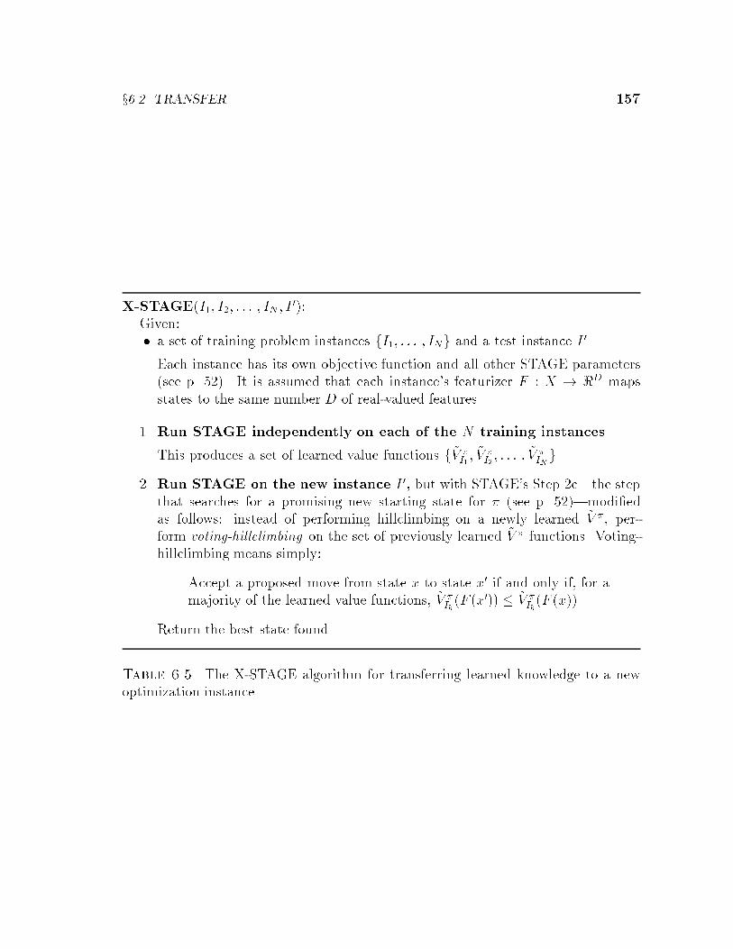
x6.2 TRANSFER 157
X-STAGE(I1; I2; : : : ; IN ; I 0):Given:� a set of training problem instances fI1; : : : ; INg and a test instance I 0.
Each instance has its own objective function and all other STAGE parameters(see p. 52). It is assumed that each instance's featurizer F : X ! <D mapsstates to the same number D of real-valued features.
1. Run STAGE independently on each of the N training instances.
This produces a set of learned value functions f~V �I1; ~V �
I2; : : : ; ~V �
INg.
2. Run STAGE on the new instance I 0, but with STAGE's Step 2c|the stepthat searches for a promising new starting state for � (see p. 52)|modi�edas follows: instead of performing hillclimbing on a newly learned ~V �, per-form voting-hillclimbing on the set of previously learned ~V � functions. Voting-hillclimbing means simply:
Accept a proposed move from state x to state x0 if and only if, for amajority of the learned value functions, ~V �
Ik(F (x0)) � ~V �
Ik(F (x)).
Return the best state found.
Table 6.5. The X-STAGE algorithm for transferring learned knowledge to a newoptimization instance

158 STAGE: EXTENSIONS
reaches good performance levelsmore quickly than STAGE. However, after only about
10 learning iterations and 10,000 evaluations, the average performance of STAGE
exceeds that of X-STAGE. STAGE's ~V � function, �nely tuned for the particular in-
stance under consideration, ultimately outperforms the voting-based restart policy
generated from 19 related instances.
105
110
115
120
125
1000 10000 100000
Num
ber
of b
ins
(103
is o
ptim
al)
Number of moves considered
STAGEX-STAGE
Figure 6.6. Bin-packing performance on instance u250 13 with transfer (X-STAGE)and without transfer (STAGE). Note the logarithmic scale of the x-axis.
The channel routing experiment was conducted with the set of 9 instances shown
in Table 6.4 above. Again, all STAGE parameters were set as in the experiments of
Chapter 4 (see p. 81). I trained ~V � functions for the instances HYC1 : : :HYC8, and
applied X-STAGE to test performance on instance YK4. The performance curves of
X-STAGE and ordinary STAGE are shown in Figure 6.7. Again, X-STAGE reaches
good performance levels more quickly than does STAGE. This time, the voting-based
restart policy maintains its superiority over the instance-speci�c learned policy for
the duration of the run.
These preliminary experiments indicate that the knowledge STAGE learns dur-
ing problem-solving can indeed be pro�tably transferred to novel problem instances.
Future work will consider ways of combining previously learned knowledge with new
knowledge learned during a run, so as to have the best of both worlds: exploiting

x6.3 DISCUSSION 159
10
15
20
25
30
35
40
45
50
5000 50000 500000
Are
a of
circ
uit l
ayou
t
Number of moves considered
STAGEX-STAGE
Figure 6.7. Channel routing performance on instance YK4 with transfer (X-STAGE)and without transfer (STAGE). Note the logarithmic scale of the x-axis.
general knowledge about a family of instances to reach good solutions quickly, and
exploiting instance-speci�c knowledge to reach the best possible solutions.
6.3 Discussion
This chapter has presented two signi�cant extensions to STAGE: the Least-Squares
TD(�) algorithm for e�cient reinforcement learning of ~V �; and the X-STAGE al-
gorithm for transferring ~V � functions learned on a set of problem instances to new,
similar instances. Many further interesting extensions to STAGE are possible. Af-
ter giving a survey of related work in Chapter 7, I will present a number of as-yet
unexplored ideas for STAGE in the concluding chapter.

160

161
Chapter 7
Related Work
Heuristic methods for global optimization have assuredly not been overlooked in
the literature. Their practical applications are important and numerous, and the
literature is correspondingly immense. There is also a signi�cant, if not quite as
overwhelming, literature on learning evaluation functions for heuristic search in game-
playing and problem-solving. In this chapter, I review the prior work most relevant
to STAGE from both these literatures. The reviewed topics are organized as follows:
� x7.1: adaptive multi-restart techniques for local search;
� x7.2: reinforcement learning for combinatorial optimization, especially the study
of Zhang and Dietterich [95];
� x7.3: simulation-based methods for improving AI search in game-playing and
problem-solving domains, including techniques based on \rollouts" and on learn-
ing evaluation functions; and
� x7.4: genetic algorithms.
I defer a high-level discussion of STAGE's novel contributions to the next, concluding
chapter.
7.1 Adaptive Multi-Restart Techniques
An iteration of hillclimbing typically reaches a local optimum very quickly. Thus, in
the time required to perform a single iteration of (say) simulated annealing, one can
run many hillclimbing iterations from di�erent random starting points (or even from
the same starting point, if move operators are sampled stochastically) and report
the best result. Empirically, random multi-start hillclimbing has produced excellent
solutions on practical computer vision tasks [Beveridge et al. 96], outperformed sim-
ulated annealing on the Traveling Salesman Problem (TSP) [Johnson and McGeoch
95], and outperformed genetic algorithms and genetic programming on several large-
scale testbeds [Juels and Wattenberg 96].

162 RELATED WORK
Nevertheless, the e�ectiveness of random multi-start local search is limited in
many cases by a \central limit catastrophe" [Boese et al. 94]: random local optima
in large problems tend to all have average quality, with little variance [Martin and
Otto 94]. This means the chance of �nding an improved solution diminishes quickly
from one iteration to the next. To improve on these chances, an adaptive multi-start
approach|designed to select restart states with better-than-average odds of �nding
an improved solution|seems appropriate. Indeed, in the theoretical model of local
search proposed by Aldous and Vazirani [94], a given performance level that takes
O(n) restarts to reach by a random starting policy can instead be reached with as
few as O(log n) restarts when an adaptive policy, which uses successful early runs to
seed later starting states, is used.
Many adaptive multi-start techniques have been proposed. One particularly rel-
evant study has recently been conducted by Boese [95, 96]. On a �xed, well-known
instance of the TSP, he ran local search 2500 times to produce 2500 locally optimal
solutions. Then, for each of those solutions, he computed the average distance to the
other 2499 solutions, measured by a natural distance metric on TSP tours. The results
showed a stunning correlation between solution quality and average distance: high-
quality local optima tended to have small average distance to the other optima|they
were \centrally" located|while worse local optima tended to have greater average
distance to the others; they were at the \outskirts" of the space. Similar correlations
were found in a variety of other optimization domains, including circuit/graph parti-
tioning, satis�ability, number partitioning, and job-shop scheduling. Boese concluded
that many practical optimization problems exhibit a \globally convex" or so-called
\big valley" structure, in which the set of local optima appears convex with one central
global optimum. Boese's intuitive diagram of the big valley structure is reproduced
in Figure 7.1.
The big valley structure is auspicious for a STAGE-like approach. Indeed, Boese's
intuitive diagram, motivated by his experiments on large-scale complex problems,
bears a striking resemblance to the 1-D wave function of Figure 3.4 (p. 48), which
I contrived as an example of the kind of problem at which STAGE would excel.
Working from the assumption of the big valley structure, Boese recommended the
following two-phase adaptive multi-start methodology for optimization:
Phase One: GenerateR random starting solutions and run Greedy Descent
from each to determine a set of corresponding random local minima.
Phase Two: Based on the local minima obtained so far, construct adap-
tive starting solutions and run Greedy DescentA times from each one
to yield corresponding adaptive local minima.

x7.1 ADAPTIVE MULTI-RESTART TECHNIQUES 163
Figure 7.1. Intuitive picture of the \big valley" solution space structure. (Adaptedfrom [Boese 95].)
Intuitively, the two phases respectively develop, then exploit, a structural
picture of the cost surface. [Boese et al. 94]
At this level of description, the two phases of Boese's recommended search regime
correspond almost exactly with the two alternating phases of STAGE. The main
di�erence is that Boese hand-builds a problem-speci�c routine for adaptively con-
structing new starting states, whereas STAGE uses machine learning to do the same
automatically. Another di�erence is that STAGE's learned heuristic for constructing
starting states is based on full hillclimbing trajectories, not just the local minima
obtained so far.
A similar methodology underlies the current best heuristic for solving large Travel-
ing Salesman problems, \Chained Local Optimization" (CLO) [Martin and Otto 94].
CLO performs ordinary hillclimbing to reach a local optimum z, and then applies
a special large-step stochastic operator designed to \kick" the search from z into a
nearby but di�erent attracting basin. Hillclimbing from this new starting point pro-
duces a new local optimum z0; if this turns out to be much poorer than z, then CLO
returns to z, undoing the kick. In e�ect, CLO constructs a new high-level search space:
the new operators consist of large-step kick moves, and the new objective function
is calculated by �rst applying hillclimbing in the low-level space, then evaluating the
resulting local optimum. (A similar trick is often applied with genetic algorithms, as
I discuss in Section 7.4 below.) In the TSP, the kick designed by Martin and Otto [94]
is a so-called \double-bridge" operation, chosen because such moves cannot be easily
found nor easily undone by Lin-Kernighan local search moves [Johnson and McGeoch
95]. Like Boese's adaptive multi-start, CLO relies on manually designed kick steps
for �nding a good new starting state, as opposed to STAGE's learned restart policy.

164 RELATED WORK
Furthermore, STAGE's \kicks" place search in not just a random nearby basin, but
one speci�cally predicted to produce an improved local optimum.
The big valley diagram, like my 1-D wave function, conveys the notion of a global
structure over the local optima. Unlike the wave function, it also conveys one poten-
tially misleading intuition: that starting from low-cost solutions is necessarily better
than starting from high-cost solutions. In his survey of local search techniques for the
TSP, Johnson [95] considered four di�erent randomized heuristics for constructing
starting tours from which to begin local search. He found signi�cant di�erences in
the quality of �nal solutions. Interestingly, the heuristic that constructed the best-
quality starting tours (namely, the \Clarke-Wright" heuristic) was also the one that
led search to the worst -quality �nal solutions|even worse than starting from a very
poor, completely random tour. Such \deceptiveness" can cause trouble for simulated
annealing and genetic algorithms. Large-step methods such as CLO may evade some
such deceits by \stepping over" high-cost regions. STAGE confronts the deceit head-
on: it explicitly detects when features other than the objective function are better
predictors of �nal solution quality, and can learn to ignore the objective function
altogether when searching for a good start state.
Many other sensible heuristics for adaptive restarting have been shown e�ective
in the literature. The widely applied methodology of \tabu search" [Glover and
Laguna 93] is fundamentally a set of adaptive heuristics for escaping local optima,
like CLO's kick steps. Hagen and Kahng's \Clustered Adaptive Multi-Start" achieves
excellent results on the VLSI netlist partitioning task [Hagen and Kahng 97]; like
CLO, it alternates between search with high-level operators (constructed adaptively
by clustering elements of previous good solutions) and ordinary local search. Jagota's
\Stochastic Steep Descent with Reinforcement Learning" heuristically rewards good
starting states and punishes poor starting states in a multi-start hillclimbing context
[Jagota et al. 96,Jagota 96]. The precise reward mechanism is heuristically determined
and appears to be quite problem-speci�c, as opposed to STAGE's uniform mechanism
of predicting search outcomes by value function approximation. As such, a direct
empirical comparison would be di�cult.
7.2 Reinforcement Learning for Optimization
Value function approximation has previously been applied to a large-scale combina-
torial optimization task: the Space Shuttle Payload Processing domain [Zhang and
Dietterich 95,Zhang 96]. I will discuss this application in some detail, because both
the similarities and di�erences to STAGE are instructive. Please refer back to Sec-
tion 2.1 for details on the algorithms and notation of value function approximation.

x7.2 REINFORCEMENT LEARNING FOR OPTIMIZATION 165
The Space Shuttle Payload Processing (SSPP) domain is a form of job-shop
scheduling: given a partially ordered set of jobs and the resources required by each,
assign them start times so as to respect the partial order, meet constraints on si-
multaneous resource usage, and minimize the total execution time. Following the
\repair-based scheduling" paradigm of Zweben [94], Zhang and Dietterich de�ned a
search over the space of fully speci�ed schedules that meet the ordering constraints
but not necessarily the resource constraints. Search begins at a �xed start state, the
\critical path schedule," and proceeds by the application of two types of determin-
istic operators: Reassign-Pool and Move. To keep the number of instantiated
operators small, they considered only operations which would repair the schedule's
earliest constraint violation. Search terminates as soon as a violation-free schedule is
reached.
Zhang and Dietterich applied reinforcement learning to this domain in order to
obtain transfer : their goal was to learn a value function which captured knowledge
about not a single instance of a scheduling problem, but rather a large family of
related scheduling instances. Thus, the input to their value function approximator
(a neural network) consisted of abstract instance-independent features, such as the
percentage of the schedule containing a violation and the mean and standard deviation
of certain slack times. Likewise, the ultimate measure of schedule quality which the
neural network was learning to predict had to be normalized so that it spanned the
same range regardless of problem di�culty. (The voting-based approach to transfer
introduced in Section 6.2.2 of this thesis allows such normalization to be avoided.)
Trained on many scheduling instances, the neural network could then be applied to
guide search on a novel scheduling instance, hopefully producing a good solution
quickly.
Unlike STAGE, which seeks to learn V �, the predicted outcome of a prespeci�ed
optimization policy �|the Zhang and Dietterich approach seeks to learn V �, the
predicted outcome of the best possible optimization policy. Before discussing how they
approached this ambitious goal, we must address how the \best possible optimization
policy" is even de�ned, since optimization policies face two con icting objectives:
\produce good solutions" and \�nish quickly." In the SSPP domain, Zhang and
Dietterich measured the total cost of a search trajectory (x0; x1; : : : ; xN ;end) by
Obj(xN) + 0:001N
E�ectively, since Obj(x) is near 1:0 in this problem, this cost function means that a
1% improvement in �nal solution quality is worth about 10 extra search steps [Zhang
and Dietterich 98]. The goal of learning, then, was to produce a policy �� to optimize
this balance between trajectory length and �nal solution quality.

166 RELATED WORK
Following Tesauro's methodology for learning V � on backgammon, Zhang and
Dietterich applied optimistic TD(�) to the SSPP domain. Rather than training only a
single neural network, they trained a pool of 8{12 networks, using di�erent parameter
settings for each. They trained the networks on a set of small problem instances.
Training continued until performance stopped improving on a validation set of other
problem instances. Then, the N best-performing networks were saved and used in a
round-robin fashion for comparisons against Zweben's iterative-repair system [Zweben
et al. 94], the previously best scheduler. The results showed that searches with the
learned evaluation functions produced schedules as good as Zweben's in less than half
the CPU time.
Getting these good results required substantial tuning. One complication involves
state-space cycles. Since the move operators are deterministic, a learned policy may
easily enter an in�nite loop, which makes its value function unde�ned. Loops are fairly
infrequent in the SSPP domain because most operators repair constraint violations,
lengthening the schedule; still, Zhang and Dietterich had to include a loop-detection
and escape mechanism, clouding the interpretation of V �. To attack other combina-
torial optimization domains with their method, they suggest that \it is important to
formulate problem spaces so that they are acyclic" [Zhang and Dietterich 98]|but
such formulations are unnatural for most local search applications, in which the op-
erators typically allow any solution to be reached from any other solution. STAGE
�nesses this issue by �xing � to be a proper policy such as hillclimbing.
STAGE also manages to �nesse three other algorithmic complications which Zhang
and Dietterich found it necessary to introduce: experience replay [Lin 93], random
exploration (slowly decreasing over time), and random-sample greedy search. Expe-
rience replay, i.e., saving the best trajectories in memory and occasionally retraining
on them, is unnecessary in STAGE because the regression matrices always maintain
the su�cient statistics of all historical training data. Adding random exploration
is unnecessary because empirically, STAGE's baseline policy � (e.g., stochastic hill-
climbing or WALKSAT) provides enough exploration inherently. This is in contrast
to the SSPP formulation, where actions are deterministic. Finally, STAGE does
not face the branching factor problem which led Zhang and Dietterich to introduce
random-sample greedy search (RSGS). Brie y, the problem is that when hundreds or
thousands of legal operators are available, selecting the greedy action, as optimistic
TD(�) requires, is too costly. RSGS uses a heuristic to select an approximately greedy
move from a subset of the available moves. Again, this clouds the interpretation of
V �. In STAGE, each decision is simply whether to accept or reject a single available
move, and the interpretation of V � is clear.

x7.3 ROLLOUTS AND LEARNING FOR AI SEARCH 167
To summarize, STAGE avoids most of the algorithmic complexities of Zhang and
Dietterich's method because it is solving a fundamentally simpler problem: estimat-
ing V � from a �xed stochastic �, rather than discovering an optimal deterministic
policy �� and value function V �. It also avoids many issues of normalizing problem
instances and designing training architectures by virtue of the fact that it applies in
the context of a single problem instance. However, an advantage of the Zhang and
Dietterich approach is that it holds out the potential of identifying a truly optimal
or near-optimal policy ��. STAGE can only claim to learn an improvement over the
prespeci�ed policy �.
Another published work, the \Ant-Q" system [Dorigo and Gambardella 95], is also
billed as a reinforcement learning approach to combinatorial optimization. Based on
an extensive metaphor with the behavior of ant colonies, it has been applied only to
the TSP; it is unclear how it would be applied to other optimization domains.
7.3 Rollouts and Learning for AI Search
Ordinary hillclimbing, simulated annealing and genetic algorithms evaluate the qual-
ity of each neighboring state x0 by its objective function value Obj(x0). STAGE
evaluates x0 by how promising its features make it appear, ~V �(F (x0)). A third possi-
bility is to evaluate x0 by performing one or more actual sample runs of hillclimbing
starting from x0. This is the principle of so-called \rollout algorithms" [Bertsekas et
al. 97, Tesauro and Galperin 97], a term borrowed from the backgammon-strategy
literature [Woolsey 91]. Like STAGE, rollout methods evaluate each neighbor based
upon its long-term promise as a starting state for a �xed policy �. Selecting ac-
tions in this way is tantamount to performing a single round of the policy iteration
algorithm [Howard 60] and can be guaranteed to improve upon � [Bertsekas et al. 97].
Unlike STAGE, rollout methods do not cache the results of their lookahead searches
in a function approximator ~V �. In this way they avoid the biases that feature represen-
tations and function approximation introduce, perhaps allowing more accurate moves.
However, the computational cost of replacing function approximator evaluations by
full sample runs is extremely high. This cost may be tolerable in a game-playing sce-
nario where several seconds are available for each move selection; but would probably
be deadly for practical optimization algorithms, where (in the words of Buntine [97])
a general maxim applies: \speed over smarts."
In fact, an earlier study of Abramson [90] demonstrated the power of rollout
methods for game-playing, although he was apparently unaware of the connection to
Markov decision processes and policy iteration. In his \expected-outcome" model,
moves in the game of Othello were made by computing, via multiple rollouts for each
168 RELATED WORK
legal move, the expected probability of winning assuming both sides play randomly
from that point on. Though this assumption is clearly inaccurate, Abramson reported
empirical good play at Othello:
Given no expert information, the ability to evaluate only leaves, and a
good deal of computation time, [expected-outcome functions] were able
to play better than a competent (albeit non-masterful) function that had
been handcrafted by an expert. [Abramson 90]
This improvement is consistent with the experience of Tesauro and Galperin [97], who
found that a rollout-based player (implemented on a parallel IBM supercomputer)
dramatically improved the performance of both weak and strong evaluation functions.
Abramson [90] went on to propose and test learning the expected-outcome function
with linear regression over state features, just as STAGE does. Reinterpreted in the
language of reinforcement learning, Abramson's method �xed a policy � (both players
play randomly), inducing a Markov chain on the game space. He collected samples
of the policy value function V �(x) by running � multiple times from each of 5000
random starting states; trained a linear predictor from the samples; and �nally, used
the predictor as a static evaluation function ~V �(F (x)) to select moves. STAGE can be
seen as extending Abramson's work from game-playing into the realm of combinatorial
optimization. A key di�erence is that STAGE uses a high-quality baseline policy �,
such as hillclimbing or WALKSAT, in place of Abramson's random policy. STAGE
also interleaves its training and decision-making phases, which enables it to adapt its
training distribution over time to focus on high-quality states.
Abramson's work is one of many examples in the Arti�cial Intelligence literature of
learning evaluation functions for game-playing. Samuel's pioneering work on checkers
[Samuel 59,Samuel 67], Christensen's work on chess [Christensen 86], and Lee's work
on Othello [Lee and Mahajan 88] fall into this category; I have already discussed
these in Section 2.1.2 of this thesis. More recently, the successful application of
reinforcement learning to backgammon [Tesauro 92, Boyan 92] has inspired similar
investigations in chess [Thrun 95,Baxter et al. 97], Go [Schraudolph et al. 94], and
other games.
Moving from game-playing to problem-solving domains, a study by Rendell [83]
addressed evaluation function learning in the sliding-tiles puzzle (15-puzzle). His
method, when abstracted of many details, bears signi�cant similarities to STAGE:
it learns to approximate a function which measures the promise of each state as a
starting state for a given policy. In particular, the policy � is a best-�rst search (with
backtracking) guided by a given evaluation function f(x); and the measurement being
approximated is not a value function but a so-called \penetrance" measure at each

x7.4 GENETIC ALGORITHMS 169
state, as de�ned by Doran and Michie [66]. In STAGE-like notation, the penetrance
is de�ned as
P �(x)def=
length of discovered path from x to solution
total nodes expanded by � during search from x
For example, in the 15-puzzle, given a constant evaluation function f(x) � 1, the
policy � reduces to breadth-�rst search, and P �(x) is on the order of 10�9 for random
starting states x; whereas a perfect evaluation function f(x) � V �(x) would give rise
to a backtracking-free policy � with penetrance P �(x) = 1 everywhere. Rendell �ts a
linear approximation to the penetrance, then applies the �t to improve search control
using a complex bootstrapping and normalization procedure.
7.4 Genetic Algorithms
Genetic algorithms (GAs)|algorithms based on metaphors of biological evolution
such as natural selection, mutation, and recombination|represent another heuristic
approach to combinatorial optimization [Goldberg 89]. Translated into the terminol-
ogy of local search, \natural selection" means rejecting high-cost states in favor of
low-cost states, like hillclimbing; \mutation" means a small-step local search oper-
ation; and \recombination" means adaptively creating a new state from previously
good solutions. GAs have much in common with the adaptive multi-start hillclimb-
ing approaches discussed above in Section 7.1. In broad terms, the GA population
carries out multiple restarts of hillclimbing in parallel, culling poor-performing runs
and replacing them with new adaptively constructed starting states.
To apply GAs to an optimization problem, the con�guration space X must be
represented as a space of discrete feature vectors|typically �xed-length bitstrings
f0; 1gL|and the mapping must be a bijection, so that a solution bitstring in the
feature space can be converted back to a con�guration in X. (This contrasts to
STAGE, where features can be any real-valued vector function of the state, and the
mapping need not be invertible.) Typically, a GA mutation operator consists of
ipping a single bit, and a recombination operator consists of merging the bits of two
\parent" bitstrings into the new \child" bitstring. The e�ectiveness of GA search
depends critically on the suitability of these operators to the particular bitstring
representation chosen for the problem.
Of course, the e�ectiveness of any local search algorithm depends on the neigh-
borhood operators available; but genetic algorithms generally allow less exibility in
designing the neighborhood, since mutations are represented as bit- ips. Hillclimb-
ing and simulated annealing, by contrast, allow sophisticated, domain-speci�c search

170 RELATED WORK
operators, such as the partition-graph manipulations used in simulated annealing
applications of VLSI channel routing [Wong et al. 88]. On the other hand, genetic
algorithms have a built-in mechanism for combining features of previously discovered
good solutions into new starting states. STAGE can be seen as providing the best of
both worlds: sophisticated search operators and adaptive restarts based on arbitrary
domain features.
Some GA implementations do manage to take advantage of local search operators
more sophisticated than bit- ips, using the trick of embedding a hillclimbing search
into each objective function evaluation [Hinton and Nowlan 87]. That is, the GA's
population of bitstrings actually serves as a population not of �nal solutions but of
starting states for hillclimbing. The most successful GA approaches to the Traveling
Salesman Problem all work this way so that they can exploit the sophisticated Lin-
Kernighan local search moves [Johnson and McGeoch 95]. Here, the GA operators
play a role analogous to the large-step \kick moves" of Chained Local Optimization
[Martin and Otto 94], as described in Section 7.1 above. Depending on the particular
implementation, the next generation's population may consist of not only the best
starting states from the previous generation, but also the best �nal states found
by hillclimbing runs|a kind of Lamarckian evolution in which learned traits are
inheritable [Ackley and Littman 93,Johnson and McGeoch 95].
In such a GA, the population may be seen as implicitly maintaining a global
predictive model of where, in bitstring-space, the best starting points are to be found.
The COMIT algorithm of Baluja and Davies [97], a descendant of PBIL [Baluja
and Caruana 95] and MIMIC [de Bonet et al. 97], makes this viewpoint explicit: it
generates adaptive starting points not by random genetic recombination, but rather
by �rst building an explicit probabilistic model of the population and then sampling
that model. COMIT's learned probability model is similar in spirit to STAGE's V �
function. Di�erences include the following:
� COMIT is restricted to bijective bitstring-like representations, whereas STAGE
can use any feature mapping; and
� COMIT's model is trained from only the set of best-quality states found so
far, ignoring the di�erences between their outcomes; whereas STAGE's value
function is trained from all states seen on all trajectories, good and bad, paying
attention to the outcome values. Boese's experimental data and \big valley
structure" hypothesis (see page 163) indicate that there is often useful informa-
tion to be gained by modelling the weaker areas of the solution space, too [Boese
et al. 94]. In particular, this gives STAGE the power for directed extrapolation
beyond the support of its training set.
x7.5 DISCUSSION 171
In preliminary experiments in the Boolean satis�ability domain, on the same 32-bit
parity instances described in Section 4.7, COMIT (using WALKSAT as a subroutine)
did not perform as well as STAGE [Davies and Baluja 98].
7.5 Discussion
The studies described in the last four sections make it clear that STAGE bears close
relationships to previous work done in the optimization, reinforcement learning, and
AI problem-solving communities. A concise summary of this chapter might read as
follows:
STAGE takes its main idea|learn an evaluation function to improve
search performance|from the AI literature on problem-solving. It grounds
that idea in the theory of value function approximation. And it applies
that idea in the successful framework of adaptive multi-start approaches
to global optimization.
STAGE uni�es these lines of research in an algorithmwhich is nonetheless quite simple
to explain and to implement. In the next, concluding chapter, I will summarize the
novel contributions made by STAGE and suggest a number of future directions for
integrating reinforcement learning into e�ective optimization algorithms.

172

173
Chapter 8
Conclusions
Reinforcement learning o�ers the tantalizing promise of software systems that au-
tonomously improve their performance on sequential decision-making tasks, according
to the following methodology:
1. Collect data by observing simulations of the task.
2. Statistically learn to predict the long-term outcomes of the chosen decisions.
3. Use those predictions as an evaluation function to guide future decisions with
great foresight.
In this dissertation, I have described and analyzed a practical method for applying
this methodology to general combinatorial optimization tasks. I have also introduced
several new algorithms for e�cient reinforcement learning in large state spaces.
This concluding chapter �rst reviews the dissertation's scienti�c contributions to
the state of the art in reinforcement learning, heuristic search, and global optimiza-
tion. It then outlines a number of promising directions for future research in learning
evaluation functions.
8.1 Contributions
The principal contributions of this thesis may be summarized as follows:
� (Chapter 2) I have introduced two novel value-function-approximation
algorithms: Grow-Support for deterministic problems (x2.2) and ROUT for
stochastic acyclic problems (x2.3). Their primary innovation is that, without
falling prey to the curse of dimensionality, they are able to explicitly represent
which states are already solved and which are not yet solved. Using this infor-
mation, they \work backwards," computing accurate V � values at targeted un-
solved states. By treating solved and unsolved states di�erently, Grow-Support
and ROUT eliminate the possibility of divergence caused by repeated value
re-estimation.

174 CONCLUSIONS
� (x3.1.3) In the context of global optimization, I have recognized that addi-
tional features of each state, other than the state's objective-function value,
can provide useful information for decision making in search. Traditional al-
gorithms either ignore this information or incorporate it in an ad hoc manner.
STAGE provides a principled, automatic mechanism for exploiting additional
state features.
� (x3.2) I have de�ned the predictive value function of a local search pro-
cedure, V �(x); described the conditions under which it corresponds to the
value function of a Markov chain; and described how it may be learned from
simulation data by a function approximator.
� (x3.2) I have introduced STAGE, a straightforward algorithm for exploiting
the learned approximation of V � to guide future search. STAGE is general: it
can be applied to any optimization problem to which hillclimbing applies. It
may be viewed as an adaptive multi-restart approach to optimization; the adap-
tive component is automatically learned from simulation data on each problem
instance.
� (x3.3) I have presented two illustrative domains|the 1-D wave minimization
example and the bin-packing example|and demonstrated how STAGE succeeds
on them. These examples provide clear intuitions of how learning evaluation
functions can improve search performance.
� (x3.4) I have analyzed the theoretical conditions under which STAGE is
well-de�ned and e�cient. Speci�cally, I have shown that V � is well-de�ned
for any local search procedure �, as long as the objective function is bounded
below; however, STAGE learns to approximate V � most e�ciently if � is proper,
Markovian, and monotonic. I have provided several methods for converting
improper and nonmonotonic procedures into a form suitable for STAGE.
� (Chapters 4 and 5) I have contributed empirical evidence that STAGE is
applicable, practical and e�ective on a wide variety of large-scale optimization
tasks. On most tested instances, STAGE outperforms both multi-start hill-
climbing and a good implementation of simulated annealing. On challenging
instances of the Boolean satis�ability task, STAGE successfully learned from
WALKSAT, a non-greedy local search procedure|and produced the best pub-
lished solutions to date. The empirical analyses of Chapter 5 demonstrate
STAGE's overall robustness with various parameter settings, and also explain
x8.2 FUTURE DIRECTIONS 175
under what circumstances STAGE will fail to improve optimization perfor-
mance.
� (x6.1) I have introduced a least-squares formulation of the TD(�) algo-
rithm, extending the work of Bradtke and Barto [96]. I empirically demonstrate
the improved data e�ciency of this formulation, and give a new intuitive expla-
nation for the source of this e�ciency: the statistics kept by LSTD(�) amount
to a compressed model of the underlying Markov process.
� (x6.2) I have motivated, described and tested a new approach to transferring
learned information from previously solved optimization problem instances
to new ones. By using a voting mechanism, the X-STAGE algorithm avoids
having to normalize the objective function across disparate instances.
� (Chapter 7) I have surveyed the literatures of several related areas: value
function approximation (x2.1.2, x7.2); adaptive multi-restart techniques for local
search (x7.1), including genetic algorithms (x7.4); and simulation-based learning
methods for improving AI search (x7.3). Taken together, these surveys provide
a useful collection of references for researchers interested in automatic learning
and tuning of evaluation functions.
8.2 Future Directions
The main conclusion of this thesis is that learning evaluation functions can improve
global optimization performance. STAGE is a simple, practical technique that demon-
strates this. STAGE's simplicity enables many potentially useful extensions; I suggest
some of these in Section 8.2.1. Beyond STAGE, there are at least two conceptually
di�erent ways of utilizing value function approximation in global optimization; I dis-
cuss these in Section 8.2.2. Finally, in Section 8.2.3, I consider the potential for
learning evaluation functions by non-VFA-based, direct meta-optimization methods.
8.2.1 Extending STAGE
Many modi�cations to and extensions of STAGE, such as varying the regression model
and training technique used to approximate V �, have been investigated in Chapters 5
and 6 of this thesis. However, many further interesting modi�cations remain untried.
I describe several of these here:
Non-polynomial function approximators. My study of Section 5.2.2 was limited
to �rst- through �fth-order polynomial models of V �. It would be interesting to

176 CONCLUSIONS
see whether other linear architectures|such as CMACs, radial basis function
networks, and random-representation neural networks|could produce better
�ts and better performance.
A more ambitious study could investigate e�cient ways to use nonlinear archi-
tectures, such as multi-layer perceptrons or memory-based �tters, with STAGE.
In the context of transfer, the training speed of the function approximator is less
crucial. One intriguing possibility is to learn a nonlinear representation from
a set of training instances, then freeze the nonlinear components so that fast
least-squares methods can be used on the test instances. For example, STAGE
could learn a neural network representation of V � from training instances, then
freeze the input-to-hidden weights of the network to allow linear learning on a
new test instance. This could be a useful way to construct a feature set for a
linear architecture automatically. (Related ideas are discussed in [Utgo� 96].)
More aggressive optimization of ~V�. On each iteration, in order to �nd a promis-
ing new starting state for the baseline procedure �, STAGE optimizes ~V � by per-
forming �rst-improvement hillclimbing. A more aggressive optimization tech-
nique, such as simulated annealing, could instead be applied at that stage; and
that may well improve performance.
Steepest descent. With the exception of the WALKSAT results of Section 4.7 and
the experiments of Section 5.2.3, STAGE has been trained to predict and im-
prove upon the baseline procedure of � = �rst-improvement hillclimbing. How-
ever, in some optimization problems|particularly, those with relatively few
moves available from each state|steepest-descent (best-improvement) search
may be more e�ective. Steepest-descent is proper, Markovian, and monotonic,
so STAGE applies directly; and it would be interesting to compare its e�ective-
ness with �rst-improvement hillclimbing's.
Continuous optimization. This dissertation has focused on discrete global opti-
mization problems. However, STAGE applies without modi�cation to continu-
ous global optimization problems (i.e., �nd x� = argminObj : <K ! <) as well.
The cartogram design problem of Section 4.6 is an example of such a problem;
however, much more sophisticated neighborhood operators than the point per-
turbations I de�ned for that domain are available. For example, the downhill
simplex method of Nelder and Mead (described in [Press et al. 92, x10.4]) pro-
vides an e�ective set of local search moves for continuous optimization. Downhill
simplex reaches a local optimum quickly, and Press et al. [92] recommend em-

x8.2 FUTURE DIRECTIONS 177
bedding it within a multiple-restart or simulated-annealing framework. STAGE
could provide an e�ective learning framework for multi-restart simplex search.
Con�dence intervals. STAGE identi�es good restart points by optimizing ~V �(x),
the predicted expected outcome of search from x. However, in the context of a
long run involving many restarts, it may be better to start search from a state
with worse expected outcome but higher outcome variance. After all, what
we really want to minimize is not the outcome of any one trajectory, but the
minimum outcome over the whole collection of trajectories STAGE generates.
One possible heuristic along these lines would be to exploit con�dence intervals
on ~V �'s predictions to guide search. For example, STAGE could evaluate the
promise of a state x by, instead of the expected value of ~V �(x), a more optimistic
measure such as
� the 25th-percentile prediction of ~V �(x), or
� the probability that ~V �(x) exceeds the best value seen so far on this run.
Such strategies could have the e�ect of both encouraging exploration of state-
space regions where ~V � is poorly modeled (similar to the Interval-Estimation
[Kaelbling 93] and IEMAX [Moore and Schneider 96] algorithms) and encour-
aging repeated visits to states that promise to lead occasionally to excellent
solutions.
8.2.2 Other Uses of VFA for Optimization
STAGE exploits the value function V � for the purpose of guiding search to new
starting points for �. However, value functions can also aid optimization in at least
two further ways: �ltering and sampling.
Filtering refers to the early cuto� of an unpromising search trajectory|before it
even reaches a local optimum|to conserve time for additional restarts and bet-
ter trajectories. Heuristic methods for �ltering have been investigated by, e.g.,
[Nakakuki and Sadeh 94]. Perkins et al. [97] have suggested that reinforcement-
learning methods could provide a principled mechanism for deciding when to
abort a trajectory. In the context of STAGE, �ltering could be implemented
simply as follows: cut o� any �-trajectory when its predicted eventual outcome~V �(x) is worse than, say, the mean of all �-outcomes seen thus far. This tech-
nique would allow STAGE to exploit its learned predictions during both stages
of search.

178 CONCLUSIONS
Sampling refers to the selection of candidate moves for evaluation during search.
In this dissertation, I have assumed that candidate moves are generated with
a probability distribution that remains stationary throughout the optimization
run. In optimization practice, however, it is often more e�ective to modify
the candidate distribution over the course of the search|for example, to gen-
erate large-step candidate moves more frequently early in the search process,
and to generate small-step, �ne-tuning moves more frequently later in search.
Cohn reviews techniques for adapting the sampling distribution of candidate
moves, including one \based on their probability of success and on their e�ect
on improving the cost function" [Cohn 92, x2.4.4]. In order to estimate these
quantities without having to invoke the (presumably expensive) objective func-
tion, Cohn's move generator maintains statistics for each category of move that
has been tried recently in the run|a simple kind of reinforcement learning.
A more sophisticated approach has recently been proposed by Su et al. [98].
Their method learns, over multiple simulated-annealing runs, to predict the
long-term outcome achieved by starting search at state x and with initial ac-
tion a.1 In reinforcement-learning terminology, their method learns to approx-
imate the task's state-action value function Q�(x; a) [Watkins 89]. This form
of value function allows the e�ects of various actions a to be predicted with-
out having to actually apply the action or invoke the objective function. Their
method uses the learned value function to preselect the most promising out of
�ve random candidate moves before each step of simulated annealing, thereby
saving time that would have been spent evaluating bad candidate moves. In
optimization domains where objective function evaluations are costly, the Q�
value-function formulation o�ers the potential for signi�cant speedups. It re-
mains for future research to determine how best to combine �ltering, sampling,
and search-guiding uses of value functions in optimization.
8.2.3 Direct Meta-Optimization
All the approaches discussed in this thesis have built evaluation functions by approxi-
mating a value function V � or V �, functions which predict the long-term outcomes of a
search policy. However, an alternative approach not based on value function approxi-
mation, which I call direct meta-optimization, also applies. Direct meta-optimization
methods assume a �xed parametric form for the evaluation function and optimize
those parameters directly with respect to the ultimate objective, sampled by Monte
1Note that the state vector x for simulated annealing consists of both the current con�gurationx and the current temperature T .

x8.2 FUTURE DIRECTIONS 179
Carlo simulation. In symbols, given an evaluation function ~V (xj~w) parametrized by
weights ~w, we seek to learn ~w by directly optimizing the meta-objective function
M(~w) = the expected performance of search using evaluation function ~V (xj~w) :
The evaluation functions ~V learned by such methods are not constrained by the
Bellman equations: the values they produce for any given state have no semantic
interpretation in terms of long-term predictions. The lack of such constraints means
that less information for training the function can be gleaned from a simulation run.
The temporal-di�erence goal of explicitly caching values from lookahead search into
the static evaluation function is discarded; only the �nal costs of completed simulation
runs are available. However, there are several reasons to believe that a direct approach
may be e�ective:
� Not having to meet the Bellman constraints may actually make learning eas-
ier. For example, even if a domain's true value function is very jagged, meta-
optimization may discover a quite di�erent, smooth ~V that performs well. (This
point was also made in [Utgo� and Clouse 91].)
� Direct approaches do not depend on the Markov property. Since they treat
the baseline search procedure as a black box, they can be applied to optimize
the evaluation function for backtracking search algorithms such as A�, or in
sequential decision problems involving hidden state.
� Similarly, extra algorithmic parameters such as hillclimbing's patience level and
simulated annealing's temperature schedule can be included along with the
evaluation function coe�cients in the meta-optimization.
Further arguments supporting the direct approach are given in [Moriarty et al. 97].
Direct meta-optimization methods have been applied to learning evaluation func-
tions before, particularly in the game-playing literature. Genetic-algorithmapproaches
to game learning generally fall into this category (e.g., [Tunstall-Pedoe 91]). Re-
cently, Pollack et al. attacked backgammon by hillclimbing over the 3980 weights of
a neural network [Pollack et al. 96]. Surprisingly, this procedure developed a good
backgammon player, though not on the level of Tesauro's TD-Gammon networks.
Meta-optimization has also been applied successfully to aid combinatorial optimiza-
tion. Ochotta's simulated annealing system for synthesizing analog circuit cells made
use of a sophisticated cost function parametrized by 46 real numbers [Ochotta 94].
These and 10 other parameters of the annealer were optimized using Powell's method
as described in [Press et al. 92]. Each parameter setting was evaluated by summing
180 CONCLUSIONS
the mean, median and minimum �nal results of 200 annealing runs on a small repre-
sentative problem instance. After several months of real time and four years of CPU
time (!), Powell's method produced an evaluation function which performed well and
generalized robustly to larger instances.
I believe that the computational requirements of direct meta-optimization can be
signi�cantly reduced by the use of new memory-based stochastic optimization tech-
niques [Moore and Schneider 96, Moore et al. 98]. These techniques are designed
to optimize functions for which samples are both expensive to gather and poten-
tially very noisy. The meta-objective function M certainly �ts this characteriza-
tion, since sampling M means performing a complete run of the baseline stochastic
search procedure and reporting the �nal result. An important future direction for
reinforcement-learning research is to carefully compare the empirical performance of
direct meta-optimization and value function approximation methods.
8.3 Concluding Remarks
In the decade since the deep connection between AI heuristic search and Markov de-
cision process theory was �rst identi�ed, the �eld of reinforcement learning has made
much progress. Algorithms for learning sequential decision-making from simulation
data are now well understood for tasks in which the value function can be represented
exactly. This thesis has addressed the more di�cult case in which the value function
must be represented compactly by a function approximator. Its primary contribution
is a practical algorithm, built on reinforcement-learning foundations, that e�ciently
learns and exploits a predictive model of a search procedure's performance. Ulti-
mately, I believe such methods will lead to more e�ective solutions to large sequential
decision problems in industry, science, and government, and thereby improve society.

181
Appendix A
Proofs
A.1 The Best-So-Far Procedure Is Markovian
Here, I prove Proposition 2 of Section 3.4.1. This proposition gives us a way to apply
a natural patience-based termination criterion to a nonmonotonic search procedure
such as WALKSAT|yet still maintain the Markov property that makes the target
of STAGE's learning well-de�ned|by using the device of the best-so-far abstraction
bsf(�), as de�ned in De�nition 6 on page 61. The statement is as follows:
Proposition (#2, p. 62). If local search procedure � is Markovian over a �nite state
space X, and �0 is the procedure that results by adding patience-based termination to
�, then procedure bsf(�0) is proper, Markovian, and strictly monotonic.
In outline, the proof follows these three steps:
1. The procedure �0 is proper, but not necessarily Markovian in the state space
X. However, �0 is proper and Markovian in an augmented state space Z.
2. We apply a lemma that the Y -abstraction (de�ned below) of any proper and
Markovian procedure is also proper and Markovian. bsf(�0) is such an abstrac-
tion, which proves that it is proper and Markovian in the augmented state space
Z.
3. Finally, we show that the Markov property still holds when trajectories of
bsf(�0) are projected back down to the original state space X. The property
of strict monotonicity also follows trivially.
Before explaining these steps in detail, I present the de�nition of a Y -abstraction
and the lemma that Step 2 requires.
De�nition 7. Let � be a proper local search procedure de�ned over a state space
Z[fendg, and let Y � Z be an arbitrary subset of states. Then the Y -abstraction of
procedure � is a new policy �0, de�ned over the smaller state space Y [fendg, which
is derived from � as follows: starting from any state y0 2 Y , �0 generates trajectories
by following � but �ltering out all states belonging to Z n Y (see Figure A.1).
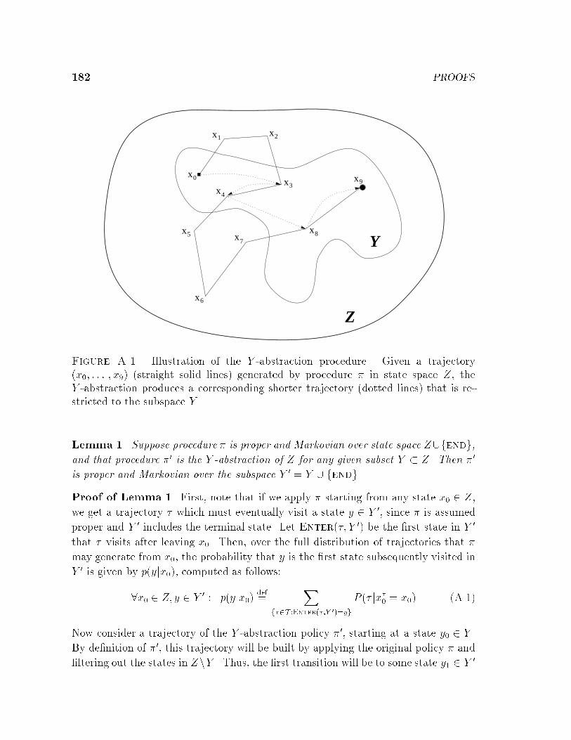
182 PROOFS
x2x1
x3x4
x5
x6
x7
x8
x9x0
Y
Z
Figure A.1. Illustration of the Y -abstraction procedure. Given a trajectory(x0; : : : ; x9) (straight solid lines) generated by procedure � in state space Z, theY -abstraction produces a corresponding shorter trajectory (dotted lines) that is re-stricted to the subspace Y .
Lemma 1. Suppose procedure � is proper and Markovian over state space Z[fendg,
and that procedure �0 is the Y -abstraction of Z for any given subset Y � Z. Then �0
is proper and Markovian over the subspace Y 0 = Y [ fendg.
Proof of Lemma 1. First, note that if we apply � starting from any state x0 2 Z,
we get a trajectory � which must eventually visit a state y 2 Y 0, since � is assumed
proper and Y 0 includes the terminal state. Let Enter(�; Y 0) be the �rst state in Y 0
that � visits after leaving x0. Then, over the full distribution of trajectories that �
may generate from x0, the probability that y is the �rst state subsequently visited in
Y 0 is given by p(yjx0), computed as follows:
8x0 2 Z; y 2 Y 0 : p(yjx0)def=
Xf�2T :Enter(�;Y 0)=yg
P (� jx�0 = x0) (A.1)
Now consider a trajectory of the Y -abstraction policy �0, starting at a state y0 2 Y .
By de�nition of �0, this trajectory will be built by applying the original policy � and
�ltering out the states in ZnY . Thus, the �rst transition will be to some state y1 2 Y 0
xA.1 THE BEST-SO-FAR PROCEDURE IS MARKOVIAN 183
with probability given precisely by p(y1jy0) as de�ned in Equation A.1. Furthermore,
by the Markov assumption on �, the future transitions from y1 will be independent
of the trajectory history and obey the same probabilities p(yi+1jyi) 8i � 0. Thus, �0
is Markovian over Y 0. �0 is also clearly proper, by inheritance from �.
I now �ll in the details of the proof of Proposition 2, following the three-part
outline sketched above.
Proof of Proposition 2.
1. In the statement of the proposition, �0 is de�ned to be the procedure that results
when patience-based termination is imposed on a procedure � that is Markovian,
but not necessarily proper. Recall that patience-based termination means, for
a given patience level Pat � 1, that any trajectory will end deterministically
as soon as Pat consecutive steps are taken with no improvement over the best
state found so far. That is, for all trajectories � produced by �0:
(t � Pat) ^ (x�t�Pat = minfj:0�j�tg
Obj(x�j )) ) x�t+1 = end:
Since the state space X is assumed �nite, �0 is certainly proper: the Obj val-
ues cannot keep decreasing forever. However, �0 is not necessarily Markovian.
Because of the new termination condition, the transition probability
P(x�i+1 = xi+1 j x�0 = x0; x
�1 = x1; : : : ; x
�i = xi)
is not independent of the history x0; : : : ; xi�1 as required by De�nition 3 (page 57).
In particular, the probability of termination depends not just on the current
state, but also on how recently the best-so-far state was found, and what the
Obj value at that state was.
However, the procedure �0 can be made Markovian by augmenting the state
space with these relevant extra variables. De�ne the augmented state space
Z = X �<� N, where the three components of a state z 2 Z are given by
a(z) 2 X; representing a state x in the original state space
b(z) 2 <; representing the best Obj value seen on the current trajectory
c(z) 2 N; representing the count of non-improving steps since �nding b(z).
In this augmented space, a trajectory of procedure �0 begins at the state z�0 =
hx�0;Obj(x�0); 0i. All future state transitions depend only on the current state

184 PROOFS
z�i . There are three kinds of possible transitions: (1) the patience counter may
expire, causing deterministic termination; (2) a new best-so-far state may be
discovered, in which case b(z) is updated and c(z) is reset to zero; or (3) an
ordinary transition to a non-best-so-far state occurs, in which case c(z) is simply
incremented. These give rise to the following Markovian transition probabilities:
8z 2 Z; z0 2 Z [ fendg,
P(z�i+1 = z0 j z�i = z) =8>>><>>>:1 if (c(z) = Pat) ^ (z0 = end)
p(a(z0)ja(z)) if (Obj(a(z0)) < b(z)) ^ (b(z0) = Obj(a(z0))) ^ (c(z0) = 0)
p(a(z0)ja(z)) if (Obj(a(z0)) � b(z)) ^ (b(z0) = b(z)) ^ (c(z0) = c(z) + 1)
0 otherwise.
Thus, �0 is proper and Markovian over the space Z [ fendg, concluding the
�rst segment of our proof.
2. We now apply Lemma 1 to show that the best-so-far abstraction of �0, denoted
bsf(�0), is also proper and Markovian in the augmented state space Z. Let the
subset Y be de�ned by
Y = fz 2 Z : (b(z) = Obj(a(z))) ^ (c(z) = 0)g:
Y consists of precisely the best-so-far states on any trajectory of �0. By Lemma 1,
bsf(�0) is proper and Markovian over the subspace Y [ fendg. That is, fol-
lowing procedure bsf(�0), the transitions from any state y are given by �xed
probabilities p(y0jy) independent of any past history of the procedure.
3. Finally, we note that every state y 2 Y has the form hx;Obj(x); 0i. All the
information about the state y is determined by the �rst component, the under-
lying state in the un-augmented space. It follows that the procedure bsf(�0)
is Markovian in the underlying space X [ fendg, with transition probabilities
given simply by
P(x�i+1 = x0 j x�i = x) = p(hx0;Obj(x0); 0i j hx;Obj(x); 0i):
We note that the property of strict monotonicity follows trivially from the de�nition
of bsf, completing the proof of Proposition 2.
xA.2 LEAST-SQUARES TD(1) IS EQUIVALENT TO LINEAR REGRESSION 185
A.2 Least-Squares TD(1) Is Equivalent to Linear Regression
This section demonstrates that the incremental algorithm LSTD(1), which is a special
case of the LSTD(�) procedure introduced in Section 6.1.2, produces an approximate
value function which is equivalent to that which would be generated by standard,
non-incremental, least-squares linear regression.
To be precise, assume we are given a sample trajectory (x0; x1; : : : ; xL;end) of a
Markov chain, with one-step rewards of R(xj; xj+1) on each step. From this trajectory,
a supervised learning system would generate the training pairs:
�0 7! R(x0; x1) +R(x1; x2) + � � �+R(xL;end)
�1 7! R(x1; x2) + � � � +R(xL;end)
... 7!...
�L 7! R(xL;end)
where �i is the vector of features representing state xi. Performing standard least-
squares linear regression on the above training set, as described for STAGE in Chap-
ter 3 (Equation 3.8, page 67), produces the following regression matrices:
ALR =LXi=0
�i�T
i bLR =LXi=0
�iyi
where yi =LXj=i
R(xj ; xj+1)
I now show that, thanks to the algebraic trick of the eligibility vectors zt, LSTD(1)
builds the equivalent A and b fully incrementally|without having to store the tra-
jectory while waiting to observe the eventual outcome yi. Please refer to Table 6.1.1
(p. 140) for the de�nition of the algorithm.
Proof. With simple algebraic manipulations, the sums built by LSTD(1)'s A and b
telescope neatly into ALR and bLR, as follows:
A =LXi=0
zt��i � �i+1
�T
=LXi=0
� iXj=0
�j
�(�i � �i+1)
T (by de�nition of zt)
=LXi=0
iXj=0
�j�T
i �LXi=0
iXj=0
�j�T
i+1

186 PROOFS
=��0�
T
0 +LXi=1
iXj=0
�j�T
i
���L+1Xk=1
k�1Xj=0
�j�T
k
�(substituting k � i+ 1)
= �0�T
0 +LXi=1
iXj=0
�j�T
i �LXk=1
k�1Xj=0
�j�T
k (since �L+1def= 0)
= �0�T
0 +LXi=1
� iXj=0
�j�T
i �i�1Xj=0
�j�T
i
�(substituting i � k)
=
LXi=0
�i�T
i
= ALR; as desired;
and
b =LXi=0
ziR(xi; xi+1)
=LXi=0
� iXj=0
�j
�R(xi; xi+1) (by de�nition of zt)
=
LXi=0
LXj=0
1(j � i)�jR(xi; xi+1) (where 1(True)def= 1, 1(False)
def= 0)
=LXj=0
LXi=0
1(j � i)�jR(xi; xi+1)
=LXj=0
�j
LXi=j
R(xi; xi+1)
= bLR; as desired.
These reductions prove that the contributions to A and b by any single trajectory
are identical in LSTD(1) and least-squares linear regression. In both algorithms,
contributions from multiple trajectories are simply summed into the matrices. Thus,
LSTD(1) and linear regression compute the same statistics and, ultimately, the same
coe�cients for the approximated value function.

187
Appendix B
Simulated Annealing
B.1 Annealing Schedules
Simulated annealing (SA) is described by the template in Table B.1. The main imple-
mentation challenge is to choose an e�ective annealing schedule for the temperature
parameter. The temperature ti controls the probability of accepting a step to a worse
neighbor: when ti = +1, SA accepts any step, acting as a random walk; whereas
when ti = 0, SA rejects all worsening steps, acting as stochastic hillclimbing with
equi-cost moves.
Simulated-Annealing(X, S, N , Obj, TotEvals, Schedule):Given:� a state space X� starting states S � X� a neighborhood structure N : X ! 2X
� an objective function, Obj : X ! <, to be minimized� TotEvals, the number of state evaluations allotted for this run� an annealing Schedule which determines the temperature on each iteration
1. Let x0 2 S be a random starting state for search;let t0 := the initial temperature of Schedule
2. For i := 0 to TotEvals� 1, do:
(a) Choose x0 := a random element from N(xi)
(b) xi+1 :=
(x0 if rand[0,1) < e[Obj(xi)�Obj(x
0)]=ti
xi otherwise
(c) Update temperature ti+1 according to Schedule
3. Return the best state found.
Table B.1. A template for the simulated annealing algorithm
The temperature annealing schedule has been the subject of extensive theoreti-
188 SIMULATED ANNEALING
cal and experimental analysis in the simulated annealing literature [Boese 96]. The
possibilities include the following:
� Logarithmic: ti = = log(i+ 2). For su�ciently high , a schedule of this form
guarantees that SA will converge with probability one to the globally optimal
solution [Mitra et al. 86,Hajek 88]. Unfortunately, this guarantee only applies
in the limit as TotEvals!1. Logarithmic schedules are generally too slow
for practical use.
� Geometric: for a �xed initial temperature t0, cooling rate � 2 (0; 1) and round
length L � 1, de�ne ti = t0 � �bi=Lc. This is the original schedule proposed by
Kirkpatrick [83], and is still widely used in practice [Johnson et al. 89,Johnson
et al. 91,Press et al. 92]. However, the parameters t0, L, and � must be tuned
for each problem instance.
� Adaptive: a variety of adaptive schedules have been proposed, with both the-
oretical and practical motivations. [Boese 96] summarizes the most notable of
these, including the schedules of [Aarts and van Laarhoven 85], [Huang et al. 86],
and [Lam and Delosme 88]. According to [Ochotta 94],
Results for the Lam schedule are quite impressive. When compared
with other general-purpose annealing schedules such as [Huang et
al. 86] and even hand-crafted schedules like the one in [Sechen and
Sangiovanni-Vincentelli 86], it often provides speed-ups of 50% while
actually improving the quality of the �nal answers [Lam and Delosme
88]. Simulated annealing with the Lam schedule even compares fa-
vorably with heuristic combinatorial optimization methods tuned to
speci�c problems like partitioning and the travelling salesman prob-
lem [Lam 88].
B.2 The \Modi�ed Lam" Schedule
For the purposes of comparing against STAGE, I sought to implement simulated an-
nealing with a cooling schedule which would both perform very well and would require
little tuning from one problem instance to the next. After some experimentation, I
settled on an adaptive schedule similar to that used in [Ochotta 94], which in turn was
based on Swartz's modi�cation of the Lam schedule [Swartz and Sechen 90]. Swartz
observed that for each of a large number of annealing runs using the Lam schedule,
the accept ratio|that is, the ratio of moves accepted to moves considered|followed
an almost identical pattern with respect to the move counter i [Ochotta 94, p. 137]:

xB.2 THE \MODIFIED LAM" SCHEDULE 189
The accept rate starts at about 100%, decreases exponentially until it sta-
bilizes (about 15% of the way through the run) at about 44%, and remains
there until about 65% of the way through the run. It then continues its
exponential decline until the end of the annealing process. Based on this
observation, Swartz duplicated the e�ect of the Lam schedule by using a
simple feedback loop to control the temperature and force the accept ratio
to follow the curve in Figure [B.1]. In comparing the modi�ed schedule to
the original schedule, Swartz reported almost no di�erence in the quality
of the �nal answers [Swartz and Sechen 90]. One additional bene�t of the
modi�ed Lam schedule is that, in contrast to the original schedule, the
total number of moves in the annealing run can be speci�ed by the user.
0
0.1
0.2
0.3
0.4
0.5
0.6
0.7
0.8
0.9
1
0 0.2 0.4 0.6 0.8 1
targ
et a
ccep
t rat
io
percentage of moves completed
Figure B.1. Accept rate targets for the modi�ed Lam schedule
All details of my implementation of Swartz's modi�ed Lam schedule are given
below in Table B.2. I do not dynamically readjust the neighborhood structure N(x)
over the course of search, as the original Lam schedule did, since such readjustments
cannot be speci�ed in a problem-independent manner.

190 SIMULATED ANNEALING
Simulated-Annealing(X, S, N , Obj, TotEvals,Modi�ed-Lam-Schedule):
1. Let x0 2 S be a random starting state for search;let AcceptRate:=0.5, t0 := 0:5.
2. For i := 0 to TotEvals� 1, do:
(a) Choose x0 := a random element from N(xi)
(b) xi+1 :=
(x0 if rand[0,1) < e[Obj(xi)�Obj(x
0)]=ti
xi otherwise
(c) Update temperature ti+1 as follows:
i. let AcceptRate :=
(1500(499 �AcceptRate+ 1) if x0 was accepted1500(499 �AcceptRate) if x0 was rejected
ii. let d := i=TotEvals
iii. let TargRate :=
8><>:0:44 + 0:56 � 560�d=0:15 if 0 � d < 0:15
0:44 if 0:15 � d < 0:65
0:44 � 440�(d�0:65)=0:35 if 0:65 � d < 1
iv. let ti+1 :=
(ti � 0:999 if AcceptRate > TargRate
ti=0:999 otherwise
3. Return the best state found.
Table B.2. Details of the \modi�ed Lam" adaptive simulated annealing schedule,instantiating the template of Figure B.1. The TargRate function is plotted inFigure B.1.

xB.3 EXPERIMENTS 191
B.3 Experiments
I certainly do not claim that the modi�ed Lam schedule is perfectly optimized for
every problem attempted in Chapter 4. Getting the best performance from simu-
lated annealing on any given problem is an art that involves re�ning the temperature
schedule, dynamically adjusting the search neighborhood, and tuning the cost func-
tion coe�cients. However, empirically, the simulated annealing algorithm de�ned by
Table B.2 does seem to perform very well on a wide variety of problems without
requiring further tuning.
The following experiments illustrate the e�ectiveness of my implementation. I
consider four of the optimization domains of Chapter 4: bin-packing (x4.2), VLSI
channel routing (x4.3), Bayes net learning (x4.4), and cartogram design (x4.6). For
each of these domains, I compare the performance of the modi�ed Lam schedule
with that of 12 di�erent geometric cooling schedules, de�ned by ti = t0 � �i for all
combinations of
initial temperature t0 2 f10; 1; 0:1; 0:01g
cooling rate � 2 f0:9999; 0:99999; 0:999999g:
The total length of the schedules is set to TotEvals, the same setting used in the
comparative experiments of Chapter 4: 105 for bin-packing and Bayes net learning,
5 � 105 for channel routing, and 106 for cartogram design.
Results are shown in Figures B.2{B.5. Each �gure plots thirteen boxes: the left-
most box corresponds to the modi�ed Lam schedule results (copied from Chapter 4),
and the other 12 boxes correspond to the performance of the various geometric cool-
ing schedules (averaged over 10 runs each). In all cases, the modi�ed Lam schedule is
nearly as e�ective as, if not more e�ective than, the best of the geometric schedules.

192 SIMULATED ANNEALING
105
110
115
120
125
Lam geo1 geo2 geo3 geo4 geo5 geo6 geo7 geo8 geo9 geo10 geo11 geo12
Num
ber
of b
ins
(103
is o
ptim
al)
Figure B.2. Simulated annealing schedules for bin-packing instance u250 13: Mod-i�ed Lam schedule (leftmost) versus 12 geometric cooling schedules
10
15
20
25
30
35
40
45
50
Lam geo1 geo2 geo3 geo4 geo5 geo6 geo7 geo8 geo9 geo10 geo11 geo12
Are
a of
circ
uit l
ayou
t (10
is o
ptim
al)
Figure B.3. Simulated annealing schedules for channel routing instance YK4: Mod-i�ed Lam schedule (leftmost) versus 12 geometric cooling schedules

xB.3 EXPERIMENTS 193
750000
800000
850000
900000
950000
1e+06
Lam geo1 geo2 geo3 geo4 geo5 geo6 geo7 geo8 geo9 geo10 geo11 geo12
Bay
es n
et s
core
Figure B.4. Simulated annealing schedules for Bayes net structure-�nding instanceSYNTH125K: Modi�ed Lam schedule (leftmost) versus 12 geometric cooling schedules
0
0.1
0.2
0.3
0.4
0.5
Lam geo1 geo2 geo3 geo4 geo5 geo6 geo7 geo8 geo9 geo10 geo11 geo12
Map
err
or fu
nctio
n
Figure B.5. Simulated annealing schedules for cartogram design instance US49:Modi�ed Lam schedule (leftmost) versus 12 geometric cooling schedules

194
195
Appendix C
Implementation Details of Problem Instances
This appendix gives implementation details for the optimization problems used in the
experiments of Chapter 4. For further information, including the complete datasets
used in the bin-packing, Bayes net structure-�nding, and cartogram domains, please
access the following web page:
http://www.cs.cmu.edu/~AUTON/stage/ (C.1)
C.1 Bin-packing
The bin-packing problem was introduced in Sections 3.3.2 and 4.2. We are given a bin
capacity C and a list L = (a1; a2; :::an) of items, each having a size s(ai) > 0. The goal
is to pack the items into as few bins as possible, i.e., partition them into a minimum
number m of subsets B1; B2; :::; Bm such that for each Bj ,P
ai2Bjs(ai) � C.
In the STAGE experiments, value function approximation was done with respect
to two state features: the objective function itself, and the variance in bin fullness
levels. In terms of the above notation, given a packing x = fB1; B2; : : : ; BMxg (with
all bins Bj assumed non-empty), we have
Obj(x)def= Mx
Var(x)def=
1
Mx
MxXj=1
fullness(Bj)2
!�
1
Mx � C
nXi=1
s(ai)
!2
where
fullness(Bj)def=
1
C
Xai2Bj
s(ai) :
The illustrative example of Section 3.3.2 consisted of the following 30 items, to be
packed into bins of capacity 100:
(27, 23, 23, 23, 27, 26, 26, 51, 26, 23,51, 23, 51, 23, 23, 51, 23, 23, 27, 23,51, 27, 51, 26, 27, 23, 26, 27, 26, 23)

196 IMPLEMENTATION DETAILS OF PROBLEM INSTANCES
These particular item sizes were motivated by Figure 2.5 of [Co�man et al. 96], which
depicts a template of a worst-case example for the \First Fit Decreasing" o�ine bin-
packing heuristic. The optimal packing �lls 9 bins exactly to capacity.
The twenty instances of the u250 class were contributed to the Operations Re-
search Library by Falkenauer [96]. They may be downloaded from the web page
referenced at the start of this section, or directly from the OR-Library web site at
http://www.ms.ic.ac.uk/info.html :
C.2 VLSI Channel Routing
My implementation of channel routing follows that of the SACR system [Wong et
al. 88]. This system allows a restricted form of doglegging, whereby a net may be
split horizontally only at columns containing a pin belonging to that net.
Most of the experiments in this dissertation were conducted on the instance YK4.
That instance is speci�ed by the following pin columns:
Upper: 17 9 23 33 0 17 34 33 32 31 32 20 9 10 21 34 0 31 22 10 0 22 1 3 16 0 0 0 9
19 7 0 16 14 7 51 43 57 67 0 51 68 67 66 65 66 54 43 44 55 68 0 65 56 44 0 56
35 37 50 0 0 0 43 53 41 0 50 48 41 85 77 91 101 0 85 102 101 100 99 100 88 77
78 89 102 0 99 90 78 0 90 69 71 84 0 0 0 77 87 75 0 84 82 75 119 111 125 135 0
119 136 135 134 133 134 122 111 112 123 136 0 133 124 112 0 124 103 105 118
0 0 0 111 121 109 0 118 116 109
Lower: 0 0 0 24 10 0 4 2 21 2 4 23 1 4 24 1 4 2 0 1 4 0 3 19 2 3 20 2 3 14 3 1 9 24 0
0 0 0 58 44 0 38 36 55 36 38 57 35 38 58 35 38 36 0 35 38 0 37 53 36 37 54 36
37 48 37 35 43 58 0 0 0 0 92 78 0 72 70 89 70 72 91 69 72 92 69 72 70 0 69 72 0
71 87 70 71 88 70 71 82 71 69 77 92 0 0 0 0 126 112 0 106 104 123 104 106 125
103 106 126 103 106 104 0 103 106 0 105 121 104 105 122 104 105 116 105 103
111 126 0
These pin columns correspond to Example 1 (Figure 25) of [Yoshimura and Kuh
82], but multiplied four times and placed side by side. By \cloning" the problem in
this manner, we maintain the known global optimum (in this case, 10 tracks when
restricted doglegging is allowed), but make the problem much more di�cult for local
search.
In Section 6.2, I applied STAGE to eight additional channel routing instances,
HYC1 through HYC8. The pin columns for these problems may be found in [Chao
and Harper 96] and are also available on the STAGE web page.

xC.3 BAYES NETWORK LEARNING 197
C.3 Bayes Network Learning
For the experimentswith the Bayes-net structure-�nding domain (Sections 4.4 and 6.1.5),
three datasets were used: MPG, ADULT2, and SYNTH125K.
� The MPG dataset contains information on the horsepower, weight, gas mileage,
and other such data (10 total attributes) for 392 automobiles. It is derived from
the \Auto-Mpg" dataset available from the UCI Machine Learning repository
[Merz and Murphy 98], but modi�ed by coarsely discretizing all continuous
variables.
� The ADULT2 dataset was also obtained from the UCI repository. It consists of
census data related to the job, wealth, nationality, etc. (15 total attributes) on
30,162 individuals.
� The SYNTH125K dataset was generated synthetically from the probability dis-
tribution given by the Bayes net in Figure 4.7 (p. 86), designed by Moore and
Lee [98].
All three datasets are available for downloading from the STAGE web page.
C.4 Radiotherapy Treatment Planning
The radiotherapy treatment planning domain of Section 4.5 is too complex to explain
in full detail here. Please refer to the web page for more information. Here, I describe
the domain in enough detail to illustrate its complexity|in particular, to show why
we must resort to using local search rather than, say, linear programming to solve
it. The form of my objective function was based on discussions with domain experts;
however, I did not have access to a medically accurate implementation of the dose
calculations and penalty functions. Thus, I claim only that the optimization problem
solved here retains most of the overall structure and geometry of tradeo�s found in
the true medical domain.
I formulated the problem as follows. The treatment area is discretized into an
80 � 80 rectangular grid. The radiation dosage dosep(x) at each pixel p can then
be calculated from the current plan x according to a known forward model. Pixels
within the area of the tumor t have a target dose targt and incur a penalty based on
the ratio rp =dosep(x)targt
:
Penalty(p) =
(exp(1=max(rp; 0:1)) if rp < 1 (underdose)
rp � 1 if rp � 1 (overdose)
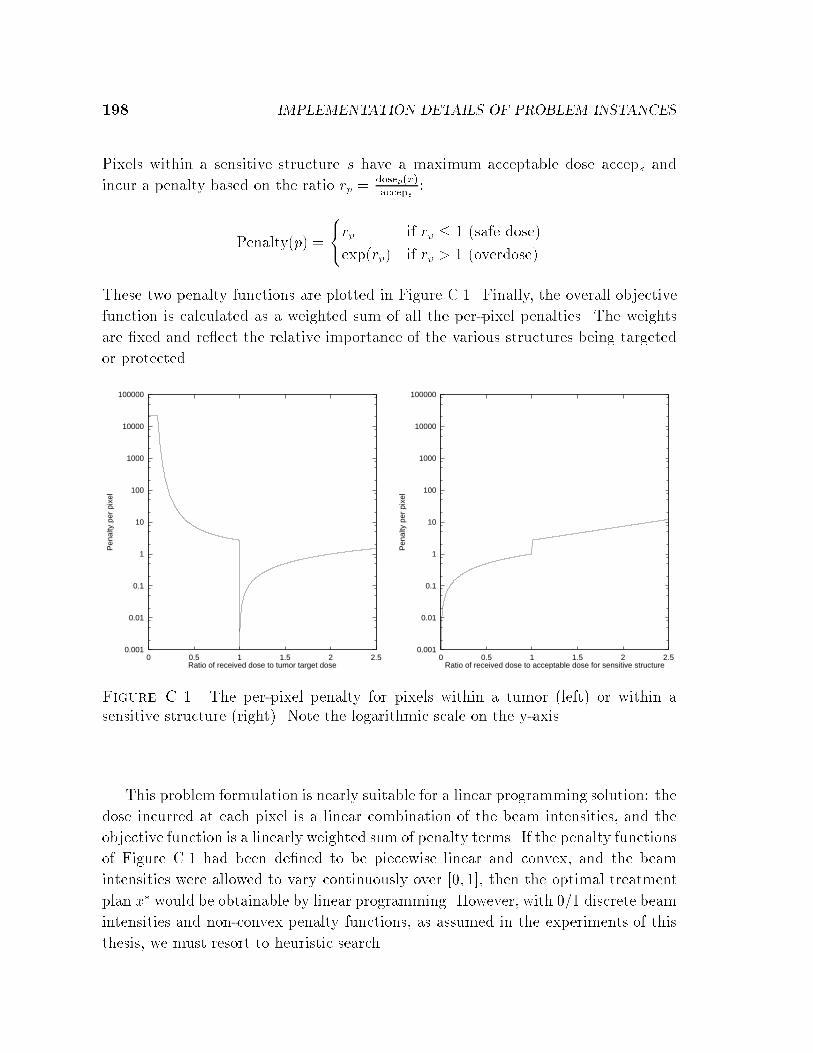
198 IMPLEMENTATION DETAILS OF PROBLEM INSTANCES
Pixels within a sensitive structure s have a maximum acceptable dose acceps and
incur a penalty based on the ratio rp =dosep(x)acceps
:
Penalty(p) =
(rp if rp � 1 (safe dose)
exp(rp) if rp > 1 (overdose)
These two penalty functions are plotted in Figure C.1. Finally, the overall objective
function is calculated as a weighted sum of all the per-pixel penalties. The weights
are �xed and re ect the relative importance of the various structures being targeted
or protected.
0.001
0.01
0.1
1
10
100
1000
10000
100000
0 0.5 1 1.5 2 2.5
Pen
alty
per
pix
el
Ratio of received dose to tumor target dose
0.001
0.01
0.1
1
10
100
1000
10000
100000
0 0.5 1 1.5 2 2.5
Pen
alty
per
pix
el
Ratio of received dose to acceptable dose for sensitive structure
Figure C.1. The per-pixel penalty for pixels within a tumor (left) or within asensitive structure (right). Note the logarithmic scale on the y-axis.
This problem formulation is nearly suitable for a linear programming solution: the
dose incurred at each pixel is a linear combination of the beam intensities, and the
objective function is a linearly weighted sum of penalty terms. If the penalty functions
of Figure C.1 had been de�ned to be piecewise linear and convex, and the beam
intensities were allowed to vary continuously over [0; 1], then the optimal treatment
plan x� would be obtainable by linear programming. However, with 0/1 discrete beam
intensities and non-convex penalty functions, as assumed in the experiments of this
thesis, we must resort to heuristic search.

xC.5 CARTOGRAM DESIGN 199
C.5 Cartogram Design
The cartogram design problem was introduced in Section 4.6. This thesis investigated
a single instance, US49. Instance US49 is de�ned by the 49 polygons of the continental
U.S. map (48 states plus the District of Columbia) and their respective target areas,
which are based on the 1990{2000 electoral vote for U.S. President. This dataset is
available from the STAGE web page.
Local search moves in this domain consist of choosing one of the 162 points and
perturbing it slightly. These points are chosen randomly, but with a bias toward
those points that contribute most to the current map error function. To be precise:
�rst a state is chosen with probability proportional to its contribution to Obj(x), and
then one point on that state is chosen uniformly at random. The perturbation is then
generated by adding uniformly random numbers in [�1:5; 1:5] to each coordinate.
The objective function is de�ned as the sum of four penalty terms:
Obj(x) = �Area(x) + �Gape(x) + �Orient(x) + �Segfrac(x)
The penalty terms are de�ned as follows:
�Area(x) =10
#States
Xs2States
�max
� Areax(s)
Areatarg(s);
Areatarg(s)
max(Areax(s); 0:001)
�� 1�2
�Gape(x) =1
#Bends
X\ABC2Bends
�measurex(\ABC)�measureorig(\ABC)
�2�Orient(x) =
1
#Bends
X\ABC2Bends
�measurex(\AB )�measureorig(\AB )
�2�Segfrac(x) =
10
#Bends
X\ABC2Bends
� lengthx(AB)
perimx(State(\ABC))�
lengthorig(AB)
perimorig(State(\ABC))
�2The \Bends" above index each angle of each polygon in the map. The notation
\\AB " refers to the angle made between line$
AB and the x-axis (a �xed horizontal
line). Finally, the constants 1 and 10 in these penalty terms were chosen by trial and
error to create aesthetically appealing cartograms.
C.6 Boolean Satis�ability
The di�cult \32-bit parity function learning" instances tested in Section 4.7 are
described in [Crawford 93]. The complete formulas are available for downloading
from the STAGE web page, and also from the DIMACS satis�ability archive:
ftp://dimacs.rutgers.edu/pub/challenge/sat/benchmarks/cnf/ :

200
201
References
E. H. L. Aarts and P. J. M. van Laarhoven. A new polynomial-time cooling schedule.In Proc. IEEE Intl. Conf. on Computer-Aided Design, pages 206{208, 1985. (p. 188)
B. Abramson. Expected-outcome: A general model of static evaluation. IEEETransactions on Pattern Analysis and Machine Intelligence, 12(2):182{193, February1990. (pp. 167, 168)
D. H. Ackley and M. L. Littman. A case for distributed Lamarckian evolution. InC. Langton, C. Taylor, J. D. Farmer, and S. Ramussen, editors, Arti�cial Life III:Santa Fe Institute Studies in the Sciences of Complexity, volume 10, pages 487{509.Addison-Wesley, Redwood City, CA, 1993. (p. 170)
J. S. Albus. Brains, Behavior, and Robotics. Byte Books, Peterborough, NH, 1981.(p. 65)
D. Aldous and U. Vazirani. \Go with the winners" algorithms. In Proceedings of the35th Symposium on Foundations of Computer Science, pages 492{501, 1994. (p. 162)
D. Applegate, R. Bixby, V. Chvatal, and B. Cook. Finding cuts in the TSP (Apreliminary report). Technical Report 95-05, DIMACS, April 10, 1995. (p. 42)
C. G. Atkeson and J. C. Santamaria. A comparison of direct and model-basedreinforcement learning. In International Conference on Robotics and Automation,1997. (p. 145)
C. G. Atkeson. Using local trajectory optimizers to speed up global optimizationin dynamic programming. In J. D. Cowan, G. Tesauro, and J. Alspector, editors,Advances in Neural Information Processing Systems 6. Morgan Kaufmann, 1994.(p. 25)
L. Baird. Residual algorithms: Reinforcement learning with function approximation.In Machine Learning: Proceedings of the Twelfth International Conference, 1995.(pp. 13, 23)
S. Baluja and R. Caruana. Removing the genetics from the standard genetic algo-rithm. In Proc. 12th International Conference on Machine Learning, pages 38{46.Morgan Kaufmann, 1995. (p. 170)
S. Baluja and S. Davies. Combining multiple optimization runs with optimal depen-dency trees. Technical Report CMU-CS-97-157, Carnegie Mellon University Schoolof Computer Science, 1997. (pp. 74, 170)
202
R. S. Barr, B. L. Golden, J. P. Kelly, M. G. C. Resende, and W. R. Stewart. Design-ing and reporting on computational experiments with heuristic methods. Journal ofHeuristics, 1(1):9{32, 1995. (pp. 70, 72)
A. Barto, R. Sutton, and C. Watkins. Learning and sequential decision making.Technical Report COINS 89-95, University of Massachusetts, 1989. (p. 20)
A. G. Barto, S. J. Bradtke, and S. P. Singh. Real-time learning and control usingasynchronous dynamic programming. Arti�cial Intelligence, 1995. (pp. 20, 21)
J. Baxter, A. Tridgell, and L. Weaver. KnightCap: A chess program that learns bycombining TD(�) with minimax search. Technical report, Department of SystemsEngineering, Australian National University, Canberra, Australia, November 1997.(p. 168)
R. Bellman, R. Kalaba, and B. Kotkin. Polynomial approximation|a new compu-tational technique in dynamic programming: Allocation processes. Mathematics OfComputation, 17, 1963. (p. 20)
R. Bellman. Dynamic Programming. Princeton University Press, 1957. (pp. 13, 19)
R. Bellman. An Introduction to Arti�cial Intelligence: Can Computers Think? Boyd& Fraser Publishing Company, 1978. (p. 20)
D. A. Berry and B. Fristedt. Bandit Problems: Sequential Allocation of Experiments.Chapman and Hall, 1985. (p. 32)
D. Bertsekas and J. Tsitsiklis. Neuro-Dynamic Programming. Athena Scienti�c,Belmont, MA, 1996. (pp. 13, 19, 20, 21, 23, 24, 64, 66, 137, 138, 139, 141, 142, 143, 150)
D. Bertsekas, J. Tsitsiklis, and C. Wu. Rollout algorithms for combinatorial op-timization. Technical Report LIDS-P 2386, MIT Laboratory for Information andDecision Systems, 1997. (p. 167)
D. Bertsekas. A counterexample to temporal di�erences learning. Neural Computa-tion, 7:270{9, 1995. (p. 13)
J.R. Beveridge, C. Graves, and C. E. Lesher. Local search as a tool for horizon linematching. Technical Report CS-96-109, Colorado State University, 1996. (pp. 41, 70,161)
K. D. Boese, A. B. Kahng, and S. Muddu. A new adaptive multi-start technique forcombinatorial global optimizations. Operations Research Letters, 16:101{113, 1994.(pp. 162, 163, 170)
203
K. D. Boese. Cost versus distance in the traveling salesman problem. TechnicalReport CSD-950018, UCLA Computer Science Department, May 1995. (pp. 162,
163)
K. D. Boese. Models for Iterative Global Optimization. PhD thesis, UCLA ComputerScience Department, 1996. (pp. 162, 188)
J. A. Boyan and A. W. Moore. Generalization in reinforcement learning: Safelyapproximating the value function. In G. Tesauro, D. S. Touretzky, and T. K. Leen,editors, Advances In Neural Information Processing Systems 7. MIT Press, 1995.(pp. 13, 14, 23, 25, 27)
J. A. Boyan and A. W. Moore. Learning evaluation functions for large acyclicdomains. In L. Saitta, editor, Machine Learning: Proceedings of the ThirteenthInternational Conference. Morgan Kaufmann, 1996. (pp. 14, 25)
J. A. Boyan and A. W. Moore. Using prediction to improve combinatorial opti-mization search. In Proceedings of the Sixth International Workshop on Arti�cialIntelligence and Statistics (AISTATS), January 1997. (p. 14)
J. A. Boyan and A. W. Moore. Learning evaluation functions for global optimizationand Boolean satis�ability. In Proceedings of the Fifteenth National Conference onArti�cial Intelligence (AAAI), 1998. (Outstanding Paper Award). (p. 14)
J. A. Boyan, A. W. Moore, and R. S. Sutton, editors. Proceedings of the Workshopon Value Function Approximation, Machine Learning Conference, July 1995. CMU-CS-95-206. Internet resource available at http://www.cs.cmu.edu/~reinf/ml95/.(pp. 13, 19)
J. A. Boyan, D. Freitag, and T. Joachims. A machine learning architecture foroptimizing web search engines. Technical Report AAAI Technical Report WS-96-06,Proceedings of the AAAI workshop on Internet-Based Information Systems, 1996.(p. 41)
J. A. Boyan. Modular neural networks for learning context-dependent game strate-gies. Master's thesis, University of Cambridge, Department of Engineering andComputer Laboratory, 1992. (pp. 13, 21, 168)
S. J. Bradtke and A. G. Barto. Linear least-squares algorithms for temporal di�er-ence learning. Machine Learning, 22(1/2/3):33{57, 1996. (pp. 15, 137, 143, 175)
L. Breiman, J. H. Friedman, R. A. Olshen, and C. J. Stone. Classi�cation andregression trees. Technical report, Wadsworth International, Monterey, CA, 1984.(p. 65)
204
W. L. Buntine, L. Su, R. Newton, and A. Mayer. Adaptive methods for netlistpartitioning. In Proceedings of ICCAD-97, San Jose, CA, November 1997. (p. 167)
M. S. Campbell. Deep Blue: The IBM chess machine. Talk given at Carnegie MellonUniversity, March 1998. (p. 12)
Y. Censor, M. D. Altschuler, and W. D. Powlis. A computational solution of theinverse problem in radiation-therapy treatment planning. Applied Mathematics andComputation, 25:57{87, 1988. (pp. 90, 91)
H-Y. Chao and M. P. Harper. An e�cient lower bound algorithm for channel routing.Integration: The VLSI Journal, 1996. (pp. 79, 154, 196)
D. M. Chickering, D. Geiger, and D. Heckerman. Learning bayesian networks isNP-hard. Technical Report MSR-TR-94-17, Microsoft Research, November 1994.(pp. 84, 85)
J. Christensen and R. Korf. A uni�ed theory of heuristic evaluation functions and itsapplication to learning. In Proceedings of the 4th National Conference on Arti�cialIntelligence, pages 148{152, 1986. (p. 20)
J. Christensen. Learning static evaluation functions by linear regression. InT. Mitchell, J. Carbonell, and R. Michalski, editors, Machine learning: A guideto current research, pages 39{42. Kluwer, Boston, 1986. (pp. 20, 168)
W. S. Cleveland and S. J. Devlin. Locally weighted regression: An approach toregression analysis by local �tting. Journal of the American Statistical Association,83(403):596{610, September 1988. (pp. 38, 65)
E. G. Co�man, M. R. Garey, and D. S. Johnson. Approximation algorithms for binpacking: a survey. In D. Hochbaum, editor, Approximation Algorithms for NP-HardProblems. PWS Publishing, 1996. (pp. 42, 43, 76, 196)
J. M. Cohn. Automatic Device Placement for Analog Cells in KOAN. PhD thesis,Carnegie Mellon University Department of Electrical and Computer Engineering,February 1992. (pp. 47, 178)
T. H. Cormen, C. E. Leiserson, and R. L. Rivest. Introduction to Algorithms. MITPress, 1990. (p. 24)
J. Crawford. Propositional versions of parity learning problems. Internet resourceavailable by anonymous FTP, at ftp://dimacs.rutgers.edu/pub/challenge/-
sat/contributed/crawford/README, July 1993. (pp. 96, 199)
205
R. Crites and A. Barto. Improving elevator performance using reinforcement learn-ing. In D. Touretzky, M. Mozer, and M. Hasselmo, editors, Advances in NeuralInformation Processing Systems 8, 1996. (pp. 13, 21)
S. Davies and S. Baluja. Personal communication, April 1998. (p. 171)
J. S. de Bonet, C. L. Isbell Jr., and P. Viola. MIMIC: Finding optima by estimatingprobability densities. In Michael C. Mozer, Michael I. Jordan, and Thomas Petsche,editors, Advances in Neural Information Processing Systems, volume 9, page 424.The MIT Press, 1997. (p. 170)
R. Dearden, N. Friedman, and S. Russell. Bayesian Q-Learning. In Proceedings ofthe Fifteenth National Conference on Arti�cial Intelligence (AAAI), 1998. (p. 130)
F. D'Epenoux. A probabilistic production and inventory problem. ManagementScience, 10:98{108, 1963. (p. 19)
D. N. Deutsch. A `dogleg' channel router. In Proceedings of the 13th ACM/IEEEDesign Automation Conference, pages 425{433, 1976. (p. 79)
J. Doran and D. Michie. Experiments with the graph traverser program. Proceedingsof the Royal Society of London, 294, Series A:235{259, 1966. (p. 169)
M. Dorigo and L. Gambardella. Ant-Q: A reinforcement learning approach to combi-natorial optimization. Technical Report 95-01, Irdia, Universit�e Libre de Bruxelles,1995. (p. 167)
D. Dorling. Cartograms for visualizing human geography. In H. M. Hearnshawand D. J. Unwin, editors, Visualization in Geographical Information Systems, pages85{102. Wiley, 1994. (p. 93)
D. Dorling. Area cartograms: their use and creation. Number 59 in Conceptsand Techniques in Modern Geography. University of East Anglia: EnvironmentalPublications, 1996. (p. 93)
Q. Duan, S. Sorooshian, and V. Gupta. E�ective and e�cient global optimizationof conceptual rainfall-runo� models. Water Resources Research, 28(4):1015{1031,1992. (p. 41)
S. Fahlman and C. Lebiere. The Cascade-Correlation learning architecture. InD. Touretzky, editor, Advances in Neural Information Processing Systems 2. MorganKaufmann, 1990. (p. 65)
E. Falkenauer and A. Delchambre. A genetic algorithm for bin packing and linebalancing. In Proc. of the IEEE 1992 International Conference on Robotics andAutomation, pages 1186{1192, Nice, France, May 1992. (pp. 47, 74)

206
E. Falkenauer. A hybrid grouping genetic algorithm for bin packing. Journal ofHeuristics, 2(1):5{30, 1996. (pp. 74, 76, 77, 196)
N. Friedman and Z. Yakhini. On the sample complexity of learning Bayesian net-works. In Proc. 12th Conference on Uncertainty in Arti�cial Intelligence, 1996.(p. 84)
J. H. Friedman. Multivariate adaptive regression splines. Annals of Statistics,19(1):1{67, 1991. (p. 65)
N. Friedman. Learning belief networks in the presence of missing values and hiddenvariables. In Proc. 14th International Conference on Machine Learning, pages 125{133. Morgan Kaufmann, 1997. (pp. 84, 85)
M. R. Garey and D. S. Johnson. Computers and Intractability: A Guide to theTheory of NP-Completeness. Freeman, 1979. (pp. 42, 72, 95)
F. Glover and M. Laguna. Tabu search. In Modern Heuristic Techniques for Com-binatorial Problems. Scienti�c Publications, Oxford, 1993. (p. 164)
D. E. Goldberg. Genetic Algorithms in Search, Optimization, and Machine Learning.Addison-Wesley, Reading, Mass., 1989. (p. 169)
G. Gordon. Stable function approximation in dynamic programming. In Proceedingsof the 12th International Conference on Machine Learning. Morgan Kaufmann, 1995.(pp. 13, 23, 27)
S. M. Gusein-Zade and V. S. Tikunov. A new technique for constructing continu-ous cartograms. Cartography and Geographic Information Systems, 20(3):167{173,1993. (p. 93)
L. W. Hagen and A. B. Kahng. Combining problem reduction and adaptive multi-start: A new technique for superior iterative partitioning. IEEE Transactions onCAD, 16(7):709{717, 1997. (p. 164)
B. Hajek. Cooling schedules for optimal annealing. Math. Oper. Res., 13(2):311{329,1988. (p. 188)
M. Harmon, L. Baird, and A. H. Klopf. Advantage updating applied to a di�erentialgame. In G. Tesauro, D. S. Touretzky, and T. K. Leen, editors, Advances In NeuralInformation Processing Systems 7. MIT Press, 1995. (p. 18)
D. Heckerman, D. Geiger, and M. Chickering. Learning Bayesian networks: Thecombination of knowledge and statistical data. Technical Report MSR-TR-94-09,Microsoft Research, 1994. (pp. 84, 85)

207
G. E. Hinton and S. J. Nowlan. How learning can guide evolution. Complex Systems,1(1):495{502, June 1987. (p. 170)
R. Howard. Dynamic Programming and Markov Processes. MIT Press and JohnWiley & Sons, 1960. (pp. 19, 167)
F. Hsu, T. S. Anantharaman, M. S. Campbell, and A. Nowatzyk. A grandmasterchess machine. Scienti�c American, 263(4):44{50, October 1990. (p. 12)
M. D. Huang, F. Romeo, and A. Sangiovanni-Vincentelli. An e�cient general coolingschedule for simulated annealing. In Proceedings of the International Conference onComputer-Aided Design, pages 381{384, November 1986. (p. 188)
A. Jagota, L. Sanchis, and R. Ganesan. Approximating maximumclique using neuralnetwork and related heuristics. In D. S. Johnson and M. A. Trick, editors, DIMACSSeries: Second DIMACS Challenge. American Mathematical Society, 1996. (p. 164)
A. Jagota. An adaptive, multiple restarts neural network algorithm for graph color-ing. European J. of Oper. Res., 93:257{270, 1996. (p. 164)
Y. Jiang, H. Kautz, and B. Selman. Solving problems with hard and soft constraintsusing a stochastic algorithm for MAX-SAT. In First International Joint Workshop onArti�cial Intelligence and Operations Research, Timberline, Oregon, 1995. (p. 102)
D. S. Johnson and L. A. McGeoch. The traveling salesman problem: A case studyin local optimization. In E. H. L. Aarts and J. K. Lenstra, editors, Local Search inCombinatorial Optimization. Wiley and Sons, 1995. (to appear). (pp. 161, 163, 164,
170)
D. S. Johnson, C. R. Aragon, L. A. Mcgeoch, and C. Schevon. Optimization bysimulated annealing: an experimental evaluation; part I, graph partitioning. Oper.Res., 37:865{892, 1989. (p. 188)
D. S. Johnson, C. R. Aragon, L. A. McGeoch, and C. Schevon. Optimization by sim-ulated annealing: an experimental evaluation; part II, graph colouring and numberpartitioning. Operations Research, 39:378{406, 1991. (p. 188)
S. A. Johnson, J. R. Stedinger, C. A. Shoemaker, Y. Li, and J. A. Tejada-Guibert.Numerical solution of continuous-state dynamic programs using linear and splineinterpolation. Operations Research, 41(3):484{500, 1993. (p. 20)
D. S. Johnson. A theoretician's guide to the experimental analysis of algorithms.Unpublished manuscript, April 1996. (p. 70)
208
A. Juels and M. Wattenberg. Stochastic hillclimbing as a baseline mathod for evalu-ating genetic algorithms. In David S. Touretzky, Michael C. Mozer, and Michael E.Hasselmo, editors, Advances in Neural Information Processing Systems, volume 8,pages 430{436. The MIT Press, 1996. (p. 161)
L. P. Kaelbling. Learning in Embedded Systems. The MIT Press, Cambridge, MA,1993. (p. 177)
R. Karp. Algorithms as a tool for molecular biology. Talk given at Carnegie Mel-lon University, archived on Internet at http://ulserver.speech.cs.cmu.edu/-
v/karp/, September 1997. (p. 41)
H. Kautz. Personal communication, April 1998. (p. 99)
C. Kenyon. Best-�t bin-packing with random order. In Proceedings of the Sev-enth Annual ACM-SIAM Symposium on Discrete Algorithms, pages 359{364, 1996.(p. 76)
S. Kirkpatrick, C. D. Gelatt, and M. P. Vecchi. Optimisation by simulated annealing.Science, 220:671{680, 1983. (pp. 44, 188)
L. Kuvayev and R. Sutton. Approximation in model-based learning. In C. G. Atke-son and G. J. Gordon, editors, ICML-97 Workshop on Modelling in ReinforcementLearning, 1997. Internet resource available at http://www.cs.cmu.edu/~ggordon/-ml97ws/. (p. 145)
W. Lam and F. Bacchus. Learning Bayesian belief networks: An approach based onthe MDL principle. Computational Intelligence, 10(4), 1994. (p. 84)
J. Lam and J.-M. Delosme. Performance of a new annealing schedule. In ACM/IEEE,editor, Proceedings of the 25th ACM/IEEE Design Automation Conference, pages306{311, Anaheim, CA, June 1988. IEEE Computer Society Press. (pp. 71, 188)
J. Lam. An E�cient Simulated Annealing Schedule. PhD thesis, Computer ScienceDepartment, Yale University, 1988. (p. 188)
K.-F. Lee and S. Mahajan. A pattern classi�cation approach to evaluation functionlearning. Arti�cial Intelligence, 36, 1988. (pp. 20, 168)
S. Lin and B. W. Kernighan. An e�ective heuristic algorithm for the travelingsalesman problem. Operations Research, 21:498{516, 1973. (pp. 12, 43)
Z.-M. Lin. An e�cient optimum channel routing algorithm. In IEEE Proceedingsof the SOUTHEASTCON, volume 2, pages 1179{1183, 1991. (p. 79)
209
L.-J. Lin. Reinforcement Learning for Robots Using Neural Networks. PhD thesis,Carnegie Mellon University, 1993. (pp. 142, 166)
M. L. Littman and C. Szepesv�ari. A generalized reinforcement-learning model: Con-vergence and applications. In L. Saitta, editor, Machine Learning: Proceedings ofthe Thirteenth International Conference. Morgan Kaufmann, 1996. (pp. 13, 18, 32)
M. L. Littman. Markov games as a framework for multi-agent reinforcement learning.In Proc. 11th International Conference on Machine Learning, pages 157{163. MorganKaufmann, 1994. (p. 18)
M. L. Littman. Algorithms for Sequential Decision Making. PhD thesis, Departmentof Computer Science, Brown University, Providence, RI, 1996. Also Technical ReportCS-96-09. (p. 18)
S. Mahadevan, N. Marchalleck, T. K. Das, and A. Gosavi. Self-improving factorysimulation using continuous-time average-reward reinforcement learning. In Proc.14th International Conference on Machine Learning, pages 202{210. Morgan Kauf-mann, 1997. (p. 18)
O. C. Martin and S. W. Otto. Combining simulated annealing with local searchheuristics. Technical Report CS/E 94-016, Oregon Graduate Institute Departmentof Computer Science and Engineering, June 1994. (pp. 162, 163, 170)
D. McAllester, H. Kautz, and B. Selman. Evidence for invariants in local search. InProceedings of AAAI-97, 1997. (p. 96)
C.J. Merz and P.M. Murphy. UCI repository of machine learning databases,1998. Internet resource available at http://www.ics.uci.edu/~mlearn/-
MLRepository.html. (p. 197)
T. M. Mitchell. Machine Learning. McGraw-Hill, 1997. (p. 84)
D. Mitra, F. Romeo, and A. Sangiovanni-Vincentelli. Convergence and �nite-timebehavior of simulated annealing. Adv. in Applied Probability, 18:747{771, 1986.(p. 188)
R.Moll, A. Barto, T. Perkins, and R. Sutton. Reinforcement and local search: A casestudy. Technical Report UM-CS-1997-044, University of Massachusetts, Amherst,Computer Science, October, 1997. (pp. 64, 106)
J. Moody and C. J. Darken. Fast learning in networks of locally-tuned processingunits. Neural Computation, 1(2):281{294, 1989. (p. 65)
A. W. Moore and C. G. Atkeson. Prioritized sweeping: Reinforcement learning withless data and less time. Machine Learning, 13:103{130, 1993. (pp. 13, 19, 130, 145)
210
A.W. Moore and M. S. Lee. Cached su�cient statistics for e�cient machine learningwith large datasets. Journal of Arti�cial Intelligence Research, 8:67{91, 1998. (pp. 85,86, 197)
A. W. Moore and J. Schneider. Memory-based stochastic optimization. In D. S.Touretzky, M. C. Mozer, and M. E. Hasselmo, editors, Neural Information ProcessingSystems 8. MIT Press, 1996. (pp. 177, 180)
A.W. Moore, J. G. Schneider, J. A. Boyan, and M. S. Lee. Q2: Memory-based activelearning for optimizing noisy continuous functions. In Proceedings of the FifteenthInterational Conference on Machine Learning (ICML), 1998. (p. 180)
D. Moriarty, A. Schultz, and J. Grefenstette. Reinforcement learning through evo-lutionary computation. Technical Report NCARAI Report AIC-97-015, Naval Re-search Laboratory, 1997. (p. 179)
Y. Nakakuki and N. M. Sadeh. Increasing the e�ciency of simulated annealing searchby learning to recognize (un)promising runs. Technical Report CMU-RI-TR-94-30,CMU Robotics Institute, 1994. (p. 177)
A. Neumaier. Molecular modeling of proteins and mathematical prediction of proteinstructure. SIAM Rev., 39:407{460, 1997. (p. 41)
N.J. Nilsson. Principles of Arti�cial Intelligence. McGraw-Hill, 1980. (p. 12)
E. Ochotta. Synthesis of High-Performance Analog Cells in ASTRX/OBLX. PhDthesis, Carnegie Mellon University Department of Electrical and Computer Engi-neering, April 1994. (pp. 179, 188)
T. Perkins, R. Moll, and S. Zilberstein. Filtering to improve the performanceof multi-trial optimization algorithms. Unpublished manuscript, November 1997.(p. 177)
J. Pollack, A. Blair, and M. Land. Coevolution of a backgammon player. In C.G.Langton, editor, Proceedings of Arti�cial Life 5. MIT Press, 1996. (p. 179)
W.H. Press, S.A. Teukolsky, W.T. Vetterling, and B.P. Flannery. Numerical Recipesin C: The Art of Scienti�c Computing. Cambridge University Press, second edition,1992. (pp. 67, 142, 176, 179, 188)
M. L. Puterman and M. C. Shin. Modi�ed policy iteration algorithms for discountedMarkov decision processes. Management Science, 24:1127{1137, 1978. (p. 19)
M. L. Puterman. Markov Decision Processes|Discrete Stochastic Dynamic Pro-gramming. John Wiley & Sons, Inc., New York, NY, 1994. (pp. 12, 13)
211
L. A. Rendell. A new basis for state-space learning systems and a successful imple-mentation. Arti�cial Intelligence, 20:369{392, July 1983. (p. 168)
D. Rumelhart, G. Hinton, and R. Williams. Learning internal representations byerror propagation. In D. Rumelhart and J. McClelland, editors, Parallel DistributedProcessing, volume 1, chapter 8. MIT Press, 1986. (p. 65)
G. A. Rummery and M. Niranjan. On-line Q-learning using connectionist sys-tems. Technical Report CUED/F-INFENG/TR166, Cambridge University Engi-neering Department, 1994. (p. 19)
S. Russell and P. Norvig. Arti�cial Intelligence: A Modern Approach. Prentice Hall,1995. (p. 44)
J. Rust. Numerical dynamic programming in economics. In Handbook of Compu-tational Economics. Elsevier, North Holland, 1996. (p. 20)
A. L. Samuel. Some studies in machine learning using the game of checkers. IBMJournal of Research and Development, 3:211{229, 1959. (pp. 20, 168)
A. L. Samuel. Some studies in machine learning using the game of checkers II|Recent progress. IBM Journal of Research and Development, 11(6):601{617, 1967.(pp. 20, 168)
J. G. Schneider, J. A. Boyan, and A. W. Moore. Value function based productionscheduling. In Proceedings of the Fifteenth Interational Conference on MachineLearning (ICML), 1998. (p. 35)
N. Schraudolph, P. Dayan, and T. Sejnowski. Using TD(�) to learn an evaluationfunction for the game of Go. In J. D. Cowan, G. Tesauro, and J. Alspector, editors,NIPS-6. Morgan Kaufmann, 1994. (p. 168)
C. Sechen and A. Sangiovanni-Vincentelli. TimberWolf 3.2: A new standard cellplacement and global routing package. In Proceedings of the IEEE/ACM DesignAutomation Conference, pages 432{439, 1986. (p. 188)
B. Selman and H. A. Kautz. An empirical study of greedy local search for satis�abil-ity testing. In Proceedings of the 11th National Conference on Arti�cial Intelligence,pages 46{53, Menlo Park, CA, USA, July 1993. AAAI Press. (p. 43)
B. Selman, H. Kautz, and B. Cohen. Local search strategies for satis�ability testing.In Cliques, Coloring, and Satis�ability: Second DIMACS Implementation Challenge,DIMACS Series in Discrete Mathematics and Theoretical Computer Science. Amer-ican Mathematical Society, 1996. (pp. 44, 95, 96)

212
B. Selman, H. Kautz, and D. McAllester. Ten challenges in propositional reason-ing and search. In Proceedings of the Fifteenth International Joint Conference onArti�cial Intelligence (IJCAI), 1997. (p. 96)
S. Singh and D. Bertsekas. Reinforcement learning for dynamic channel allocationin cellular telephone systems. In M. C. Mozer, M. I. Jordan, and T. Petsche, editors,Advances in Neural Information Processing Systems, volume 9, page 974. The MITPress, 1997. (p. 150)
S. P. Singh and R. S. Sutton. Reinforcement learning with replacing eligibility traces.Machine Learning, 22:123{158, 1996. (pp. 19, 139)
S. P. Singh and R. Yee. An upper bound on the loss from approximate optimal-valuefunctions (Technical Note). Machine Learning, 1994. (p. 23)
S. Singh, T. Jaakkola, M. L. Littman, and C. Szepesv�ari. Convergence results forsingle-step on-policy reinforcement learning algorithms. Machine Learning, 1998. Toappear. (pp. 19, 21, 22)
L. Su, W. L. Buntine, R. Newton, and B. Peters. Learning as applied to stochasticoptimization for standard cell placement. International Conference on ComputerDesign (Submitted), 1998. (p. 178)
R. Subramanian, R. P. Sche� Jr., J. D. Quillinan, D. S. Wiper, and R. E. Marsten.Coldstart: Fleet assignment at delta air lines. Interfaces, 24(1):104{120, Jan.-Feb.1994. (pp. 41, 42)
R. S. Sutton and A. G. Barto. Reinforcement Learning: An Introduction. MITPress, 1998. (p. 138)
R. S. Sutton and S. D. Whitehead. Online Learning with Random Representations.In Machine Learning: Proceedings of the Tenth International Conference, pages314{321, San Mateo, CA, 1993. Morgan Kaufmann. (pp. 65, 66)
R. S. Sutton. Implementation details of the TD(�) procedure for the case of vectorpredictions and backpropagation. Technical Note TN87-509.1, GTE Laboratories,May 1987. (p. 22)
R. S. Sutton. Learning to predict by the methods of temporal di�erences. MachineLearning, 3, 1988. (pp. 13, 19, 21, 137, 138, 139)
R. S. Sutton. Integrated architectures for learning, planning, and reacting based onapproximating dynamic programming. In Proceedings of the Seventh InternationalConference on Machine Learning. Morgan Kaufmann, 1990. (pp. 19, 20, 145)
213
R. S. Sutton. Gain adaptation beats least squares. In Proceedings of the 7th YaleWorkshop on Adaptive and Learning Systems, pages 161{166, 1992. (p. 150)
R. S. Sutton. Generalization in reinforcement learning: Successful examples usingsparse coarse coding. In D. S. Touretzky, M. C. Mozer, and M. E. Hasselmo, editors,Advances in Neural Information Processing Systems, volume 8, pages 1038{1044.The MIT Press, 1996. (pp. 23, 27, 139)
W. Swartz and C. Sechen. New algorithms for the placement and routing of macrocells. In Satoshi Sangiovanni-Vincentelli, Alberto; Goto, editor, Proceedings of theIEEE International Conference on Computer-Aided Design, pages 336{339, SantaClara, CA, November 1990. IEEE Computer Society Press. (pp. 71, 188, 189)
S. Szykman and J. Cagan. A simulated annealing-based approach to three-dimensional component packing. ASME Journal of Mechanical Design, 117, June1995. (pp. 41, 47)
T. G. Szymanski. Dogleg channel routing is NP-complete. IEEE Transactions onComputer-Aided Design, CAD-4:31{40, 1985. (p. 79)
G. Tesauro and G. R. Galperin. On-line policy improvement using Monte-Carlosearch. In M. C. Mozer, M. I. Jordan, and T. Petsche, editors, Advances in NeuralInformation Processing Systems, volume 9. MIT Press, 1997. (pp. 167, 168)
G. Tesauro. Practical issues in temporal di�erence learning. Machine Learning,8(3/4), May 1992. (pp. 13, 20, 21, 168)
G. Tesauro. TD-Gammon, a self-teaching backgammon program, achieves master-level play. Neural Computation, 6(2):215{219, 1994. (p. 20)
S. Thrun. E�cient exploration in reinforcement learning. Technical Report CMU-CS-92-102, Carnegie Mellon University, March 1992. (pp. 21, 22, 130)
S. Thrun. Learning to play the game of chess. In G. Tesauro, D. Touretzky, andT. Leen, editors, Advances in Neural Information Processing Systems 7, pages 1069{1076. The MIT Press, Cambridge, MA, 1995. (p. 168)
J. N. Tsitsiklis and B. Van Roy. An analysis of temporal-di�erence learning withfunction approximation. Technical Report LIDS-P-2322, MIT, 1996. (pp. 13, 21, 23,
137, 139)
W. Tunstall-Pedoe. Genetic algorithms optimizing evaluation functions. Interna-tional Computer Chess Association Journal, 14(3):119{128, 1991. (p. 179)

214
P. Utgo� and J. Clouse. Two kinds of training information for evaluation func-tion learning. In Proceedings of the National Conference on Arti�cial Intelligence(AAAI), 1991. (p. 179)
P. E. Utgo�. Feature function learning for value function approximation. TechnicalReport UM-CS-1996-009, University of Massachusetts, Amherst, Computer Science,January, 1996. (p. 176)
C. Watkins. Learning From Delayed Rewards. PhD thesis, Cambridge University,1989. (pp. 13, 19, 20, 178)
S. Webb. Optimization by simulated annealing of three-dimensional conformal treat-ment planning for radiation �elds de�ned by a multileaf collimator. Phys. Med. Biol.,36:1201{1226, 1991. (pp. 41, 91)
S. Webb. Optimising the planning of intensity-modulated radiotherapy. Phys. Med.Biol., 39:2229{2246, 1994. (p. 91)
A. Wilk. Constraint satisfaction channel routing. Technical Report CS96-04, De-partment of Applied Mathematics and Computer Science, Weizmann Institute ofScience, 1996. (pp. 79, 80)
D. F. Wong, H.W. Leong, and C.L. Liu. Simulated Annealing for VLSI Design.Kluwer, 1988. (pp. 12, 41, 46, 79, 80, 81, 82, 111, 114, 119, 170, 196)
K. Woolsey. Rollouts. Inside Backgammon, 1(5):4{7, September-October 1991.(p. 167)
T. Yoshimura and E. S. Kuh. E�cient algorithms for channel routing. IEEE Transac-tions on Computer-Aided Design of Integrated Circuits and Systems, CAD-1(1):21{35, January 1982. (pp. 79, 196)
W. Zhang and T. G. Dietterich. A reinforcement learning approach to job-shopscheduling. In Proceedings of the International Joint Conference on Arti�cial Intel-ligence (IJCAI), pages 1114{1120, 1995. (pp. 13, 21, 161, 164)
W. Zhang and T. G. Dietterich. Solving combinatorial optimization tasks by rein-forcement learning: A general methodology applied to resource-constrained schedul-ing. Submitted for publication, 1998. (pp. 155, 165, 166)
W. Zhang. Reinforcement Learning for Job-Shop Scheduling. PhD thesis, OregonState University, 1996. (p. 164)
M. Zweben, B. Daun, and M. Deale. Scheduling and rescheduling with iterativerepair. In M. Zweben and M. S. Fox, editors, Intelligent Scheduling, chapter 8,pages 241{255. Morgan Kaufmann, 1994. (pp. 165, 166)