Learning Covariant Feature Detectors

Karel Lenc and Andrea Vedaldi

Department of Engineering Science, University of Oxfordkarel@robots.ox.ac.uk vedaldi@robots.ox.ac.uk

Abstract. Local covariant feature detection, namely the problem of extractingviewpoint invariant features from images, has so far largely resisted the appli-cation of machine learning techniques. In this paper, we propose the first fullygeneral formulation for learning local covariant feature detectors. We propose tocast detection as a regression problem, enabling the use of powerful regressorssuch as deep neural networks. We then derive a covariance constraint that canbe used to automatically learn which visual structures provide stable anchors forlocal feature detection. We support these ideas theoretically, proposing a novelanalysis of local features in term of geometric transformations, and we show thatall common and many uncommon detectors can be derived in this framework.Finally, we present empirical results on translation and rotation covariant detec-tors on standard feature benchmarks, showing the power and flexibility of theframework.

1 Introduction

Image matching, i.e. the problem of establishing point correspondences between twoimages of the same scene, is central to computer vision. In the past two decades, thisproblem stimulated the creation of numerous viewpoint invariant local feature detec-tors. These were also adopted in problems such as large scale image retrieval and ob-ject category recognition, as a general-purpose image representations. More recently,however, deep learning has replaced local features as the preferred method to constructimage representations; in fact, the most recent works on local feature descriptors arenow based on deep learning [10,46].

Differently from descriptors, the problem of constructing local feature detectors hasso far largely resisted machine learning. The goal of a detector is to extract stable localfeatures from images, which is an essential step in any matching algorithm based onsparse features. It may be surprising that machine learning has not been very successfulat this task given that it has proved very useful in many other detection problems. Webelieve that the reason is the difficulty of devising a learning formulation for viewpointinvariant features.

To clarify this difficulty, note that the fundamental aim of a local feature detectoris to extract the same features from images regardless of effects such as viewpointchanges. In computer vision, this behavior is more formally called covariant detection.Handcrafted detectors achieve it by anchoring features to image structures, such ascorners or blobs, that are preserved under a viewpoint change. However, there is noa–priori list of what visual structures constitute useful anchors. Thus, an algorithm

2 Lenc, Vedaldi

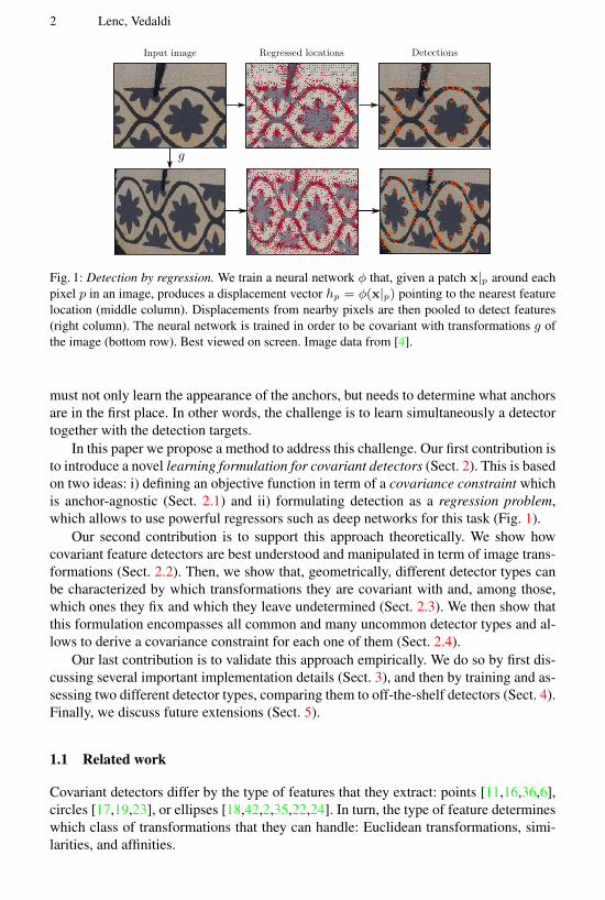
Fig. 1: Detection by regression. We train a neural network φ that, given a patch x|p around eachpixel p in an image, produces a displacement vector hp = φ(x|p) pointing to the nearest featurelocation (middle column). Displacements from nearby pixels are then pooled to detect features(right column). The neural network is trained in order to be covariant with transformations g ofthe image (bottom row). Best viewed on screen. Image data from [4].

must not only learn the appearance of the anchors, but needs to determine what anchorsare in the first place. In other words, the challenge is to learn simultaneously a detectortogether with the detection targets.

In this paper we propose a method to address this challenge. Our first contribution isto introduce a novel learning formulation for covariant detectors (Sect. 2). This is basedon two ideas: i) defining an objective function in term of a covariance constraint whichis anchor-agnostic (Sect. 2.1) and ii) formulating detection as a regression problem,which allows to use powerful regressors such as deep networks for this task (Fig. 1).

Our second contribution is to support this approach theoretically. We show howcovariant feature detectors are best understood and manipulated in term of image trans-formations (Sect. 2.2). Then, we show that, geometrically, different detector types canbe characterized by which transformations they are covariant with and, among those,which ones they fix and which they leave undetermined (Sect. 2.3). We then show thatthis formulation encompasses all common and many uncommon detector types and al-lows to derive a covariance constraint for each one of them (Sect. 2.4).

Our last contribution is to validate this approach empirically. We do so by first dis-cussing several important implementation details (Sect. 3), and then by training and as-sessing two different detector types, comparing them to off-the-shelf detectors (Sect. 4).Finally, we discuss future extensions (Sect. 5).

1.1 Related work

Covariant detectors differ by the type of features that they extract: points [11,16,36,6],circles [17,19,23], or ellipses [18,42,2,35,22,24]. In turn, the type of feature determineswhich class of transformations that they can handle: Euclidean transformations, simi-larities, and affinities.

Learning Covariant Feature Detectors 3

Another differentiating factor is the type of visual structures used as anchors.For instance, early approaches used corners extracted from an analysis of image ed-glets [29,8,34]. These were soon surpassed by methods that extracted corners and otheranchors using operators of the image intensity such as the Hessian of Gaussian [3] orthe structure tensor [7,11,47] and its generalizations [40]. In order to handle transfor-mations more complex than translations and rotations, scale selection methods using theLaplacian/Difference of Gaussian operator (L/DoG) were introduced [19,23], and fur-ther extended with affine adaptation [2,24] to handle full affine transformations. Whilethese are probably the best known detectors, several other approaches were explored aswell, including parametric feature models [9,28] and using self-dissimilarity [38,13].

All detectors discussed so far are handcrafted. Learning has been mostly limited tothe case in which detection anchors are defined a-priori, either by manual labelling [14]or as the output of a pre-existing handcrafted detetctor [5,31,39,12], with the goal ofaccelerating detection. Closer to our aim, [32] use simulated annealing to optimise theparameters of their FAST detector for repeatability. To the best of our knowledge, theonly line of work that attempted to learn repeatable anchors from scratch is the oneof [41,25], who did so using genetic programming; however, their approach is muchmore limited than ours, focusing only on the repeatability of corner points.

More recently, [44] learns to estimate the orientation of feature points using deeplearning. Contrary to our approach, the loss function is defined on top of the local imagefeature descriptors and is limited to estimating the rotation of keypoints. The workof [45,27,37] also use Siamese deep learning architectures for local features, but forlocal image feature description, whereas we use them for feature detection.

2 Method

We first introduce our method in a special case, namely in learning a basic corner de-tector (Sect. 2.1), and then we extend it to general covariant features (Sect. 2.2 and 2.3).Finally, we show how the theory applies to concrete examples of detectors (Sect. 2.4).

2.1 The covariance constraint

Let x be an image and let Tx be its version translated by T ∈ R2 pixels. A cornerdetector extracts from x a (small) collection of points f ∈ R2. The detector is said tobe covariant if, when applied to the translated image Tx, it returns the translated pointsf + T . Most covariant detectors work by anchoring features to image structures that,such as corners, are preserved under transformation. A challenge in defining anchorsis that these must be general enough to be found in most images and at the same timesufficiently distinctive to achieve covariance.

Anchor extraction is usually formulated as a selection problem by finding the fea-tures that maximize a handcrafted figure of merit such as Harris’ cornerness, the Lapla-cian of Gaussian, or the Hessian of Gaussian. This indirect construction makes learninganchors difficult. As a solution, we propose to regard feature detection not as a selectionproblem but as a regression one. Thus the goal is to learn a function ψ : x 7→ f that

4 Lenc, Vedaldi

Fig. 2: Left: an oriented circular frame f = gf0 is obtained as a unique similarity transformationg ∈ G of the canonical frame f0, where the orientation is represented by the dot. Concretely,this could be the output of the SIFT detector after orientation assignment. Middle: the detectorfinds feature frames fi = gif0, gi = φ(xi) in images x1 and x2 respectively due to covariance,matching the features allows to recover the underlying image transformation x2 = gx1 as g =g2 ◦ g−1

1 . Right: equivalently, then inverse transformations g−1i normalize the images, resulting

in the same canonical view.

directly maps an image (patch1) x to a corner f . The key advantage is that this functioncan be implemented by any regression method, including a deep neural network.

This leaves the problem of defining a learning objective. This would be easy if wehad example anchors annotated in the data; however, our aim is to discover useful an-chors automatically. Thus, we propose to use covariance itself as a learning objective.This is formally captured by the covariance constraint ψ(Tx) = T + ψ(x). A corre-sponding learning objective can be formulated as follows:

minψ

1

n

n∑i=1

‖ψ(Tixi)− ψ(xi)− Ti‖2 (1)

where (xi, Ti) are example patches and transformations and the optimization is overthe parameters of the regressor ψ (e.g. the filter weights in a deep neural network).

2.2 Beyond corners

This section provides a first generalization of the construction above. While simple de-tectors such as Harris extract 2D points f in correspondence of corners, others suchas SIFT extract circles in correspondence of blobs, and others again extract even morecomplex features such as oriented circles (e.g. SIFT with orientation assignment), el-lipses (e.g. Harris-Affine), oriented ellipses (e.g. Harris-Affine with orientation assign-ment), etc. In general, due to their role in fixing image transformations, we will call theextracted shapes f ∈ F feature frames.

The detector is thus a function ψ : X → F , x 7→ f mapping an image patch x toa corresponding feature frame f . We say that the detector is covariant with a group of

1 As the function ψ needs to be location invariant it can be applied in a sliding window manner.Therefore x can be a single patch which represents its perception field.

Learning Covariant Feature Detectors 5

transformations2 g ∈ G (e.g. similarity or affine) when

∀x ∈ X , g ∈ G : ψ(gx) = gψ(x) (2)

where gf is the transformed frame and gx is the warped image.3

Working with feature frames is intuitive, but cumbersome and not very flexible. Amuch better approach is to drop frames altogether and replace them with correspondingtransformations. For instance, in SIFT with orientation assignment all possible orientedcircles f can be expressed uniquely as a similarity gf0 of a fixed oriented circle f0(Fig. 2.left). Hence, instead of talking about oriented circles f , we can equivalently talkabout similarities g. Likewise, in the case of the Harris’ corner detector, all possible 2Dpoints f can be expressed as translations T + f0 of the origin f0, and so we can talkabout translations T instead of points f .

To generalize this idea, we say that that a class of frames F resolves a group oftransformations G when, given a fixed canonical frame f0 ∈ F , all frames are uniquelygenerated from it by the action of G:

F = Gf0 = {gf0 : g ∈ G} and ∀g, h ∈ G : gf0 = hf0 ⇒ g = h (uniqueness).

This bijective correspondence allows to “rename” frames with transformations. Usingthis renaming, the detector ψ can be rewritten as a function φ that outputs directly atransformation ψ(x) = φ(x)f0 instead of a frame.

With this substitution, the covariance constraint (2) becomes

φ(gx) ◦ φ(x)−1 ◦ g−1 = 1 . (3)

Note that, for the group of translationsG = T (2), this constraint corresponds directly tothe objective function (1). Fig. 2 provides two intuitive visualizations of this constraint.

It is also useful to extend the learning objective (1) as follows. As training data, weconsider n triplets (xi, xi, gi), i = 1, . . . , n comprising an image (patch) xi, a transfor-mation gi, and the transformed and distorted image xi = gxi + η. Here η representsadditive noise or some other useful distortion such as a random rescaling of the intensitywhich allows to train a more robust detector. The learning problem is then given by:

minφ

1

n

n∑i=1

d(ri, 1)2, ri = φ(xi) ◦ φ(xi)−1 ◦ g−1i (4)

where d(ri, 1)2 is the “distance” of the residual transformation ri from the identity.

2.3 General covariant feature extraction

The theory presented so far is insufficient to fully account for the properties of manycommon detectors. For this, we need to remove the assumptions that feature frames

2 Here, a group of transformation (G, ◦) is a set of functions g, h : R2 → R2 together withcomposition g◦h ∈ G as group operation. Composition is associative; furthermore,G containsthe identity transformation 1 and the inverse g−1 of each of its elements g ∈ G.

3 The action gx of the transformation g on the image x is to warp it: (gx)(u, v) = x(g−1(u, v))

6 Lenc, Vedaldi

Fig. 3: Left: a (unoriented) circle identifies the translation and scale component of a similaritytransformation g ∈ G, but leaves a residual rotation q ∈ Q undetermined. Concretely, this couldbe the output of the SIFT detector prior orientation assignment. Right: normalization is achievedup to the residual transformation q.

resolve (i.e. fix) completely the group of transformations G. Most detectors are in factcovariant with transformation groups larger than the ones that they can resolve. Forexample, the Harris’s detector is covariant with rotation and translation (in the sensethat the same corners are extracted after the image is roto-translated), but, by detecting2D points, it only resolves translations. Likewise, SIFT without orientation assignmentis covariant to full similarity transformations but, by detecting circles, only resolvesdilations (i.e. rotations remains undetermined; Fig. 3).

Next, we explain how eq. (3) must be modified to deal with detectors that (i) arecovariant with a transformation group G but (ii) resolve only a subgroup H ⊂ G. Inthis case, the detector function φ(x) ∈ H returns a transformation in the smaller groupH , and the covariance constraint (3) is satisfied up to a complementary transformationq ∈ Q that makes up for the part not resolved by the detector:

∃q ∈ Q : φ(gx) ◦ q ◦ φ(x)−1 ◦ g−1 = 1. (5)

This situation is illustrated graphically in Fig. 3.For this construction to work, given H ⊂ G, the group Q ⊂ G must be chosen

appropriately. In eq. (5), and following Fig. 3, call h1 = φ(x) and h2 = φ(gx). Rear-ranging the terms, we get that h2q = h1g, where h2 ∈ H, q ∈ Q and h1g ∈ G. Thismeans that any element in G must be expressible as a composition hq, i.e. G = HQ ={hq : h ∈ H, q ∈ Q}. Formally (proofs in appendix):

Proposition 1. If the group G = HQ is the product of the subgroups H and Q, then,for any choice of g ∈ G and h1 ∈ H , there is always a decomposition

h2qh−11 g−1 = 1, such that h2 ∈ H, q ∈ Q. (6)

In practice, given G and H , Q is usually easily found as the “missing transforma-tion”; however, compared to (2), the transformation q in constraint (5) is an extra de-gree of freedom that complicates optimization. Fortunately, in many cases the followingproposition shows that there is only one possible q:

Proposition 2. If H / G is normal in G (i.e. ∀g ∈ G, h ∈ H : g−1hg ∈ H) andH ∩Q = {1}, then, given g ∈ G, the choice of q in the decomposition (5) is unique.

The next section works through several concrete examples to illustrate these con-cepts.

Learning Covariant Feature Detectors 7

2.4 A taxonomy of detectors

This section applies the theory developed above to standard detectors. Concretely, welimit ourselves to transformations up to affine, and write:

hi =

[Mi Pi0 1

], q =

[L 00 1

], g =

[A T0 1

].

Here Pi can be interpreted as the centre of the feature in image xi and Mi as its affineshape, (A, T ) as the parameters of the image transformation, and L as the parameterof the complementary transformation not fixed by the detector. The covariance con-straint (5) can be written, after a short calculation, as

M2LM−11 = A, P2 −AP1 = T. (7)

As a first example, consider a basic corner detector that resolves translations H =G = T (2) with no (non-trivial) complementary transformation Q = {1}. Hence M1 =M2 = L = A = I and (5) becomes:

P2 − P1 = T. (8)

This is the same expression found in the simple example of Sect. 2.1 and requires thedetected features to have the correct relative shift T .

The Harris corner detector is similar, but is covariant with rotations too. Formally,H = T (2) ⊂ G = SE(2) (Euclidean transforms) and Q = SO(2) (rotations). SinceT (2) / SE(2) is a normal subgroup, we expect to find a unique choice for q. In fact, itmust be Mi = I , A = L = R, and the constraint reduces to:

P2 −RP1 = T. (9)

In SIFT, G = S(2) is the group of similarities, so that A = sR is the compositionof a rotation R ∈ SO(2) and an isotropic scaling s ∈ R+. SIFT prior to orientationassignment resolves the subgroupH of dilations (scaling and translation), so thatMi =σiI (scaling) and the complement is a rotation L ∈ SO(2). Once again H / G, so thechoice of q is unique, and in particular L = R. The constraint reduces to:

P2 − sRP1 = T, σ2/σ1 = s. (10)

When orientation assignment is added to SIFT, the similarities are completely resolvedH = G = S(2), Mi = σiRi is a rotation and scaling, and the constraint becomes:

P2 − sRP1 = T, σ2/σ1 = s, R2R>1 = R. (11)

Affine detectors such as Harris-Affine (without orientation assignment) are morecomplex. In this case G = A(2) are affinities and H = UA(2) are upright affinities, i.e.affinities where the linear map Mi ∈ LT+(2) is a lower-triangular matrix with positivediagonal (these affinities, which still form a group, leave the “up” direction unchanged).The residual Q = SO(2) are rotations and HQ = G is still satisfied. However, UA(2)

8 Lenc, Vedaldi

is not normal in A(2), Prop. 2 does not apply, and the choice of Q is not unique.4 Theconstraint has the form:

P2 −AP1 = T, M−12 AM1 ∈ SO(2). (12)

For affine detectors with orientation assignment, H = G = A(2) and the constraint is:

P2 −AP1 = T, M2M−11 = A. (13)

The generality of our formulation allows learning many new types of detectors. Forexample, by setting H = T (2) and G = A(2) it is possible to train a corner detectorsuch as Harris which is covariant to full affine transformations. Furthermore, a benefitof working with transformations instead of feature frames is that we can train detectorsthat would be difficult to express in terms of geometric primitives. For instance, bysetting H = SO(2) and G = SE(2), we can train a orientation detector which iscovariant with rotation and translation. As for affine upright features, in this case His not normal in G so the complementary translation q = (I, T ′) ∈ Q is not uniquelyfixed by g = (R, T ) ∈ G; nevertheless, a short calculation shows that the only partof (5) that matters in this case is

R>2 R1 = R (14)

where hi = (Ri, 0) are the rotations estimated by the regressor.

3 Implementation

This section discusses several implementation details of our method: the parametriza-tion of transformations, example CNN architectures, multiple features detection, effi-cient dense detection, and preparing the training data.

Transformations: parametrization and loss. Implementing (4) requires parametrizingthe transformation φ(x) ∈ H predicted by the regressor. In the most general case ofinterest here, H = A(2) are affine transformations and the simplest approach is tooutput the corresponding matrix of coefficients:

φ(x) =

[a b p0 0 1

]=

au bu puav bv pv0 0 1

.Here p can be interpreted as the feature center and a and b as the feature affine shape.By rearranging the terms in (2), the loss function in (4) takes the form

d2(r, 1) = minq∈Q‖gφ(x)− φ(gx)q‖2F , (15)

where ‖ · ‖F is the Frobenius norm. As seen before, the complementary transformationq is often uniquely determined given g and the minimization can be removed by sub-stituting this fixed value for q. In practice, g and q are also represented by matrices, asdescribed in Sect. 2.4.

4 Concretely, from M2L = AM1 the complement matrix L is given by the QR decompositionof the r.h.s. which is a function of M1, i.e. not unique.

Learning Covariant Feature Detectors 9

Table 1: Network architectures. The DetNet-S and DetNet-L CNN architectures used which con-sist of a small number of convolutional layers applied densely and with no padding. The filtersizes and number is specified in the top part of each cell. Filters are followed by ReLU layersand, where indicated, by 2× 2 max pooling and/or LRN.

Model Conv1 Conv2 Conv3 Conv4 Conv5 Conv6 Conv7

DetNet-S 5× 5× 40 5× 5× 100 4× 4× 300 1× 1× 500 1× 1× 500 1× 1× 2Pool ↓ 2 Pool ↓ 2

DetNet-L 5× 5× 60 5× 5× 150 4× 4× 450 1× 1× 600 1× 1× 600 1× 1× 600 1× 1× 2Pool ↓ 2 Pool ↓ 2 + LRN

When the resolved transformationsH are less general than affinities, the parametriza-tion can be adjusted accordingly. For instance, for the basic detector of Sect. 2.1, whereH = T (2), on can fix a = (1, 0), b = (0, 1), q = I and g = (I, T ), which reduces toeq. (1). If, on the other hand, H = SO(2) are rotation matrices as for the orientationdetector (14),

φ(x) =1√

a2u + a2v

au −av 0av au 00 0 1

. (16)

Network architectures. One of the benefits of our approach is that it allows to use deepneural networks in order to implement the feature regressor φ(x). Here we experimentwith two such architectures, DetNet-S and DetNet-L, summarized in Tab. 1. For fast de-tection, these resemble the compact LeNet model of [15]. The main difference betweenthe two is the number of layers and filters. The loss (15) is differentiable and easilyimplemented in a network loss layer. Note that the loss requires evaluating the networkφ twice, once applied to image x and once to image gx. Like in siamese architectures,these can be thought of as two networks with shared weights.

When implemented in a standard CNN toolbox (in our case in MatConvNet [43]),multiple patch pairs are processed in parallel by a single CNN execution in what isknown as a minibatch. In practice, the operations in (15) can be implemented usingoff-the-shelf CNN components. For example, the multiplication by the affine transfor-mation g in (15), which depends on which pair of images in the batch is considered,can be implemented by using convolution routines, 1 × 1 filters, and so called “filtergroups”.

From local regression to global detection. The formulation (4) learns a function ψ thatmaps an image patch x to a single detected feature f = ψ(x). In order to detect multiplefeatures in a larger image, the function ψ is simply applied convolutionally at all imagelocations (Fig. 1). Then, due to covariance, partially overlapping patches x that containthe same feature are mapped by ψ to the same detection f . Such duplicate detectionsare collapsed and their number, which reflects the stability of the feature, is used asdetection confidence.

For point features (G = T (2)), this voting process is implemented efficiently byaccumulating votes in a map containing one bin for each pixel in the input image. Votesare accumulated using bilinear interpolation, after which non-maxima suppression isapplied with a radius of two pixels. This scheme can be easily extended to more complex

10 Lenc, Vedaldi

DETNET

Trai

nE

asy

Har

d

DETNET

Trai

nE

asy

Har

d

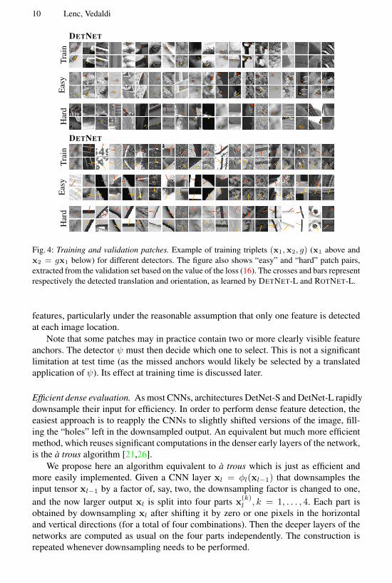
Fig. 4: Training and validation patches. Example of training triplets (x1,x2, g) (x1 above andx2 = gx1 below) for different detectors. The figure also shows “easy” and “hard” patch pairs,extracted from the validation set based on the value of the loss (16). The crosses and bars representrespectively the detected translation and orientation, as learned by DETNET-L and ROTNET-L.

features, particularly under the reasonable assumption that only one feature is detectedat each image location.

Note that some patches may in practice contain two or more clearly visible featureanchors. The detector ψ must then decide which one to select. This is not a significantlimitation at test time (as the missed anchors would likely be selected by a translatedapplication of ψ). Its effect at training time is discussed later.

Efficient dense evaluation. As most CNNs, architectures DetNet-S and DetNet-L rapidlydownsample their input for efficiency. In order to perform dense feature detection, theeasiest approach is to reapply the CNNs to slightly shifted versions of the image, fill-ing the “holes” left in the downsampled output. An equivalent but much more efficientmethod, which reuses significant computations in the denser early layers of the network,is the a trous algorithm [21,26].

We propose here an algorithm equivalent to a trous which is just as efficient andmore easily implemented. Given a CNN layer xl = φl(xl−1) that downsamples theinput tensor xl−1 by a factor of, say, two, the downsampling factor is changed to one,and the now larger output xl is split into four parts x

(k)l , k = 1, . . . , 4. Each part is

obtained by downsampling xl after shifting it by zero or one pixels in the horizontaland vertical directions (for a total of four combinations). Then the deeper layers of thenetworks are computed as usual on the four parts independently. The construction isrepeated whenever downsampling needs to be performed.

Learning Covariant Feature Detectors 11

Detection speed can be improved with evaluating the regressor with stride 2 (atevery second pixel). We refer to these detector as DETNETS2. Source code and theDETNETmodels are freely available5.

Training data. Training images are obtained from the ImageNet ILSVRC 2012 trainingdata [33], extracting twenty random 57 × 57 crops per image, for up to 6M crops.Uniform crops are discarded since they clearly cannot contain any useful anchor. Todo so, the absolute response of a LoG filter of variance σ = 2.5 is averaged and thecrop is retained if the response is greater than 1.5 (image intensities are in the range[0, 255]). Note that, combined with random selection, this operation does not centercrops on blobs or any other pre-defined anchors, but simply discards uniform or verylow contrast crops.

Recall that the formulation Sect. 2.2 requires triplets (x1,x2, g). A triplet is gen-erated by randomly picking a crop and then by extracting 28 × 28 patches x1 and x2

within 20 pixels of the crop center (Fig. 4). This samples two patches related by trans-lation, corresponding to the translation sampled in g, while guaranteeing that patchesoverlap by least 27%. Then the linear part of g is sampled at random and used to warp x2

around its center. In order too achieve better robustness to photometric transformations,additive (±8% of the intensity range) and multiplicative (±40% of a pixel intensity) isadded to the pixels .

Training uses batches of 64 patch pairs. An epoch contains 40 · 103 pairs, and thedata is resampled after each epoch completes. The learning rate is set to λ = 0.01and decreased tenfold when the validation error stops decreasing. Usually, training con-verges after 60 epochs, which, due to the small size of the network and input patches,takes no more than a couple of minutes on a GPU.

4 Experiments

We apply our framework to learn two complementary types of detectors in order toillustrate the flexibility of the approach: a corner detector (Sect. 4.1) and an orientationdetector (Sect. 4.2).

Evaluation benchmark and metrics. We compare the learned detectors to standard ones:FAST [31,30] (using OpenCV’s implementation6), the Difference of Gaussian detector(DoG) or SIFT [20], the Harris corner point detector [11] and Hessian point detector[24] (all using VLFeat’s implementation7). All experiments are performed at a singlescale, but all detectors can be applied to a scale space pyramid if needed.

For evaluation of the corner detector, we use the standard VGG-Affine benchmarkdataset [24], using both the repeatability and matching score criteria. For matchingscore, SIFT descriptors are extracted from a fixed region of 41× 41 pixels around eachcorner. A second limitation in the original protocol of [24] is that repeatability can bemade arbitrarily large simply by detecting enough features. Thus, in order to control

5 https://github.com/lenck/ddet6 opencv.org7 www.vlfeat.org

12 Lenc, Vedaldi

-40.0 -30.0 -20.0 -10.0 1.7 11.7 21.7 31.70.4

0.7

1

Arc 1, viewpoint angle

Rep

atab

ility

-25.0 -18.1 -11.2 -4.3 2.6 9.5 16.4 23.30.15

0.2

0.25

Arc 2, viewpoint angle-20.0 -13.3 -6.7 0.0 6.7 13.3 20.0

0.1

0.15

0.2

Arc 3, viewpoint angle

DetNet-L DetNet-S DoG Harris Hessian FAST

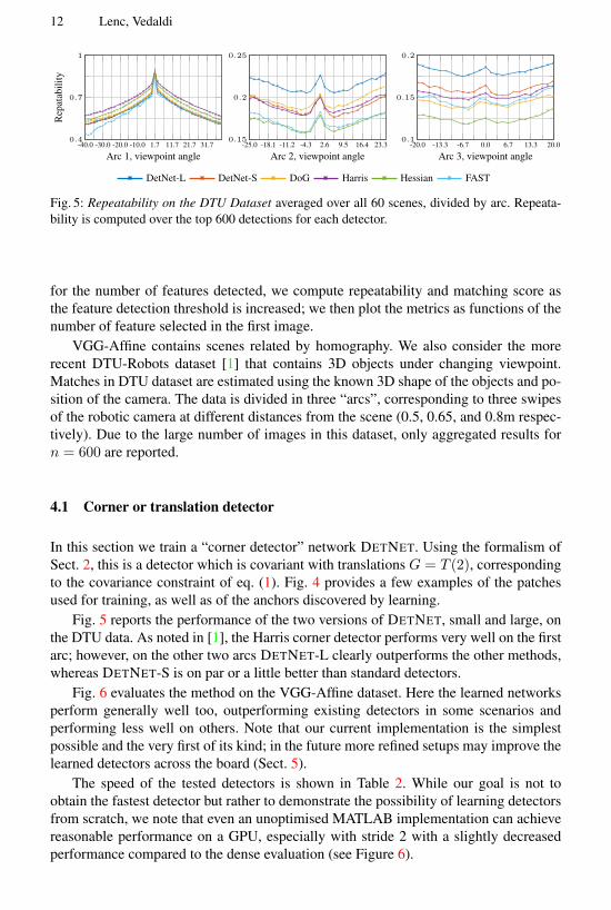
Fig. 5: Repeatability on the DTU Dataset averaged over all 60 scenes, divided by arc. Repeata-bility is computed over the top 600 detections for each detector.

for the number of features detected, we compute repeatability and matching score asthe feature detection threshold is increased; we then plot the metrics as functions of thenumber of feature selected in the first image.

VGG-Affine contains scenes related by homography. We also consider the morerecent DTU-Robots dataset [1] that contains 3D objects under changing viewpoint.Matches in DTU dataset are estimated using the known 3D shape of the objects and po-sition of the camera. The data is divided in three “arcs”, corresponding to three swipesof the robotic camera at different distances from the scene (0.5, 0.65, and 0.8m respec-tively). Due to the large number of images in this dataset, only aggregated results forn = 600 are reported.

4.1 Corner or translation detector

In this section we train a “corner detector” network DETNET. Using the formalism ofSect. 2, this is a detector which is covariant with translations G = T (2), correspondingto the covariance constraint of eq. (1). Fig. 4 provides a few examples of the patchesused for training, as well as of the anchors discovered by learning.

Fig. 5 reports the performance of the two versions of DETNET, small and large, onthe DTU data. As noted in [1], the Harris corner detector performs very well on the firstarc; however, on the other two arcs DETNET-L clearly outperforms the other methods,whereas DETNET-S is on par or a little better than standard detectors.

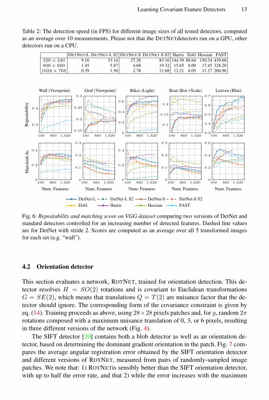
Fig. 6 evaluates the method on the VGG-Affine dataset. Here the learned networksperform generally well too, outperforming existing detectors in some scenarios andperforming less well on others. Note that our current implementation is the simplestpossible and the very first of its kind; in the future more refined setups may improve thelearned detectors across the board (Sect. 5).

The speed of the tested detectors is shown in Table 2. While our goal is not toobtain the fastest detector but rather to demonstrate the possibility of learning detectorsfrom scratch, we note that even an unoptimised MATLAB implementation can achievereasonable performance on a GPU, especially with stride 2 with a slightly decreasedperformance compared to the dense evaluation (see Figure 6).

Learning Covariant Feature Detectors 13

Table 2: The detection speed (in FPS) for different image sizes of all tested detectors, computedas an average over 10 measurements. Please not that the DETNETdetectors run on a GPU, otherdetectors run on a CPU.

DETNET-L DETNET-L S2 DETNET-S DETNET-S S2 Harris DoG Hessian FAST320× 240 9.16 33.14 27.26 83.16 144.39 88.64 150.34 439.68800× 600 1.45 5.87 4.68 19.32 15.65 8.00 17.45 328.201024× 768 0.39 1.56 2.78 11.68 12.21 6.05 11.17 206.96

Wall (Viewpoint) Graf (Viewpoint) Bikes (Light) Boat (Rot.+Scale) Leuven (Blur)

100 860 1,620

0.2

0.4

Rep

eata

bilit

y

100 860 1,620

0.15

0.2

0.25

0.3

100 860 1,6200

0.2

0.4

0.6

100 860 1,620

0.1

0.15

0.2

100 860 1,6200.3

0.4

0.5

0.6

0.7

100 860 1,6200

0.2

0.4

Num. Features

Mat

chin

hSc

.

100 860 1,6200

0.1

0.2

0.3

Num. Features100 860 1,620

0

0.2

0.4

Num. Features100 860 1,620

0

0.1

0.2

0.3

Num. Features100 860 1,620

0

0.2

0.4

0.6

Num. Features

DetNet-L DetNet-L S2 DetNet-S DetNet-S S2DoG Harris Hessian FAST

Fig. 6: Repeatability and matching score on VGG dataset comparing two versions of DetNet andstandard detectors controlled for an increasing number of detected features. Dashed line valuesare for DetNet with stride 2. Scores are computed as an average over all 5 transformed imagesfor each set (e.g. “wall”).

4.2 Orientation detector

This section evaluates a network, ROTNET, trained for orientation detection. This de-tector resolves H = SO(2) rotations and is covariant to Euclidean transformationsG = SE(2), which means that translations Q = T (2) are nuisance factor that the de-tector should ignore. The corresponding form of the covariance constraint is given byeq. (14). Training proceeds as above, using 28×28 pixels patches and, for g, random 2πrotations composed with a maximum nuisance translation of 0, 3, or 6 pixels, resultingin three different versions of the network (Fig. 4).

The SIFT detector [20] contains both a blob detector as well as an orientation de-tector, based on determining the dominant gradient orientation in the patch. Fig. 7 com-pares the average angular registration error obtained by the SIFT orientation detectorand different versions of ROTNET, measured from pairs of randomly-sampled imagepatches. We note that: 1) ROTNETis sensibly better than the SIFT orientation detector,with up to half the error rate, and that 2) while the error increases with the maximum

14 Lenc, Vedaldi

0 2 40

25

50

75

100

Max Displacement [px]

Avg

.Ang

leer

ror[

deg]

SIFTRNRN+TR3RN+TR6

Matching score (%)graf boat bark bikes leuven

SIFT 68.0 73.7 75.3 81.8 85.2ROTNET-L 67.3 74.3 81.1 83.0 85.2

Fig. 7: Orientation detector evaluation. Left: versions of ROTNET(RN) and the SIFT orientationdetector evaluated on recovering the relative rotation of random patch pairs. Right: matchingscore on the VGG-Affine benchmark when the native SIFT orientation estimation is replacedwith ROTNET(percentage of correct matches using the DoG-Affine detector).

nuisance translation between patches, networks that are trained to account for suchtranslations are sensibly better than the ones that do not. Furthermore, when applied tothe output of the SIFT blob detector, the improved orientation estimation results in animproved feature matching score, as measured on the VGG-Affine benchmark.

5 Discussion

We have presented the first general machine learning formulation for covariant featuredetectors. The latter is supported by a comprehensive theory of covariant detectors, andbuilds on the idea of casting detection as a regression problem. We have shown that thismethod can successfully learn corner and orientation detectors that outperform in sev-eral cases off-the-shelf detectors. The potential is significant; for example, the frame-work can be used to learn scale selection and affine adaptation CNNs. Furthermore,many significant improvements to our basic implementation are possible, including ex-plicitly modelling detection strength/confidence, predicting multiple features in a patch,and jointly training detectors and descriptors.

Acknowledgements We would like to thank ERC 677195-IDIU for supporting thisresearch.

A Proofs

Proof (of Proposition 1). Due to group closure, gh1 ∈ G. Since HQ = G, then theremust be h2 ∈ H, q ∈ Q such that h2q = gh1, and so h2qh−11 g−1 = 1.

Proof (of Proposition 2). Let h2q(h1)−1 = h′2q′(h′1)

−1 be two such decompositionsand multiply to the left by (q)−1(h′2)

−1 and to the right by h′1:

q−1 [(h′2)−1h2] q︸ ︷︷ ︸

∈H (due to normality)

h−11 h′1︸ ︷︷ ︸∈H

= q−1q′︸ ︷︷ ︸∈Q

.

Since this quantity is simultaneously inH and inQ, it must be in the intersectionH∩Q,which by hypothesis contains only the identity. Hence q−1q′ = 1 and q = q′.

Learning Covariant Feature Detectors 15

References

1. H. Aanæs, A. Dahl, and K. Steenstrup Pedersen. Interesting interest points. InternationalJournal of Computer Vision, pages 18–35, 2012. 12

2. A. M. Baumberg. Reliable feature matching across widely separated views. In Proc. CVPR,pages 774–781, 2000. 2, 3

3. P. R. Beaudet. Rotationally invariant image operators. In International Joint Conference onPattern Recognition, volume 579, page 583, 1978. 3

4. K. Cordes, B. Rosenhahn, and J. Ostermann. Increasing the accuracy of feature evalua-tion benchmarks using differential evolution. In IEEE Symposium on Differential Evolution,2011. 2

5. P. Dias, A. Kassim, and V. Srinivasan. A neural network based corner detection method. InIEEE Int. Conf. on Neural Networks, 1995. 3

6. Y. Dufournaud, C. Schmid, and R. Horaud. Matching images with different resolutions. InProc. CVPR, 1999. 2

7. W. Forstner. A feature based correspondence algorithm for image matching. InternationalArchives of Photogrammetry and Remote Sensing, 26(3):150–166, 1986. 3

8. H. Freeman and L. S. Davis. A corner-finding algorithm for chain-coded curves. IEEETransactions on Computers, (3):297–303, 1977. 3

9. A. Guiducci. Corner characterization by differential geometry techniques. Pattern Recogni-tion Letters, 8(5):311–318, 1988. 3

10. X. Han, T. Leung, Y. Jia, R. Sukthankar, and A. C. Berg. Matchnet: Unifying feature andmetric learning for patch-based matching. In Proc. CVPR, 2015. 1

11. C. Harris and M. Stephens. A combined corner and edge detector. In Proc. of The FourthAlvey Vision Conference, pages 147–151, 1988. 2, 3, 11

12. S. Holzer, J. Shotton, and P. Kohli. Learning to efficiently detect repeatable interest points indepth data. In Proc. ECCV, 2012. 3

13. T. Kadir and M. Brady. Saliency, scale and image description. Int. J. Computer Vision,45:83–105, 2001. 3

14. W. Kienzle, F. A. Wichmann, B. Scholkopf, and M. O. Franz. Learning an interest operatorfrom human eye movements. In CVPR Workshop, 2006. 3

15. Y. Lecun, L. Bottou, Y. Bengio, and P. Haffner. Gradient-based learning applied to documentrecognition. Proceedings of the IEEE, Nov 1998. 9

16. T. Lindeberg. Scale-Space Theory in Computer Vision. Springer, 1994. 217. T. Lindeberg. Feature detection with automatic scale selection. IJCV, 30(2):77–116, 1998.

218. T. Lindeberg and J. Garding. Shape-adapted smoothing in estimation of 3-D depth cues from

affine distortions of local 2-D brightness structure. In Proc. ECCV, 1994. 219. D. G. Lowe. Object recognition from local scale-invariant features. In Proc. ICCV, 1999. 2,

320. D. G. Lowe. Distinctive image features from scale-invariant keypoints. IJCV, 2(60):91–110,

2004. 11, 1321. S. Mallat. A Wavelet Tour of Signal Processing. Academic Press, 2008. 1022. J. Matas, S. Obdrzalek, and O. Chum. Local affine frames for wide-baseline stereo. In Intl.

Conference on Pattern Recognition, 2002. 223. K. Mikolajczyk and C. Schmid. Indexing based on scale invariant interest points. In Proc.

ICCV, 2001. 2, 324. K. Mikolajczyk and C. Schmid. An affine invariant interest point detector. In Proc. ECCV,

pages 128–142. Springer-Verlag, 2002. 2, 3, 1125. G. Olague and L. Trujillo. Evolutionary-computer-assisted design of image operators that

detect interest points using genetic programming. Image and Vision Computing, 2011. 3

16 Lenc, Vedaldi

26. G. Papandreou, I. Kokkinos, and P.-A. Savalle. Modeling local and global deformations indeep learning: Epitomic convolution, multiple instance learning, and sliding window detec-tion. Proc. CVPR, 2015. 10

27. M. Paulin, M. Douze, Z. Harchaoui, J. Mairal, F. Perronin, and C. Schmid. Local convolu-tional features with unsupervised training for image retrieval. In ICCV, 2015. 3

28. K. Rohr. Recognizing corners by fitting parametric models. IJCV, 9(3), 1992. 329. A. Rosenfeld and E. Johnston. Angle detection on digital curves. Computers, IEEE Trans-

actions on, 100(9):875–878, 1973. 330. E. Rosten and T. Drummond. Fusing points and lines for high performance tracking. In

ICCV, volume 2, 2005. 1131. E. Rosten and T. Drummond. Machine learning for high-speed corner detection. In Proc.

ECCV, 2006. 3, 1132. E. Rosten, R. Porter, and T. Drummond. Faster and better: a machine learning approach to

corner detection. In PAMI, volume 32, 2010. 333. O. Russakovsky, J. Deng, H. Su, J. Krause, S. Satheesh, S. Ma, Z. Huang, A. Karpathy,

A. Khosla, M. Bernstein, A. C. Berg, and L. Fei-Fei. Imagenet large scale visual recognitionchallenge, 2014. 11

34. P. Sankar and C. Sharma. A parallel procedure for the detection of dominant points on adigital curve. Computer Graphics and Image Processing, 7(3):403–412, 1978. 3

35. F. Schaffalitzky and A. Zisserman. Viewpoint invariant texture matching and wide baselinestereo. In Proc. ICCV, 2001. 2

36. C. Schmid and R. Mohr. Local greyvalue invariants for image retrieval. Pattern Analysis andMachine Intelligence, IEEE Transactions on, 1997. 2

37. E. Simo-Serra, E. Trulls, L. Ferraz, I. Kokkinos, P. Fua, and F. Moreno-Noguer. Discrimina-tive learning of deep convolutional feature point descriptors. In ICCV, 2015. 3

38. S. M. Smith and J. M. Brady. Susan – a new approach to low level image processing.Technical report, Oxford University, 1995. 3

39. J. Sochman and J. Matas. Learning fast emulators of binary decision processes. IJCV, 2009.3

40. B. Triggs. Detecting keypoints with stable position, orientation, and scale under illuminationchanges. In Proc. ECCV, 2004. 3

41. L. Trujillo and G. Olague. Synthesis of interest point detectors through genetic programming.In Proc. GECCO, 2006. 3

42. T. Tuytelaars and L. Van Gool. Wide baseline stereo matching based on local, affinely in-variant regions. In Proc. BMVC, pages 412–425, 2000. 2

43. A. Vedaldi and K. Lenc. Matconvnet – convolutional neural networks for matlab. In Proc.ACM Int. Conf. on Multimedia, 2015. 9

44. K. M. Yi, Y. Verdie, P. Fua, and V. Lepetit. Learning to Assign Orientations to Feature Points.In CVPR, 2016. 3

45. S. Zagoruyko and N. Komodakis. Learning to compare image patches via convolutionalneural networks. In CVPR, 2015. 3

46. J. Zbontar and Y. LeCun. Computing the stereo matching cost with a convolutional neuralnetwork. In Proc. CVPR, 2015. 1

47. M. Zuliani, C. Kenney, and B. S. Manjunath. A mathematical comparison of point detectors.In Proc. CVPR, 2005. 3