learning bayesian classifiers for scene classification

IEEE TRANSACTIONS ON GEOSCIENCE AND REMOTE SENSING, VOL. 43, NO. 3, MARCH 2005 581

Learning Bayesian Classifiers for SceneClassification With a Visual Grammar

Selim Aksoy, Member, IEEE, Krzysztof Koperski, Member, IEEE, Carsten Tusk, Giovanni Marchisio, Member, IEEE,and James C. Tilton, Senior Member, IEEE

Abstract—A challenging problem in image content extractionand classification is building a system that automatically learnshigh-level semantic interpretations of images. We describe aBayesian framework for a visual grammar that aims to reducethe gap between low-level features and high-level user semantics.Our approach includes modeling image pixels using automaticfusion of their spectral, textural, and other ancillary attributes;segmentation of image regions using an iterative split-and-mergealgorithm; and representing scenes by decomposing them intoprototype regions and modeling the interactions between these re-gions in terms of their spatial relationships. Naive Bayes classifiersare used in the learning of models for region segmentation andclassification using positive and negative examples for user-de-fined semantic land cover labels. The system also automaticallylearns representative region groups that can distinguish differentscenes and builds visual grammar models. Experiments usingLandsat scenes show that the visual grammar enables creation ofhigh-level classes that cannot be modeled by individual pixels orregions. Furthermore, learning of the classifiers requires only afew training examples.

Index Terms—Data fusion, image classification, image segmen-tation, spatial relationships, visual grammar.

I. INTRODUCTION

THE AMOUNT of image data that is received from satel-lites is constantly increasing. For example, the National

Aeronautics and Space Administration (NASA) Terra satel-lite sends more than 850 GB of data to the earth every day(http://terra.nasa.gov). Automatic content extraction, classifi-cation, and content-based retrieval have become highly desiredgoals for developing intelligent databases for effective andefficient processing of remotely sensed imagery. Most of theprevious approaches try to solve the content extraction problemby building pixel-based classification and retrieval modelsusing spectral and textural features. However, there is a largesemantic gap between low-level features and high-level userexpectations and scenarios. This semantic gap makes a humanexpert’s involvement and interpretation in the final analysis

Manuscript received March 15, 2004; revised September 28, 2004. Thiswork was supported by the National Aeronautics and Space Administrationunder Contracts NAS5-98053 and NAS5-01123. The VisiMine project wasalso supported by the U.S. Army under Contracts DACA42-03-C-16 andW9132V-04-C-0001.

S. Aksoy is with the Department of Computer Engineering, Bilkent Univer-sity, Ankara 06800, Turkey (e-mail: [email protected]).

K. Koperski, C. Tusk, and G. Marchisio are with Insightful Corporation,Seattle, WA 98109 USA (e-mail: [email protected]; [email protected];[email protected]).

J. C. Tilton is with NASA Goddard Space Flight Center, Greenbelt, MD20771 USA (e-mail: [email protected]).

Digital Object Identifier 10.1109/TGRS.2004.839547

inevitable, and this makes processing of data in large remotesensing archives practically impossible.

The commonly used statistical classifiers model image con-tent using distributions of pixels in spectral or other featuredomains by assuming that similar land cover structures willcluster together and behave similarly in these feature spaces.Schröder et al. [1] developed a system that uses Bayesian clas-sifiers to represent high-level land cover labels for pixels usingtheir low-level spectral and textural attributes. They used theseclassifiers to retrieve images from remote sensing archives byapproximating the probabilities of images belonging to differentclasses using pixel-level probabilities.

However, an important element of image understanding is thespatial information because complex land cover structures usu-ally contain many pixels and regions that have different featurecharacteristics. Furthermore, two scenes with similar regionscan have very different interpretations if the regions have dif-ferent spatial arrangements. Even when pixels and regions canbe identified correctly, manual interpretation is often necessaryfor many applications of remote sensing image analysis like landcover classification, urban mapping and monitoring, and ecolog-ical analysis in public health studies [2]. These applications willbenefit greatly if a system can automatically learn high-level se-mantic interpretations of scenes instead of classification of onlythe individual pixels.

The VisiMine system [3] we have developed supports inter-active classification and retrieval of remote sensing images byextending content modeling from pixel level to region and scenelevels. Pixel-level characterization provides classification de-tails for each pixel with automatic fusion of its spectral, textural,and other ancillary attributes. Following a segmentation process,region-level features describe properties shared by groups ofpixels. Scene-level features model the spatial relationships ofthe regions composing a scene using a visual grammar. This hi-erarchical scene modeling with a visual grammar aims to bridgethe gap between features and semantic interpretation.

This paper describes our work on learning the visual grammarfor scene classification. Our approach includes learning pro-totypes of primitive regions and their spatial relationships forhigher level content extraction. Bayesian classifiers that requireonly a few training examples are used in the learning process.Early work on syntactical description of images includes thepicture description language [4] that is based on operators thatrepresent the concatenations between elementary picture com-ponents like line segments in line drawings. More advancedimage processing and computer vision-based approaches onmodeling spatial relationships of regions include using cen-troid locations and minimum bounding rectangles to computeabsolute and relative locations [5]. Centroids and minimum

0196-2892/$20.00 © 2005 IEEE

582 IEEE TRANSACTIONS ON GEOSCIENCE AND REMOTE SENSING, VOL. 43, NO. 3, MARCH 2005

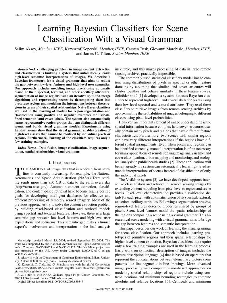
Fig. 1. Object/process diagram for the system. Rectangles represent objectsand ellipses represent processes.

bounding rectangles are useful when regions have circularor rectangular shapes, but regions in natural scenes often donot follow these assumptions. More complex representationsof spatial relationships include spatial association networks[6], knowledge-based spatial models [7], [8], and attributedrelational graphs [9]. However, these approaches require eithermanual delineation of regions by experts or partitioning ofimages into grids. Therefore, they are not generally applicabledue to the infeasibility of manual annotation in large databasesor because of the limited expressiveness of fixed sized grids.

Our work differs from other approaches in that recognitionof regions and decomposition of scenes are done automaticallyafter the system learns region and scene models with only asmall amount of supervision in terms of positive and negativeexamples for classes of interest. The rest of the paper is orga-nized as follows. An overview of the visual grammar is givenin Section II. The concept of prototype regions is defined inSection III. Spatial relationships of these prototype regions aredescribed in Section IV. Image classification using the visualgrammar models is discussed in Section V. Conclusions aregiven in Section VI.

II. VISUAL GRAMMAR

We are developing a visual grammar [10], [11] for interactiveclassification and retrieval in remote sensing image databases.This visual grammar uses hierarchical modeling of scenes inthree levels: pixel level, region level, and scene level. Pixel-levelrepresentations include labels for individual pixels computedin terms of spectral features, Gabor [12] and cooccurrence[13] texture features, elevation from digital elevation models(DEMs), and hierarchical segmentation cluster features [14].Region-level representations include land cover labels forgroups of pixels obtained through region segmentation. Theselabels are learned from statistical summaries of pixel contentsof regions using mean, standard deviation, and histograms,and from shape information like area, boundary roughness,orientation, and moments. Scene-level representations includeinteractions of different regions computed in terms of theirspatial relationships.

The object/process diagram of our approach is given in Fig. 1,where rectangles represent objects and ellipses represent pro-cesses. The input to the system is raw image and ancillary data.Visual grammar consists of two learning steps. First, pixel-levelmodels are learned using naive Bayes classifiers [1] that pro-vide a probabilistic link between low-level image features andhigh-level user-defined semantic land cover labels (e.g., city,forest, field). Then, these pixels are combined using an iter-ative split-and-merge algorithm to find region-level labels. In

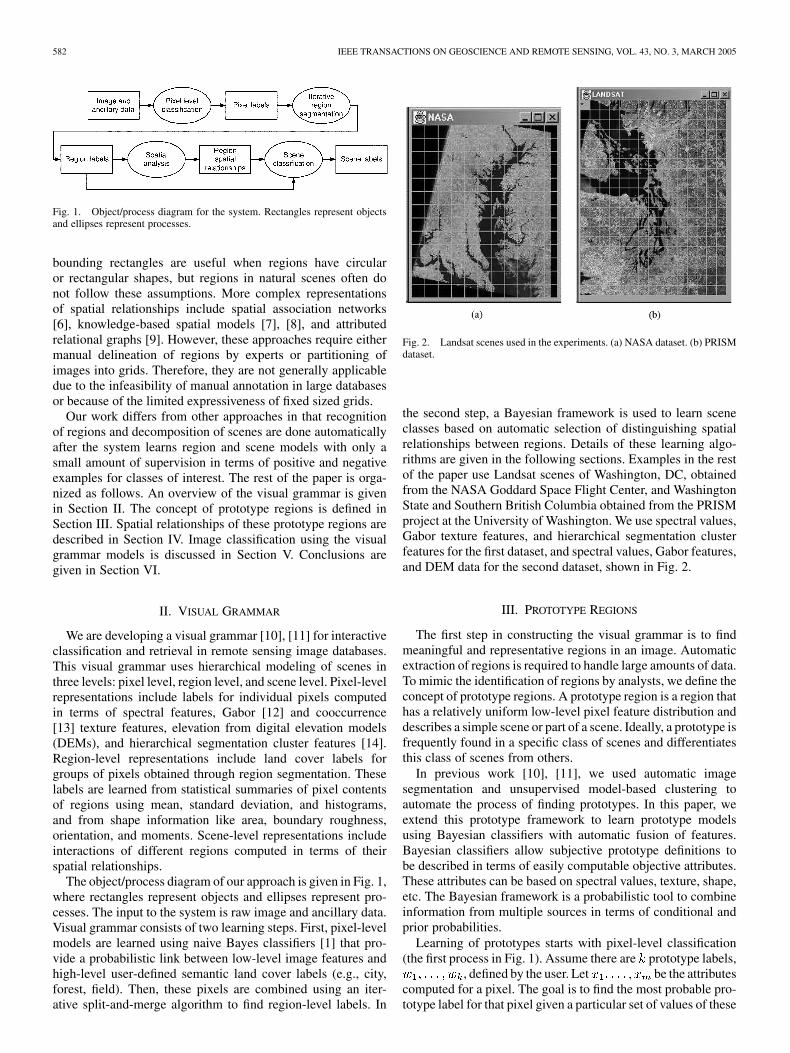
Fig. 2. Landsat scenes used in the experiments. (a) NASA dataset. (b) PRISMdataset.

the second step, a Bayesian framework is used to learn sceneclasses based on automatic selection of distinguishing spatialrelationships between regions. Details of these learning algo-rithms are given in the following sections. Examples in the restof the paper use Landsat scenes of Washington, DC, obtainedfrom the NASA Goddard Space Flight Center, and WashingtonState and Southern British Columbia obtained from the PRISMproject at the University of Washington. We use spectral values,Gabor texture features, and hierarchical segmentation clusterfeatures for the first dataset, and spectral values, Gabor features,and DEM data for the second dataset, shown in Fig. 2.

III. PROTOTYPE REGIONS

The first step in constructing the visual grammar is to findmeaningful and representative regions in an image. Automaticextraction of regions is required to handle large amounts of data.To mimic the identification of regions by analysts, we define theconcept of prototype regions. A prototype region is a region thathas a relatively uniform low-level pixel feature distribution anddescribes a simple scene or part of a scene. Ideally, a prototype isfrequently found in a specific class of scenes and differentiatesthis class of scenes from others.

In previous work [10], [11], we used automatic imagesegmentation and unsupervised model-based clustering toautomate the process of finding prototypes. In this paper, weextend this prototype framework to learn prototype modelsusing Bayesian classifiers with automatic fusion of features.Bayesian classifiers allow subjective prototype definitions tobe described in terms of easily computable objective attributes.These attributes can be based on spectral values, texture, shape,etc. The Bayesian framework is a probabilistic tool to combineinformation from multiple sources in terms of conditional andprior probabilities.

Learning of prototypes starts with pixel-level classification(the first process in Fig. 1). Assume there are prototype labels,

, defined by the user. Let be the attributescomputed for a pixel. The goal is to find the most probable pro-totype label for that pixel given a particular set of values of these

AKSOY et al.: LEARNING BAYESIAN CLASSIFIERS FOR SCENE CLASSIFICATION WITH A VISUAL GRAMMAR 583

attributes. The degree of association between the pixel and pro-totype can be computed using the posterior probability

(1)

under the conditional independence assumption. The condi-tional independence assumption simplifies learning because theparameters for each attribute model can be estimatedseparately. Therefore, user interaction is only required for thelabeling of pixels as positive or negative examplesfor a particular prototype label under training. Models for dif-ferent prototypes are learned separately from the correspondingpositive and negative examples. Then, the predicted prototypebecomes the one with the largest posterior probability and thepixel is assigned the prototype label

(2)

We use discrete variables in the Bayesian model where con-tinuous features are converted to discrete attribute values usingan unsupervised clustering stage based on the -means algo-rithm. The number of clusters is empirically chosen for eachfeature. Clustering is used for processing continuous features(spectral, Gabor, and DEM) and discrete features (hierarchicalsegmentation clusters) with the same tools. (An alternative isto use a parametric distribution assumption, e.g., Gaussian,for each individual continuous feature, but these parametricassumptions do not always hold.) In the following, we describelearning of the models for using the positive trainingexamples for the th prototype label. Learning ofis done the same way using the negative examples.

For a particular prototype, let each discrete variable havepossible values (states) with probabilities

(3)

where , and is the set of param-eters for the th attribute model. This corresponds to a multino-mial distribution. Since maximum-likelihood estimates can giveunreliable results when the sample is small and the number ofparameters is large, we use the Bayes estimate of that can becomputed as the expected value of the posterior distribution.

We can choose any prior for in the computation of the pos-terior distribution, but there is a big advantage to use conjugatepriors. A conjugate prior is one which, when multiplied with thedirect probability, gives a posterior probability having the samefunctional form as the prior, thus allowing the posterior to beused as a prior in further computations [15]. The conjugate priorfor the multinomial distribution is the Dirichlet distribution [16].Geiger and Heckerman [17] showed that if all allowed states ofthe variables are possible (i.e., ) and if certain parameterindependence assumptions hold, then a Dirichlet distribution isindeed the only possible choice for the prior.

Given the Dirichlet priorwhere are positive constants, the posterior distribution of

can be computed using the Bayes rule as

(4)

where is the training sample, and is the number of casesin in which . Then, the Bayes estimate for can befound by computing the conditional expected value

(5)

where and .An intuitive choice for the hyperparameters of

the Dirichlet distribution is the Laplace’s uniform prior [18] thatassumes all states to be equally probable

which results in the Bayes estimate

(6)

Laplace’s prior was decided to be a safe choice when the dis-tribution of the source is unknown and the number of possiblestates is fixed and known [19].

Given the current state of the classifier that was trained usingthe prior information and the sample , we can easily updatethe parameters when new data is available. The new posteriordistribution for becomes

(7)

With the Dirichlet priors and the posterior distribution forgiven in (4), the updated posterior distribution be-

comes

(8)

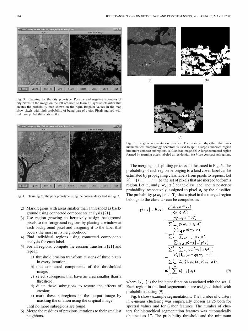
where is the number of cases in in which . Hence,updating the classifier parameters involves only updating thecounts in the estimates for . Figs. 3 and 4 illustrate learningof prototype models from positive and negative examples.

The Bayesian classifiers that are learned as above are used tocompute probability maps for all semantic prototype labels andassign each pixel to one of the labels using the maximum a pos-teriori probability (MAP) rule. In previous work [20], we used aregion merging algorithm to convert these pixel-level classifica-tion results to contiguous region representations. However, wealso observed that this process often resulted in large connectedregions and these large regions with very fractal shapes may notbe very suitable for spatial relationship computations.

We improved the segmentation algorithm (the second processin Fig. 1) using mathematical morphology operators [21] to au-tomatically divide large regions into more compact subregions.Given the probability maps for all labels where each pixel is as-signed either to one of the labels or to the reject class for proba-bilities smaller than a threshold (latter type of pixels are initiallymarked as background), the segmentation process proceeds asfollows.

1) Merge pixels with identical labels to find the initial set ofregions and mark these regions as foreground.


Fig. 3. Training for the city prototype. Positive and negative examples ofcity pixels in the image on the left are used to learn a Bayesian classifier thatcreates the probability map shown on the right. Brighter values in the mapshow pixels with high probability of being part of a city. Pixels marked withred have probabilities above 0.9.

Fig. 4. Training for the park prototype using the process described in Fig. 3.

2) Mark regions with areas smaller than a threshold as back-ground using connected components analysis [21].

3) Use region growing to iteratively assign backgroundpixels to the foreground regions by placing a window ateach background pixel and assigning it to the label thatoccurs the most in its neighborhood.

4) Find individual regions using connected componentsanalysis for each label.

5) For all regions, compute the erosion transform [21] andrepeat:

a) threshold erosion transform at steps of three pixelsin every iteration;

b) find connected components of the thresholdedimage;

c) select subregions that have an area smaller than athreshold;

d) dilate these subregions to restore the effects oferosion;

e) mark these subregions in the output image bymasking the dilation using the original image;

until no more subregions are found.6) Merge the residues of previous iterations to their smallest

neighbors.

(a) (b)

(c)

Fig. 5. Region segmentation process. The iterative algorithm that usesmathematical morphology operators is used to split a large connected regioninto more compact subregions. (a) Landsat image, (b) A large connected regionformed by merging pixels labeled as residential, (c) More compact subregions.

The merging and splitting process is illustrated in Fig. 5. Theprobability of each region belonging to a land cover label can beestimated by propagating class labels from pixels to regions. Let

be the set of pixels that are merged to form aregion. Let and be the class label and its posteriorprobability, respectively, assigned to pixel by the classifier.The probability that a pixel in the merged regionbelongs to the class can be computed as

(9)

where is the indicator function associated with the set .Each region in the final segmentation are assigned labels withprobabilities using (9).

Fig. 6 shows example segmentations. The number of clustersin -means clustering was empirically chosen as 25 both forspectral values and for Gabor features. The number of clus-ters for hierarchical segmentation features was automaticallyobtained as 17. The probability threshold and the minimum


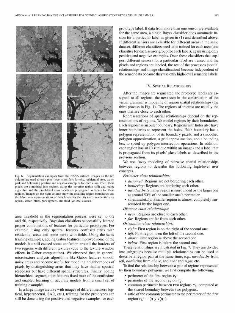
Fig. 6. Segmentation examples from the NASA dataset. Images on the leftcolumn are used to train pixel-level classifiers for city, residential area, water,park and field using positive and negative examples for each class. Then, thesepixels are combined into regions using the iterative region split-and-mergealgorithm and the pixel-level class labels are propagated as labels for theseregions. Images on the right column show the resulting region boundaries andthe false color representations of their labels for the city (red), residential area(cyan), water (blue), park (green), and field (yellow) classes.

area threshold in the segmentation process were set to 0.2and 50, respectively. Bayesian classifiers successfully learnedproper combinations of features for particular prototypes. Forexample, using only spectral features confused cities withresidential areas and some parks with fields. Using the sametraining examples, adding Gabor features improved some of themodels but still caused some confusion around the borders oftwo regions with different textures (due to the texture windoweffects in Gabor computation). We observed that, in general,microtexture analysis algorithms like Gabor features smoothnoisy areas and become useful for modeling neighborhoods ofpixels by distinguishing areas that may have similar spectralresponses but have different spatial structures. Finally, addinghierarchical segmentation features fixed most of the confusionsand enabled learning of accurate models from a small set oftraining examples.

In a large image archive with images of different sensors (op-tical, hyperspectral, SAR, etc.), training for the prototypes canstill be done using the positive and negative examples for each

prototype label. If data from more than one sensor are availablefor the same area, a single Bayes classifier does automatic fu-sion for a particular label as given in (1) and described above.If different sensors are available for different areas in the samedataset, different classifiers need to be trained for each area (oneclassifier for each sensor group for each label), again using onlypositive and negative examples. Once these classifiers that sup-port different sensors for a particular label are trained and thepixels and regions are labeled, the rest of the processes (spatialrelationships and image classification) become independent ofthe sensor data because they use only high-level semantic labels.

IV. SPATIAL RELATIONSHIPS

After the images are segmented and prototype labels are as-signed to all regions, the next step in the construction of thevisual grammar is modeling of region spatial relationships (thethird process in Fig. 1). The regions of interest are usually theones that are close to each other.

Representations of spatial relationships depend on the rep-resentations of regions. We model regions by their boundaries.Each region has an outer boundary. Regions with holes also haveinner boundaries to represent the holes. Each boundary has apolygon representation of its boundary pixels, and a smoothedpolygon approximation, a grid approximation, and a boundingbox to speed up polygon intersection operations. In addition,each region has an ID (unique within an image) and a label thatis propagated from its pixels’ class labels as described in theprevious section.

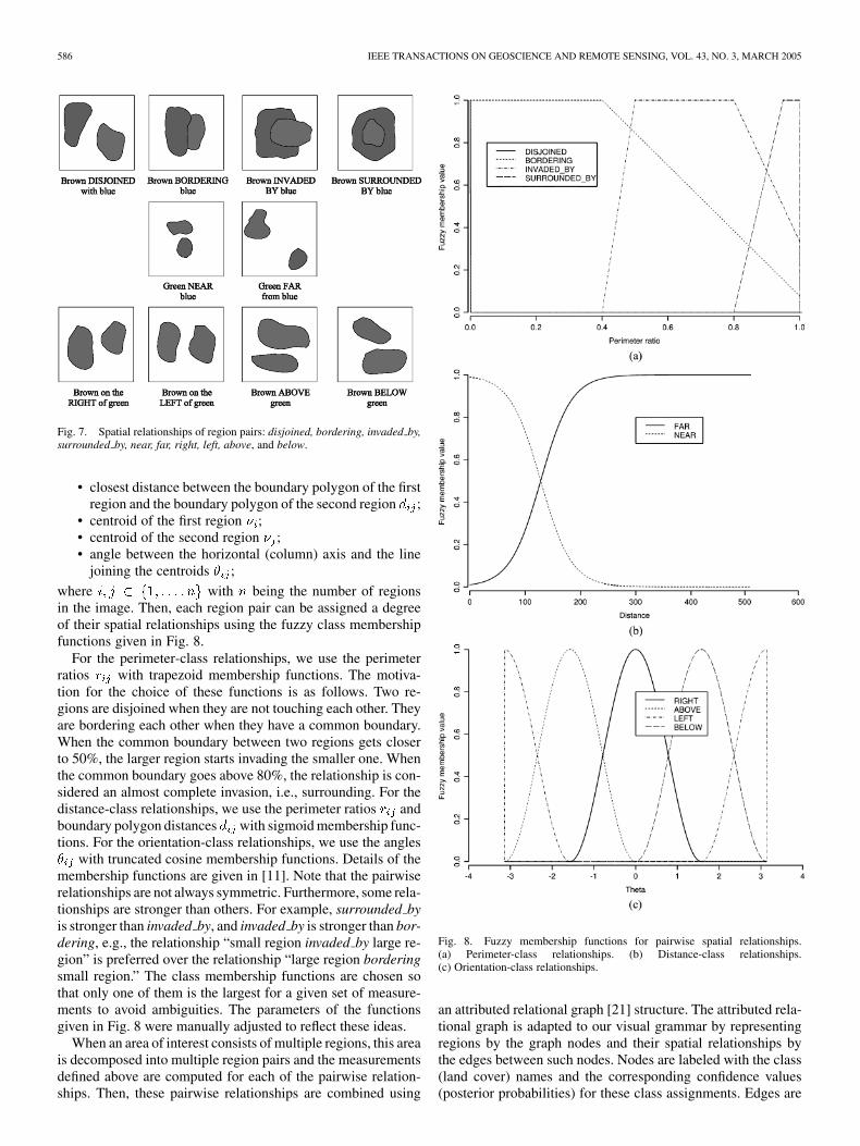
We use fuzzy modeling of pairwise spatial relationshipsbetween regions to describe the following high-level userconcepts.

Perimeter-class relationships:

• disjoined: Regions are not bordering each other.• bordering: Regions are bordering each other.• invaded by: Smaller region is surrounded by the larger one

at around 50% of the smaller one’s perimeter.• surrounded by: Smaller region is almost completely sur-

rounded by the larger one.Distance-class relationships:

• near: Regions are close to each other.• far: Regions are far from each other.

Orientation-class relationships:

• right: First region is on the right of the second one.• left: First region is on the left of the second one.• above: First region is above the second one.• below: First region is below the second one.

These relationships are illustrated in Fig. 7. They are dividedinto subgroups because multiple relationships can be used todescribe a region pair at the same time, e.g., invaded by fromleft, bordering from above, and near and right, etc.

To find the relationship between a pair of regions representedby their boundary polygons, we first compute the following:

• perimeter of the first region ;• perimeter of the second region ;• common perimeter between two regions computed as

the shared boundary between two polygons;• ratio of the common perimeter to the perimeter of the first

region ;


Fig. 7. Spatial relationships of region pairs: disjoined, bordering, invaded by,surrounded by, near, far, right, left, above, and below.

• closest distance between the boundary polygon of the firstregion and the boundary polygon of the second region ;

• centroid of the first region ;• centroid of the second region ;• angle between the horizontal (column) axis and the line

joining the centroids ;

where with being the number of regionsin the image. Then, each region pair can be assigned a degreeof their spatial relationships using the fuzzy class membershipfunctions given in Fig. 8.

For the perimeter-class relationships, we use the perimeterratios with trapezoid membership functions. The motiva-tion for the choice of these functions is as follows. Two re-gions are disjoined when they are not touching each other. Theyare bordering each other when they have a common boundary.When the common boundary between two regions gets closerto 50%, the larger region starts invading the smaller one. Whenthe common boundary goes above 80%, the relationship is con-sidered an almost complete invasion, i.e., surrounding. For thedistance-class relationships, we use the perimeter ratios andboundary polygon distances with sigmoid membership func-tions. For the orientation-class relationships, we use the angles

with truncated cosine membership functions. Details of themembership functions are given in [11]. Note that the pairwiserelationships are not always symmetric. Furthermore, some rela-tionships are stronger than others. For example, surrounded byis stronger than invaded by, and invaded by is stronger than bor-dering, e.g., the relationship “small region invaded by large re-gion” is preferred over the relationship “large region borderingsmall region.” The class membership functions are chosen sothat only one of them is the largest for a given set of measure-ments to avoid ambiguities. The parameters of the functionsgiven in Fig. 8 were manually adjusted to reflect these ideas.

When an area of interest consists of multiple regions, this areais decomposed into multiple region pairs and the measurementsdefined above are computed for each of the pairwise relation-ships. Then, these pairwise relationships are combined using

Fig. 8. Fuzzy membership functions for pairwise spatial relationships.(a) Perimeter-class relationships. (b) Distance-class relationships.(c) Orientation-class relationships.

an attributed relational graph [21] structure. The attributed rela-tional graph is adapted to our visual grammar by representingregions by the graph nodes and their spatial relationships bythe edges between such nodes. Nodes are labeled with the class(land cover) names and the corresponding confidence values(posterior probabilities) for these class assignments. Edges are


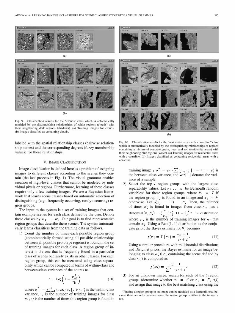
Fig. 9. Classification results for the “clouds” class which is automaticallymodeled by the distinguishing relationships of white regions (clouds) withtheir neighboring dark regions (shadows). (a) Training images for clouds.(b) Images classified as containing clouds.

labeled with the spatial relationship classes (pairwise relation-ship names) and the corresponding degrees (fuzzy membershipvalues) for these relationships.

V. IMAGE CLASSIFICATION

Image classification is defined here as a problem of assigningimages to different classes according to the scenes they con-tain (the last process in Fig. 1). The visual grammar enablescreation of high-level classes that cannot be modeled by indi-vidual pixels or regions. Furthermore, learning of these classesrequire only a few training images. We use a Bayesian frame-work that learns scene classes based on automatic selection ofdistinguishing (e.g., frequently occurring, rarely occurring) re-gion groups.

The input to the system is a set of training images that con-tain example scenes for each class defined by the user. Denotethese classes by . Our goal is to find representativeregion groups that describe these scenes. The system automati-cally learns classifiers from the training data as follows.

1) Count the number of times each possible region group(combinatorially formed using all possible relationshipsbetween all possible prototype regions) is found in the setof training images for each class. A region group of in-terest is the one that is frequently found in a particularclass of scenes but rarely exists in other classes. For eachregion group, this can be measured using class separa-bility which can be computed in terms of within-class andbetween-class variances of the counts as

(10)

where is the within-classvariance, is the number of training images for class

is the number of times this region group is found in

Fig. 10. Classification results for the “residential areas with a coastline” classwhich is automatically modeled by the distinguishing relationships of regionscontaining a mixture of concrete, grass, trees, and soil (residential areas) withtheir neighboring blue regions (water). (a) Training images for residential areaswith a coastline. (b) Images classified as containing residential areas with acoastline.

training image isthe between-class variance, and denotes the vari-ance of a sample.

2) Select the top region groups with the largest classseparability values. Let be Bernoulli randomvariables1 for these region groups, where ifthe region group is found in an image andotherwise. Let . Then, the numberof times is found in images from class has a

Binomial distribution

where is the number of training images for thatcontain . Using a Beta(1, 1) distribution as the conju-gate prior, the Bayes estimate for becomes

(11)

Using a similar procedure with multinomial distributionsand Dirichlet priors, the Bayes estimate for an image be-longing to class (i.e., containing the scene defined byclass ) is computed as

(12)

3) For an unknown image, search for each of the regiongroups (determine whether or )and assign that image to the best matching class using the

1Finding a region group in an image can be modeled as a Bernoulli trial be-cause there are only two outcomes: the region group is either in the image ornot.


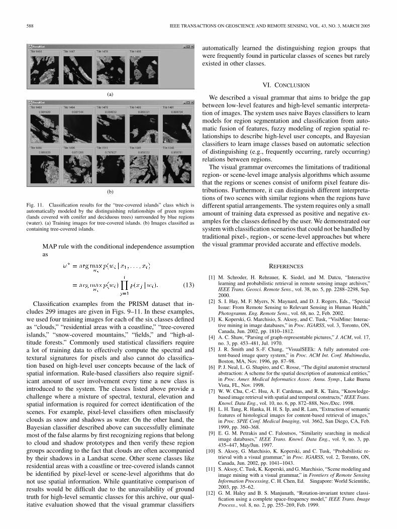
Fig. 11. Classification results for the “tree-covered islands” class which isautomatically modeled by the distinguishing relationships of green regions(lands covered with conifer and deciduous trees) surrounded by blue regions(water). (a) Training images for tree-covered islands. (b) Images classified ascontaining tree-covered islands.

MAP rule with the conditional independence assumptionas

(13)

Classification examples from the PRISM dataset that in-cludes 299 images are given in Figs. 9–11. In these examples,we used four training images for each of the six classes definedas “clouds,” “residential areas with a coastline,” “tree-coveredislands,” “snow-covered mountains,” “fields,” and “high-al-titude forests.” Commonly used statistical classifiers requirea lot of training data to effectively compute the spectral andtextural signatures for pixels and also cannot do classifica-tion based on high-level user concepts because of the lack ofspatial information. Rule-based classifiers also require signif-icant amount of user involvement every time a new class isintroduced to the system. The classes listed above provide achallenge where a mixture of spectral, textural, elevation andspatial information is required for correct identification of thescenes. For example, pixel-level classifiers often misclassifyclouds as snow and shadows as water. On the other hand, theBayesian classifier described above can successfully eliminatemost of the false alarms by first recognizing regions that belongto cloud and shadow prototypes and then verify these regiongroups according to the fact that clouds are often accompaniedby their shadows in a Landsat scene. Other scene classes likeresidential areas with a coastline or tree-covered islands cannotbe identified by pixel-level or scene-level algorithms that donot use spatial information. While quantitative comparison ofresults would be difficult due to the unavailability of groundtruth for high-level semantic classes for this archive, our qual-itative evaluation showed that the visual grammar classifiers

automatically learned the distinguishing region groups thatwere frequently found in particular classes of scenes but rarelyexisted in other classes.

VI. CONCLUSION

We described a visual grammar that aims to bridge the gapbetween low-level features and high-level semantic interpreta-tion of images. The system uses naive Bayes classifiers to learnmodels for region segmentation and classification from auto-matic fusion of features, fuzzy modeling of region spatial re-lationships to describe high-level user concepts, and Bayesianclassifiers to learn image classes based on automatic selectionof distinguishing (e.g., frequently occurring, rarely occurring)relations between regions.

The visual grammar overcomes the limitations of traditionalregion- or scene-level image analysis algorithms which assumethat the regions or scenes consist of uniform pixel feature dis-tributions. Furthermore, it can distinguish different interpreta-tions of two scenes with similar regions when the regions havedifferent spatial arrangements. The system requires only a smallamount of training data expressed as positive and negative ex-amples for the classes defined by the user. We demonstrated oursystem with classification scenarios that could not be handled bytraditional pixel-, region-, or scene-level approaches but wherethe visual grammar provided accurate and effective models.

REFERENCES

[1] M. Schroder, H. Rehrauer, K. Siedel, and M. Datcu, “Interactivelearning and probabilistic retrieval in remote sensing image archives,”IEEE Trans. Geosci. Remote Sens., vol. 38, no. 5, pp. 2288–2298, Sep.2000.

[2] S. I. Hay, M. F. Myers, N. Maynard, and D. J. Rogers, Eds., “SpecialIssue: From Remote Sensing to Relevant Sensing in Human Health,”Photogramm. Eng. Remote Sens., vol. 68, no. 2, Feb. 2002.

[3] K. Koperski, G. Marchisio, S. Aksoy, and C. Tusk, “VisiMine: Interac-tive mining in image databases,” in Proc. IGARSS, vol. 3, Toronto, ON,Canada, Jun. 2002, pp. 1810–1812.

[4] A. C. Shaw, “Parsing of graph-representable pictures,” J. ACM, vol. 17,no. 3, pp. 453–481, Jul. 1970.

[5] J. R. Smith and S.-F. Chang, “VisualSEEk: A fully automated con-tent-based image query system,” in Proc. ACM Int. Conf. Multimedia,Boston, MA, Nov. 1996, pp. 87–98.

[6] P. J. Neal, L. G. Shapiro, and C. Rosse, “The digital anatomist structuralabstraction: A scheme for the spatial description of anatomical entities,”in Proc. Amer. Medical Informatics Assoc. Annu. Symp., Lake BuenaVista, FL, Nov. 1998.

[7] W. W. Chu, C.-C. Hsu, A. F. Cardenas, and R. K. Taira, “Knowledge-based image retrieval with spatial and temporal constructs,” IEEE Trans.Knowl. Data Eng., vol. 10, no. 6, pp. 872–888, Nov./Dec. 1998.

[8] L. H. Tang, R. Hanka, H. H. S. Ip, and R. Lam, “Extraction of semanticfeatures of histological images for content-based retrieval of images,”in Proc. SPIE Conf. Medical Imaging, vol. 3662, San Diego, CA, Feb.1999, pp. 360–368.

[9] E. G. M. Petrakis and C. Faloutsos, “Similarity searching in medicalimage databases,” IEEE Trans. Knowl. Data Eng., vol. 9, no. 3, pp.435–447, May/Jun. 1997.

[10] S. Aksoy, G. Marchisio, K. Koperski, and C. Tusk, “Probabilistic re-trieval with a visual grammar,” in Proc. IGARSS, vol. 2, Toronto, ON,Canada, Jun. 2002, pp. 1041–1043.

[11] S. Aksoy, C. Tusk, K. Koperski, and G. Marchisio, “Scene modeling andimage mining with a visual grammar,” in Frontiers of Remote SensingInformation Processing, C. H. Chen, Ed. Singapore: World Scientific,2003, pp. 35–62.

[12] G. M. Haley and B. S. Manjunath, “Rotation-invariant texture classi-fication using a complete space-frequency model,” IEEE Trans. ImageProcess., vol. 8, no. 2, pp. 255–269, Feb. 1999.


[13] R. M. Haralick, K. Shanmugam, and I. Dinstein, “Textural features forimage classification,” IEEE Trans. Syst., Man, Cybern., vol. SMC-3, no.6, pp. 610–621, Nov. 1973.

[14] J. C. Tilton, G. Marchisio, K. Koperski, and M. Datcu, “Image informa-tion mining utilizing hierarchical segmentation,” in Proc. IGARSS, vol.2, Toronto, ON, Canada, Jun. 2002, pp. 1029–1031.

[15] C. M. Bishop, Neural Networks for Pattern Recognition. Oxford,U.K.: Oxford Univ. Press, 1995.

[16] M. H. DeGroot, Optimal Statistical Decisions. New York: McGraw-Hill, 1970.

[17] D. Geiger and D. Heckerman, “A characterization of the Dirichlet dis-tribution through global and local parameter independence,” Ann. Stat.,vol. 25, no. 3, pp. 1344–1369, 1997.

[18] T. M. Mitchell, Machine Learning. New York: McGraw-Hill, 1997.[19] R. F. Krichevskiy, “Laplace’s law of succession and universal encoding,”

IEEE Trans. Inf. Theory, vol. 44, no. 1, pp. 296–303, Jan. 1998.[20] S. Aksoy, K. Koperski, C. Tusk, G. Marchisio, and J. C. Tilton,

“Learning Bayesian classifiers for a visual grammar,” in Proc. IEEEGRSS Workshop on Advances in Techniques for Analysis of RemotelySensed Data, Washington, DC, Oct. 2003, pp. 212–218.

[21] R. M. Haralick and L. G. Shapiro, Computer and Robot Vi-sion. Reading, MA: Addison-Wesley, 1992.

Selim Aksoy (S’96–M’01) received the B.S. degreefrom Middle East Technical University, Ankara,Turkey, in 1996, and the M.S. and Ph.D. degreesfrom the University of Washington, Seattle, in 1998and 2001, respectively, all in electrical engineering.

He is currently an Assistant Professor in theDepartment of Computer Engineering, BilkentUniversity, Ankara. Before joining Bilkent, he wasa Research Scientist with Insightful Corporation,Seattle, where he was involved in image under-standing and data-mining research sponsored by

the National Aeronautics and Space Administration, the U.S. Army, and theNational Institutes of Health. From 1996 to 2001, he was a Research Assistantwith the University of Washington where he developed algorithms for con-tent-based image retrieval, statistical pattern recognition, object recognition,graph-theoretic clustering, relevance feedback, and mathematical morphology.During summers of 1998 and 1999, he was a Visiting Researcher with theTampere International Center for Signal Processing collaborating in a con-tent-based multimedia retrieval project. His research interests are in computervision, statistical and structural pattern recognition, machine learning and datamining with applications to remote sensing, medical imaging, and multimediadata analysis.

Dr. Aksoy is a member of the International Association for Pattern Recog-nition (IAPR). He was recently elected the Vice Chair of the IAPR TechnicalCommittee on Remote Sensing for the period 2004–2006.

Krzysztof Koperski (S’88–M’90) received theM.Sc. degree in electrical engineering from WarsawUniversity of Technology, Warsaw, Poland, in 1989,and the Ph.D. degree in computer science fromSimon Fraser University, Burnaby, BC, Canada, in1999. During his graduate work at Simon FraserUniversity, he worked on knowledge discovery inspatial databases and spatial data warehousing.

In 1999, he was a Visiting Researcher with the Uni-versity of L’Aquila, working on spatial data mining inthe presence of uncertain information. Since 1999, he

has been with Insightful Corporation, Seattle, WA. His research interests includespatial and image data mining, information visualization, information retrieval,and text mining. He has been involved in projects concerning remote sensingimage classification, medical image processing, data clustering, and natural lan-guage processing.

Carsten Tusk received the diploma degree incomputer science and engineering from theRhineland-Westphalian Technical University,Aachen, Germany, in 2001.

Since August 2001, he has been working as aResearch Scientist with Insightful Corporation,Seattle, WA. His research interests are in informationretrieval, statistical data analysis, and databasesystems.

Giovanni Marchisio received the B.A.Sc. degree inengineering from the University of British Columbia,Vancouver, BC, Canada, and the Ph.D. degree in geo-physics and planetary physics from the Scripps In-stitution of Oceanography, University of California,San Diego.

He is currently Director of Emerging Productswith Insightful Corporation, Seattle, WA. He hasmore than 15 years experience in commercialsoftware development related to text analysis,computational linguistics, image processing, and

multimedia information retrieval methodologies. At Insightful, he has beena Principal Investigator on R&D government contracts totaling several mil-lions (with the National Aeronautics and Space Administration, the NationalInstitutes of Health, the Defense Advanced Research Projects Agency, andthe Department of Defense). He has articulated novel scientific ideas andsoftware architectures in the areas of artificial intelligence, pattern recognition,Bayesian and multivariate inference, latent semantic analysis, cross-languageretrieval, satellite-image-mining World Wide Web-based environment for videoand image compression and retrieval. He has also been a Senior Consultanton statistical modeling and prediction analysis of very large databases ofmultivariate time series. He has authored and coauthored several articles orbook chapters on multimedia data mining. In the past three years, he hasproduced several inventions for information retrieval and knowledge discovery,which led to three U.S. patents. He also has also been a Visiting Professorwith the University of British Columbia. His previous work includes researchin signal processing, ultrasound acoustic imaging, seismic reflection, andelectromagnetic induction imaging of the earth’s interior.

James C. Tilton (S’79–M’81–SM’94) received theB.A. degrees in electronic engineering, environ-mental science and engineering, and anthropology,the M.E.E. degree in electrical engineering fromRice University, Houston, TX, in 1976, the M.S.degree in optical sciences from the University ofArizona, Tucson, in 1978, and the Ph.D. degree inelectrical engineering from Purdue University, WestLafayette, IN, in 1981.

He is currently a Computer Engineer with the Ap-plied Information Science Branch (AISB), Earth and

Space Data Computing Division, NASA Goddard Space Flight Center, Green-belt, MD. He was previously with the Computer Sciences Corporation, SilverSpring, MD, from 1982 to 1983, and Science Applications Research, Riverdale,MD, from 1983 to 1985 on contracts with NASA Goddard. As a member of theAISB, he is responsible for designing and developing computer software toolsfor space and earth science image analysis algorithms, and encouraging the useof these computer tools through interactions with space and earth scientists. Hisdevelopment of a recursive hierarchical segmentation algorithm has resulted intwo patent applications. He is an Associate Editor for Pattern Recognition.

Dr. Tilton is a member of the IEEE Geoscience and Remote Sensing andSignal Processing Societies and is a member of Phi Beta Kappa, Tau Beta Pi, andSigma Xi. From 1992 through 1996, he served as a member of the IEEE Geo-science and Remote Sensing Society Administrative Committee. Since 1996, hehas served as an Associate Editor for the IEEE TRANSACTIONS ON GEOSCIENCE

AND REMOTE SENSING.

learning bayesian classifiers for scene classification

Documents